Online Stochastic Packing applied to
Display Ad Allocation

Abstract

Inspired by online ad allocation, we study online stochastic packing linear programs from theoretical and practical standpoints. We first present a near-optimal online algorithm for a general class of packing linear programs which model various online resource allocation problems including online variants of routing, ad allocations, generalized assignment, and combinatorial auctions. As our main theoretical result, we prove that a simple primal-dual training-based algorithm achieves a $(1-o(1))$-approximation guarantee in the random order stochastic model. This is a significant improvement over logarithmic or constant-factor approximations for the adversarial variants of the same problems (e.g. factor $1-{1\over e}$ for online ad allocation, and $\log(m)$ for online routing). We then focus on the online display ad allocation problem and study the efficiency and fairness of various training-based and online allocation algorithms on data sets collected from real-life display ad allocation system. Our experimental evaluation confirms the effectiveness of training-based primal-dual algorithms on real data sets, and also indicate an intrinsic trade-off between fairness and efficiency.

1 Introduction

Online stochastic optimization is a central problem in operations research with many applications in dynamic resource allocation. In these settings, given a set of resources, demands for the resources arrive online, with associated values; given a general prior about the demands, one has to decide whether and how to satisfy (i.e., allocate the desired resources to) a demand when it arrives. The goal is to find a valid assignment with maximum total value. Such problems appear in many areas including online routing [13, 4], online combinatorial auctions [16], online ad allocation problems [32, 18, 19], and online dynamic pricing and inventory management problems. For example, in routing problems, we are given a network with capacity constraints over edges; customers arrive online and bid for a subset of edges (typically a path) in the network, and the goal is to assign paths to new customers so as to maximize the total social welfare. Similarly, in online combinatorial auctions, bidders arrive online and may bid on a subset of resources; the auctioneer should decide whether to sell those resources to the bidder. In the display ads problem, when users visit a website, the website publisher has to choose ads to show them so as to maximize the value of the displayed ads. In this paper, we study these online stochastic resource allocation problems from theoretical and practical standpoints. Our theoretical results apply to a general set of problems including all those discussed above. Our practical results apply to the problem of display ads and give additional validation of our theoretical models and results.

More specifically, we consider the following general class of packing linear programs (PLP): Let $J$ be a set of $m$ resources; each resource $j\in J$ has a capacity $c_{j}$. The set of resources and their capacities are known in advance. Let $I$ be a set of $n$ agents that arrive one by one online, each with a set of options $O_{i}$. Each option $o\in O_{i}$ of agent $i$ has an associated value $w_{io}\geq 0$ and requires $a_{ioj}\geq 0$ units of each resource $j$. The set of options and the values $w_{io}$ and $a_{ioj}$ arrive together with agent $i$. When an agent arrives, the algorithm has to immediately decide whether to assign the agent and if so, which option to choose. The goal is to find a maximum-value allocation that does not allocate more of any resource than is available.

In the adversarial or worst-case setting, no online algorithm can achieve any non-trivial competitive ratio; consider the simple case of one resource with capacity one and two agents. For each agent there are just two options, namely to get the resource or not to get it. If an agent gets the resource, he uses its whole capacity. The first agent has value 100 for getting the resource and value 0 for not getting the resource. If he is assigned the resource, then the value of the second agent for getting the resource is 10000, otherwise it is 1. In both cases the algorithm achieves less than 1/100th of the value of the optimal solution. This example can easily be generalized to show that no non-trivial competetive ratio is possible.

Since in the adversarial setting the lack of prior information about the arrival rate of different types of agents implies strong impossibility results, it is natural to consider stochastic settings for online allocation problems, where we may have some prior information about the arrival rate of different types of agents. In particular, we consider the random-order stochastic model, where the order in which impressions arrive is random, but we do not have any other prior information. We present a training-based online algorithm for the general class of packing linear programs described above and prove that in the random-order stochastic model, it achieves an approximation ratio of $1-\varepsilon$ under some mild assumptions. This result also implies the same result in the i.i.d. model.

Our training-based primal-dual algorithm for the stochastic PLP problem observes the first $\varepsilon$ fraction of the input and then solves an LP on this instance. (This requires knowing the number of agents in advance, which is unavoidable for any sub-logarithmic approximation; see Theorem 9.) For each resource, the corresponding dual variable extracted from this LP serves as a (posted) price per unit of the resource for the remaining agents. The algorithm allocates to each remaining agent the option maximizing his utility, defined as the difference between the value of an option and the price he must pay to obtain the necessary resources. We prove that this algorithm provides a $1-\varepsilon$ approximation for the large class of natural packing problems we consider, provided that no individual option for any agent consumes too much of any resource or provides too large a fraction of the total value. Specifically we show the following result. Recall that $n$ and $m$ denote the number of agents and resources respectively; $q$ denotes $\max_{i}|O_{i}|$ and OPT the value of an optimal off-line solution to the PLP problem.

Theorem 1.

The Training-Based Primal-Dual algorithm is $(1-O(\varepsilon))$-competitive (a PTAS) for the online stochastic PLP problem with high probability, as long as (1) $\max_{i,o}\left\{\frac{w_{io}}{\textsc{OPT}}\right\}\leq\frac{\varepsilon}{(m+1)(\ln n+\ln q)}$ and (2) $\max_{i,o,j}\left\{\frac{a_{ioj}}{c_{j}}\right\}\leq\frac{\varepsilon^{3}}{(m+1)(\ln n+\ln q)}$.

1.1 Applications

Theorem 1 has many applications; we elaborate on several, including routing problems, online combinatorial auctions, the display ad problem, and the adword allocation problem. For each of these problems, we improve on the known results for the online version. In each, we will comment on the interpretation of the two conditions of Theorem 1 in that application.

In the online routing problem, we are initially given a network with capacity constraints over the $m$ edges. When a customer $i\in I$ arrives online, she wishes to send $d_{i}$ units of flow between some vertices $s_{i}$ and $t_{i}$, and derives $w_{i}$ units of value from sending such flow. Thus, the set of options $O_{i}$ for customer $i$ is the set of all $s_{i}-t_{i}$ paths in the network. The algorithm must pick a set of customers $I^{*}\subseteq I$, and satisfy their demands by allocating a path to each of them while respecting the capacity constraints on each edge; the goal is to maximize the total value of satisfied customers. For this problem, the dual variables learned from the sample yield a price for each edge; each customer is allocated the minimum-cost $s_{i}-t_{i}$ path if its cost is no more than $w_{i}$. In road networks, for instance, these dual variables can be interpreted as the tolls to be charged to prevent congestion. Theorem 1 applies when the contributions of individual agents/vehicles to the total objective or to road congestion are small. As one such example, over a million vehicles enter or leave Manhattan daily, with the George Washington Bridge alone carrying several hundred thousand. Online routing problems have been studied extensively in the adversarial model when demands can be large, and there are (poly)-logarithmic lower and upper bounds even for special cases [4, 13]. Our approach gives a $1-o(1)$-approximation for the described stochastic variants of these problems.

In the combinatorial auction problem, we are initally given a set $J$ of $m$ goods, with $c_{j}$ units for each good $j\in J$. Agents arrive online, and the options for agent $i$ may include different bundles of goods he values differently; option $o\in O_{i}$ provides $w_{io}$ units of value, and requires $a_{ioj}$ units of good $j$. We wish to find a valid allocation maximizing social welfare. Here, the dual variables learned from the sample yield a price per unit of each good; each agent picks the option that maximizes his utility. Here Theorem 1 applies as long as no individual agent controls a large fraction of the market, and as long as the set of options for any single agent is at most exponential in the number of resources. These conditions often hold, as in cases when bidders are single-minded or the number of bundles they are interested in is polynomial in $n$, or if their options correspond to using different subsets of the resources. We also observe that the posted prices result in a take-it-or-leave it auction, and thus a truthful online allocation mechanism. Revenue maximization in online auctions using sequence item pricing has been explored recently in the literature [6, 16]. [16] achieves constant-factor approximations for these problems in more general models than we consider.

In the Display Ads Allocation (DA) problem [19], there is a set $J$ of $m$ advertisers who have paid a web publisher for their ads to be shown to visitors to the website. The contract bought by advertiser $j$ specifies an integer upper bound on the number $n(j)$ of impressions that $j$ is willing to pay for. A set $I$ of impressions arrives online, each impression $i$ with a value $w_{ij}\geq 0$ for advertiser $j$. Each impression can be assigned to at most one advertiser, i.e., there are $m$ options for each impression, and each option $o$ has $a_{ioj}=1$ for advertiser $j$. The goal is to maximize the value of all the assigned impressions. The dual variables learned from the sample yield a discount factor $\beta_{j}$ for each advertiser $j$, and the algorithm is to assign an impression to advertiser $j$ that maximizes $w_{ij}-\beta_{j}$. The contracts for advertisers typically involve thousands of impressions, so the contribution of any one impression/agent is small, and the hypotheses of Theorem 1 hold. The adversarial online DA problem was considered in [19], which showed that the problem was inapproximable without exploiting free disposal; using this property, a simple greedy algorithm is $1\over 2$-competitive, which is optimal. When the demand of each advertiser is large, a $(1-{1\over e})$-competitive algorithm exists (see [19] for details of the model and results), and this is the best possible. For the unweighted (max-cardinality) version of this problem in the i.i.d. model, a $0.67$-competitive algorithm has been recently developed [20]; this improves the known $1-{1\over e}$-approximation algorithm for online stochastic matching [25].

The AdWords (AW) problem [32, 18] is related to the DA problem; here we allocate impressions resulting from search queries. Advertiser $j$ has a budget $b(j)$ instead of a bound $n(j)$ on the number of impressions. Assigning impression $i$ to advertiser $j$ consumes $w_{ij}$ units of $j$’s budget instead of 1 of the $n(j)$ slots, as in the DA problem. Several approximation algorithms have been designed for the offline AW problem [15, 34, 5]. For the online setting, if every weight is very small compared to the corresponding budget, there exist $(1-{1\over e})$-competitive online algorithms [32, 12, 24, 2], and this factor is tight. In order to go beyond the competitive ratio of $1-{1\over e}$ in the adversarial model, stochastic online settings have been studied, such as the random order and i.i.d models [24]. Devanur and Hayes [18] described a primal-dual ($1-\varepsilon$)-approximation algorithm for this problem in the random order model, with the assumption that OPT is larger than $O({m^{2}\over\varepsilon^{3}})$ times each $w_{ij}$, where $m$ is the number of advertisers; Theorem 1 can be viewed as generalizing this result to a much larger class of problems.

1.2 Experimental Validation

For the applications described above, stochastic models are reasonable as the algorithm often has an idea of what agents to expect. For example, in the Display Ad Allocation problem, agents correspond to users visiting the website of a publisher who has sold contracts to advertisers. As the publisher most likely sees similar user traffic patterns from day to day, he has an idea of the available ad inventory based on historical data. In Section 5, we perform preliminary experiments on real instances of the DA problem, using actual display ad data for a set of anonymous publishers. As with any real application, there are additional features of the problem, and in the one we considered, both fairness and efficiency were important metrics. Hence, we also evaluated our algorithms for fairness (see Section 3 for a precise definition); we compared the efficiency and fairness of our training-based algorithm with those of algorithms from [19] designed for the adversarial setting, as well as hybrid algorithms combining the two approaches. We propose a new approach for evaluating the fairness of an allocation, based on finding an “ideal” fair allocation, and measuring the distance to that allocation. Our experimental results validate Theorem 1 for this application, as they show that on this real data set, training indeed helps efficiency by 5-12%, and that the online algorithms from [19] are significantly better than a simple greedy approach.

1.3 Other Related Work

Our proof technique is similar to that of [18] for the AW problem; it is based on their observation that dual variables satisfy the complemtary slackness conditions of the first $\varepsilon$ fraction of impressions and approximately satisfy these conditions on the entire set. However, one key difference is that in the AW problem, the coefficients for variable $x_{ij}$ in the linear program are the same in both the constraint and the objective function. That is, the contribution an impression makes to an advertisers value is identical to the amount of budget it consumes. In contrast, in the general class of packing problems that we study, these coefficients are unrelated, which complicates the proof.

The random-order model has been considered for several problems, often called secretary problems. The elements arriving online are often the ground set of an appropriate matroid, and the goal is to find a maximum weight independent set in the matroids; such problems include finding a maximum value set of $k$ elements [27], or finding a maximum spanning forest in a graph when edges appear online. Other secretary problems include finding a maximum weight set of items that fits in a Knapsack. (See [6] for a survey of these and other results.) Constant-competitive algorithms are known for these problems; without additional assumptions (such as those of Theorem 1), no algorithm can achieve a competitive ratio better than $1/e$. Specifically for the DA problem, the results of [28] imply that the random-order model permits a $1/8$-competitive algorithm even without using the free disposal property or the conditions of Theorem 1.

There have been recent results regarding ad allocation strategies in display advertising in hybrid settings with both contract-based advertisers and spot market advertisers  [22, 21]. Our results in this paper may be interpreted as a class of representative bidding strategies that can be used on behalf of contract-based advertisers competing with the spot market bidders [22]. There are many other interesting problems in ad serving systems related to information retrieval and data mining [9, 11, 10] as well as various optimal caching strategies [33, 17]; our focus in this paper is on online allocation problems.]

It was recently brought to our attention that subsequent to the submission of an earlier version of this paper (including our main result), similar results (obtained independently) were posted in a working paper[1].

2 A Training-based PTAS

In this section, we present the primal-dual training-based algorithm for the online stochastic packing problem, and prove Theorem 1: That is, under mild (practically-motivated) assumptions, the algorithm achieves an approximation factor of $1-\varepsilon$.

Our algorithm examines the first $\varepsilon n$ agents in order before solving a Linear Program to compute the posted prices used for the remaining agents. This requires advance knowledge of the number of agents that will arrive; Theorem 9 at the end of this section shows that this is unavoidable. Recall that there is a set $I$ of “agents”; agent $i\in I$ has a set of mutually exclusive options $O_{i}$, and we use an indicator variable $x_{io}$ to denote whether agent $i$ selects alternative $o\in O_{i}$. Each option for an agent may have a different “size” in each constraint; we use $a_{ioj}$ to denote the size in constraint $j$ of option $o$ for agent $i$. We use $w_{io}$ to denote the value from selecting option $o$ for agent $i$, and $c_{j}$ is the “capacity” of constraint $j$. That is, our goal is to maximize $w^{T}x$ while picking at most one option for each agent, and subject to $Ax\leq c$. Subsequently, we normalize $A,c$ such that $c$ is the all-1’s vector, and write the (normalized) primal linear program below. We also use the dual linear program, which introduces a variable $\beta_{j}$ for each constraint $j$.

Primal-LP

$$\max\sum_{i}\sum_{o\in O_{i}}w_{io}x_{io}$$

$$\sum_{o\in O_{i}}x_{io}\ \leq \quad 1 (\forall\ i)$$

$$\sum_{i,o}a_{ioj}x_{io}\ \leq \quad 1 (\forall\ j)$$

$$x_{io}\ \geq \quad 0 (\forall\ i,o)$$

Dual-LP

$$\min\sum_{j}\beta_{j}\ + \sum_{i}z_{i}$$

$$z_{i}+\sum_{j}\beta_{j}a_{ioj}\ \geq \quad w_{io} (\forall i,o)$$

$$\beta_{j},z_{i}\ \geq \quad 0 (\forall i,j)$$

Let $n$ be the total number of agents, $q=\max_{i}|O_{i}|$ be the maximum number of options for any agent, and $m$ be the number of constraints. We say that the gain from option $o\in O_{i}$ is $w_{io}-\sum_{j}\beta^{*}_{j}a_{ioj}$. The Training-Based Primal-Dual Algorithm proceeds as follows:

1. Let $S$ denote the first $\varepsilon n$ agents in the sequence. For the purposes purposes of analysis, these agents are not selected. (Our implementations may assign these impressions according to some online algorithm.)

2. Solve the Dual-LP on the agents in $S$, with the objective function containing the term $\varepsilon\beta_{j}$ instead of $\beta_{j}$ for each $j\in[m]$. (This is equivalent to reducing the capacity of a constraint from 1 to $\varepsilon$; we refer to this as a reduced instance.) Let $\beta^{*}_{j}$ denote the value of the dual variable for constraint $j$ in this optimal solution.

3. For each subsequent agent $i$, if there is an option $o$ with non-negative gain, select the option $o$ of maximum gain, and set $z_{i}=\textit{gain}(o)$.

We will refer to a variant of this algorithm in Section 5 as the $\mathsf{DualBase}$ algorithm. The intuition behind this algorithm is simple; the dual variables $\beta^{*}_{j}$ can be thought of as specifying a value/size ratio necessary for an option to be selected. An optimal choice for each $\beta_{j}$ gives an optimal solution to the packing problem; this fact is proven implicitly in the next section, where we further show that with high probability, the optimal choice $\beta^{*}_{j}$ on the sample $S$ leads to a near-optimal solution on the entire instance. In the following, let $w_{\max}=\max_{i,o}\{w_{io}\}$, and let $a_{\max}=\max_{i,o,j}\{a_{ioj}\}$.

2.1 Proof of Theorem 1

We now prove Theorem 1, showing that the above training-based algorithm is a polynomial-time approximation scheme. ( Proofs of some claims are in Appendix LABEL:app:proofs.) Let $I^{*}\subseteq I$ denote the set of agents $i$ with some option $o$ having non-negative gain, and let $\mathcal{O}^{*}$ denote the set of pairs $\{(i,o)\mid i\in I^{*},o=\arg\max_{o\in O(i)}\textit{gain}(o)\}$. We abuse notation by writing $i\in\mathcal{O}^{*}$ if there exists $o\in O(i)$ such that $(i,o)\in\mathcal{O}^{*}$. We use $\mathcal{O}^{*}(S)$ to denote $\mathcal{O}^{*}\cap S$; note that $\mathcal{O}^{*}-\mathcal{O}^{*}(S)$ represents the options selected by the algorithm (for the purposes of analysis, we do not select any options for agents in $S$).

Given a vector $\beta^{*}$, we obtain a feasible solution to Dual-LP by selecting for each item in $I^{*}$, the option $o$ such that $(i,o)\in\mathcal{O}^{*}$ and setting $z_{i}=\textit{gain}(o)$.

Definition 2.

Let $W=\sum_{(i,o)\in\mathcal{O}^{*}}w_{io}$ be the total weight of selected options, and let $W(S)=\sum_{(i,o)\in\mathcal{O}^{*}(S)}w_{io}$. Let $C(j)=\sum_{(i,o)\in\mathcal{O}^{*}}a_{ioj}$ and $C(j,S)=\sum_{(i,o)\in\mathcal{O}^{*}(S)}a_{ioj}$.

For any fixed vector $\beta^{*}$, $\mathcal{O}^{*}$ and hence $W$ and each $C(j)$ are independent of the choice of the sample $S$; the expected value of $W(S)$ is $\varepsilon W$, and that of $C(j,S)$ is $\varepsilon C(j)$. The main idea of the proof is that if $\beta^{*}$ satisfies the complentary slackness conditions on the first $\varepsilon n$ impressions (being an optimal solution), w.h.p. it approximately satisfies these conditions on the entire set. Thus, we conclude that the values of $W(S)$ and $C(j,S)$ are likely to be close to their expectations.

The following lemma proved by [18], an application of the Chernoff-Hoeffding bounds, is of use:

Lemma 3 ([18]).

Let $Y=\{Y_{1},\ldots,Y_{n}\}$ be a set of real numbers, and let $0<\varepsilon<1$. Let $S$ be a random subset of $Y$ of size $\varepsilon n$ and let $Y_{S}=\sum_{i\in S}Y_{i}$. For any $0<\delta<1$:

$$\textbf{Pr}\left[\left|Y_{S}-\mathbb{E}\left[Y_{S}\right]\right|\geq\frac{2}{3}\|Y\|_{\infty}\ln\left(\frac{2}{\delta}\right)+\|Y\|_{2}\sqrt{2\varepsilon\ln\left(\frac{2}{\delta}\right)}\right]\leq\delta$$

Definition 4.

For a sample $S$ and $j\in[m]$, let $r_{j}(S)=|C(j,S)-\varepsilon C(j)|$, and let $t(S)=|W(S)-\varepsilon W|$. When the context is clear, we will abbreviate $r_{j}(S)$ by $r_{j}$ and $t(S)$ by $t$.

1. The sample $S$ is $r_{j}$-bad if:
   $r_{j}\geq(m+1)(\ln n+\ln q)a_{\max}+\sqrt{C(j)}\cdot\left(2\sqrt{\varepsilon(m+1)(\ln n+\ln q)a_{\max}}\right)$.

2. The sample $S$ is $t$-bad if:
   $t\geq(m+1)(\ln n+\ln q)w_{\max}+\sqrt{W}\cdot\left(2\sqrt{\varepsilon(m+1)(\ln n+\ln q)w_{\max}}\right)$.

Lemma 5.

$\textbf{Pr}\left[S\textrm{ is $r_{j}$-bad}\right]\leq\frac{1}{m\cdot(nq)^{m+1}}$ for each $j$, and $\textbf{Pr}\left[S\textrm{ is $t$-bad}\right]\leq\frac{1}{(nq)^{m+1}}$.

Proof.

To prove the first of these results, we simply apply Lemma 3 with $Y_{i}=a_{ioj}$ if $i\in\mathcal{O}^{*}$ and $0$ otherwise; we use $\|Y\|_{2}\leq\sqrt{\|Y\|_{1}a_{\max}}$. By setting $\delta=\frac{1}{m\cdot n^{m+1}}$, we obtain the desired result. (The coefficients are larger than necessary to keep the expression simple.)

The proof of the second result is essentially identical, and hence omitted. ∎

We argue below that if $S$ is not $t$-bad or $r_{j}$-bad for any $j$, we obtain a good solution. We use the following simple proposition:

Proposition 6.

Let $j\in[m]$ be a constraint such that $C(j,S)=\varepsilon$. If $S$ is not $r_{j}$-bad, we have $1-2\varepsilon\leq C(j)\leq 1+3(\varepsilon+\varepsilon^{2})$.

Proof.

To prove the former inequality, we use $C(j,S)-\varepsilon C(j)\leq(m+1)(\ln nq)a_{\max}+\sqrt{C(j)}\cdot\\ \left(2\sqrt{\varepsilon(m+1)(\ln nq)a_{\max}}\right)$. As $a_{\max}\leq\varepsilon^{3}/\left((m+1)(\ln nq)\right)$, we have $\varepsilon-\varepsilon C(j)\leq\varepsilon^{3}+\sqrt{C(j)}\cdot 2\varepsilon^{2}$; simple algebra now yields the desired result. The proof of the upper bound is similar, and so omitted. ∎

Lemma 7.

If the sample $S$ is not $t$-bad or $r_{j}$-bad for any constraint $j$, the value of the options selected by the algorithm is $(1-O(\varepsilon))\textsc{OPT}$.

Proof.

Let $D=\sum_{j}\beta^{*}_{j}+\sum_{i\in\mathcal{O}^{*}}z_{i}$ be the value of the feasible dual solution obtained by setting $z_{i}=\textit{gain}(o)$ for each $(i,o)\in\mathcal{O}^{*}$; by weak duality, $D$ is an upper bound on OPT. We show that $\sum_{(i,o)\in\mathcal{O}^{*}-\mathcal{O}^{*}(S)}w_{io}\geq(1-O(\varepsilon))D$, which completes the proof.

First, we show that $W\geq(1-2\varepsilon)D$. Let $J_{1}$ denote the set of constraints $j\in m$ such that $\beta^{*}_{j}>0$, and $J_{2}=[m]-J_{1}$ be the set of constraints such that $\beta^{*}_{j}=0$. For each constraint $j\in J_{1}$, complementary slackness and Proposition 6 imply that if $S$ is not $r_{j}$-bad,$C(j)\geq 1-2\varepsilon$.

$$W = \sum_{(i,o)\in\mathcal{O}^{*}}w_{io}=\sum_{(i,o)\in\mathcal{O}^{*}}\left(z_{i}+\sum_{j}a_{ioj}\beta^{*}_{j}\right)=\sum_{i\in I^{*}}z_{i}+\sum_{j}\left(\beta^{*}_{j}\sum_{(i,o)\in\mathcal{O}^{*}}a_{ioj}\right)$$

$$= \sum_{i\in I^{*}}z_{i}+\sum_{j}\beta^{*}_{j}C(j)\geq\sum_{i\in I^{*}}z_{i}+\sum_{j\in J_{1}}\beta^{*}_{j}(1-2\varepsilon)\geq(1-2\varepsilon)D$$

where the penultimate inequality follows from the fact that for $j\in J_{2}$, $\beta^{*}_{j}=0$, and for each $j\in J_{1}$, $C(j)\geq 1-2\varepsilon$.

Now, the total value obtained by the algorithm is $W-W(S)$ (as the options for agents in $S$ were not selected); as $S$ is not $t$-bad, we have $W(S)\leq\varepsilon W+(m+1)(\ln nq)w_{\max}+2\sqrt{W}\sqrt{\varepsilon(m+1)(\ln nq)\cdot w_{\max}}$. But we have $(m+1)(\ln nq)w_{\max}\leq\varepsilon\textsc{OPT}$, and hence $W(S)\leq\varepsilon W+\varepsilon\textsc{OPT}+2\sqrt{W}\sqrt{\varepsilon^{2}\textsc{OPT}}\leq O(\varepsilon W)$. That is, the value obtained by the algorithm is at least $(1-O(\varepsilon))W$, which is $(1-O(\varepsilon))\textsc{OPT}$. ∎

Note that the options selected by the algorithm, as described above, may not be feasible even if $S$ is not $r_{j}$-bad; Proposition 6 only implies that $C(j)\leq 1+3(\varepsilon+\varepsilon^{2})$. Thus, we might violate some constraints by a small amount. This is easily fixed: simply decrease the capacities of all constraints by a factor of $1+O(\varepsilon)$. This reduces the value of the optimal solution by no more than the same factor, as we can scale down each $x_{io}$ by this factor to obtain a feasible solution with the reduced capacities. Though our algorithm might violate the reduced capacity of constraint $j$ by a factor of $1+O(\varepsilon)$, we respect the original capacity when $S$ is not $r_{j}$-bad. Thus, when $S$ is not $t$-bad or $r_{j}$-bad for any $j$, we obtain a feasible solution with value $(1-O(\varepsilon))\textsc{OPT}$.

Finally, Lemma 5 implies that for any fixed $\beta^{*}$, the probability that a random sample $S$ of impressions is bad is less than $\frac{2}{(nq)^{m+1}}$. The following lemma shows that there are at most $(nq)^{m}$ distinct choices for $\beta^{*}$; as a result, the sample is good for any $\beta^{*}$ with high probability. Therefore, with high probability, our algorithm returns a feasible solution with value at least $(1-O(\varepsilon))\textsc{OPT}$, proving Theorem 1.

Lemma 8.

There are fewer than $(nq)^{m}$ distinct solutions $\beta^{*}$ that are returned by the algorithm after step $2$.

Proof.

Recall that an optimal (vertex) solution to the Dual-LP on the reduced instance is defined purely by the $m$-dimensional vector $\beta^{*}$. The polytope defined by optimal solutions $\beta^{*}$ is defined by the constraints of the Dual-LP, projected down to linear inequalities in $m$ dimensions. Since there are at most $q$ such constraints for each of the $n$ agents, there are at most $\binom{nq}{m}$ possible vertices of the polytope defined by optimal solutions $\beta^{*}$. ∎

Theorem 9.

Even in the full-information model, where $n$ agents drawn i.i.d. from a known distribution arrive online, there is no $o(\log n/\log\log n)$-approximation for the online stochastic PLP unless the number $n$ of draws from the distribution is known in advance.

Proof.

The intuition behind this proof is simple: The distribution may contain agents with very high value, but that arrive with low probability. If there are many draws from the distribution, it is likely that such agents will arrive, and so some amount of resources should be reserved for them. On the other hand, an algorithm that reserves resources for low-probability events will waste a large fraction of its resources if there are only a few draws from the distribution.

Fix $T\gg 1$; consider a problem with $3T\log T$ units of a single resource, and every agent wishing precisely 1 unit of this resource. There are $T$ types of agents; agents of type $i\in\{0,\ldots T-1\}$ have value $T^{2i}$ for receiving a unit of resource. The probability of drawing an agent of type $i$ is $\approx\frac{1}{T^{2i}}$. (Normalize these probabilities so they sum up to $1$; this changes the probabilities by a factor of $\approx 1-(1\over T^{2})$, which we ignore for ease of exposition.) Thus, the distribution of agents is known to the algorithm in advance.

However, the algorithm does not know how many agents will be drawn from this distribution. Suppose the number of draws is $6T\log T\cdot T^{2j}$, for some $j\in\{0,\ldots,T-1\}$. It is easy to see that there will be very likely be more than $3T\log T$ agents of type $j$, and no agents of type $j+1$ or higher. Thus, the optimal solution has value $3T\log T\cdot T^{2j}$; the hypotheses of Theorem 1 will hold, as no item contributes too much to the value of the optimal solution or uses too much of the shared resource.

Now consider any deterministic algorithm. If, for any $k\leq j$, it has selected fewer than $3\log T$ agents of type $k$ after $6T\log T\cdot T^{2k}$ draws, it has a solution of value less than $3\log T\cdot T^{2k}$ (from agents of type $k$) plus $3T\log T\cdot T^{2k-2}$, which is $3\log T\cdot T^{2k}(1+o(1))$; this is roughly a factor of $T$ smaller than the optimal solution, which has value $3T\log T\cdot T^{2k}$. Thus, to maintain a $o(T)$ competitive ratio, it must have selected at least $3\log T$ agents of type $k$ after $6T\log T\cdot T^{2k}$ draws, as there may be no subsequent agents. However, this implies that after $6T\log T\cdot T^{2(T-2)}$ draws, the algorithm must have selected at least one agent from each of types $\{0,\ldots,(T-2)\}$. But there are $3\log T\cdot(T-1)$ such agents that must have been selected, each using a unit of the resource. Therefore, no more than $3\log T$ agents of type $T-1$ can be selected. But if there are $6T\log T\cdot T^{2(T-1)}$ draws, the optimal solution has value $3T\log T\cdot T^{2(T-1)}$, and the algorithm has value no more than $3\log T\cdot T^{2(T-1)}(1+o(1))$, which is less by roughly a factor of $T$ less.

Thus, there is no $o(T)$ competitive algorithm, and the number of draws is at most $O(T^{2T-1}\log T)$. That is, if $n$ denotes the number of draws, there is no $o(\log n/\log\log n)$-competitve algorithm. Using Yao’s minimax principle, a similar argument can be extended to show that no randomized algorithm can obtain good approximations; we omit details from this extended abstract. ∎

3 Display Ad Allocation and Fairness

Other metrics besides efficiency play an important role in measuring the quality of an allocation. In this section, we focus on the Display Ad Allocation (DA) problem. Recall that in the DA problem, a set $J$ of $m$ advertisers have paid a website publisher in advance for their ads to be shown to visitors to the website; for each advertiser $j\in J$, their contract specifies an upper bound $n(j)$ on the number of impressions they wish to pay for. Each agent/impression has a set of $m$ options corresponding to the $m$ advertisers, and must be assigned to a single advertiser. If we assign impression $i$ to advertiser $j$, it occupies one $j$’s $n(j)$ slots, and we obtain value $w_{ij}$.

In addition to the overall efficiency of the allocation, an important consideration is its fairness to the various advertisers; An advertiser who does not get his “fair share” of impressions is unlikely to purchase further contracts for impressions in the future. Here, we propose a metric to capture the fairness of an allocation and present algorithms to compute it.

Qualitatively, an allocation is “fair” if the advertisers are treated fairly relative to each other. As opposed to efficiency, which is easily quantified as the sum of individual advertiser values, fairness is more problematic, as it is inherently a relative (rather than purely additive) measure. One natural option is to consider “max-min” fairness, where the goal is to maximize the minimum efficiency among the advertisers [26, 29, 30, 7, 3, 8, 14]. While useful in some contexts, in this application max-min fairness gives too much attention to the most difficult-to-satisfy advertiser, abandoning overall performance. Given the diversity of demands, impression targeting criteria and edge weights, a more flexible fairness measure is needed. In addition, the total weight of impressions assigned to an advertiser depends not only on the eligible set of impressions for that advertiser, but also the competition among advertisers, i.e., if many advertisers are eligible for the same set of (high-quality) impressions, none of these advertisers can get all of these impressions, and these (high-quality) impressions should be divided in some manner among the eligible advertisers.

Since this competition is intimately related to the structure of the instance, it is difficult to quantify fairness in this context in a universal way; thus, in order to define a fairness measure capturing the above aspects, we first define an ideal (offline) fair allocation by taking into account advertisers competing for the same set of impressions. We define this allocation algorithmically, i.e., it is a function of the problem instance. We then compute the fairness of an arbitrary assignment of impressions to advertisers by computing the distance of this allocation to this ideal fair allocation.

More precisely, we define the fairness measure as follows: Given an allocation $x_{ij}$ of impressions $i$ to advertisers $j$, let $v_{j}(x)=\sum_{i\in I}w_{ij}x_{ij}$ for each $j\in J$ denote the value assigned to advertiser $j$. The $v_{j}(x)$ can be defined for both 0/1 and fractional allocations $x$ in which $0\leq x_{ij}\leq 1$. (In a fractional allocation, the advertisers “share” the impression, which one could interpret as a random allocation according to the implied distribution.) For an allocation $x$, we roughly define the fairness metric as the $l_{1}$ distance between $x$ and some ideal allocation $x^{*}$, but where $x$ is normalized (scaled linearly) so that it has the same efficiency as $x^{*}$. This scaling ensures that $x$ is judged purely based on its relative efficiency among advertisers, rather than on absolute efficiency. We scale $x$ to match $x^{*}$ (rather than the other way around) so that we may compare the fairness of different allocations with a universal scale. Formally, for an allocation $x$, let $V(x)=\sum_{j\in J}v_{j}(x)$. We define the fairness measure $f(x)$ as

$$f(x)=\sum_{j\in J}\bigg{|}\frac{V(x^{*})}{V(x)}v_{j}(x)-v_{j}(x^{*})\bigg{|}.$$

Thus, the smaller $f(x)$ the fairer is allocation $x$. Now, in order to complete the definition of the fairness measure, it remains to define the offline ideal fair allocation ${x^{*}}$.

3.1 Offline Fair Allocations

In this section, we discuss various natural offline fair allocations ${x^{*}}$ that can be used in the definition of fairness measure defined above. As we discussed earlier, such ideal fair allocation depends on the eligible set of impressions, and the set of advertisers competing for the same impressions. Let $I(j)$ be the set of eligible impressions for advertiser $j$ with demand $n(j)$. Assuming that weights $w_{ij}$ capture the quality/relevance of impression $i$ for advertiser $j$, in an ideal situation, advertiser $j$ would like to get all the $n(j)$ impressions in $I(j)$ with the maximum weight. In other words, ordering impressions in $I(j)$ in the non-increasing order of their weight to $j$, advertiser $j$ would ideally want to get a prefix of $n(j)$ impressions in this order. However, it might not be possible for each advertiser $j$ to get a prefix of the first $n(j)$ impressions in his ideal order, since an impression $i$ may appear in the prefix of several advertisers. In such situations, we should resolve the conflict (competition) of interested advertisers for this impression $i$ in a fair way, and extend the prefix of the affected advertisers.

Since we allow the offline fair allocation $x^{*}$ to be fractional, this competition may be resolved by sharing each impression among all interested advertisers. A natural fair way of sharing an impression $i$ among a set $J(i)$ of interested advertisers is to divide this impression $i$ equally among all advertisers in $J(i)$, i.e, each advertiser $a\in J(i)$ gets a fraction ${1\over|J(i)|}$ of impression $i$. We call this method the equal sharing method (we discuss other sharing methods later.)

Given an arbitrary sharing policy like the equal sharing policy defined above, we formally define the notion of a fair allocation $x^{*}$ in terms of this policy:

Definition 10.

Let $H$ be a sharing policy mapping the advertisers $j$ interested in impression $i$ to a fractional allocation $\{x_{ij}\}_{j\in J}$. A fractional allocation ${x}^{*}$ is fair under $H$, if

• for each advertiser $j$, the set of impressions that $j$ is interested in is a prefix of all impressions (ordered by $w_{ij}$),

• the allocation $x^{*}$ represents the policy $H$ applied to each impression, and

• each advertiser is either interested in all impressions, or is receiving at least $n(j)$ impressions under ${x}^{*}$.

An alternate way of thinking of a fair allocation is in terms of a game, where each advertiser declares a set of impressions they are interested in, and the mechanism then applies $H$ to these declarations. A fair allocation is then any Nash equilibrium of this game.

We call a fair allocation under equal sharing an equal share allocation. One can compute one such fair allocation $x^{*}$, in an iterative method, as follows:

Fair Allocation algorithm

1. Maintain allocation variables $\{x_{ij}:i\in I,j\in J\}$ and prefix “pointers” $\{p(j):j\in J\}$. Initialize all $x_{ij}=0$ and $p(j)=0$.

2. Until all advertisers are satisfied, i.e., either $\sum_{i\in I}x_{ij}\geq n(j)$ or $p(j)=n$:

   1. Let $j$ be some unsatisfied advertiser. Increase $p(j)$ by one, and let $i$ be the $p(j)$-th best impression in $j$’s preference order. Also, let $J(i)$ be the set of all advertisers $j^{\prime}$ for whom $i$ is among the $p(j^{\prime})$-th best impressions for that advertiser (and note $j\in J(i)$). Set $x_{ij}$ according to $H$ for all $j\in J(i)$. (For example, under equal sharing, we set $x_{ij}={1\over|J(i)|}$.)

Note that there could be many different fair allocations, each with different efficiency. For example suppose there were two impressions $I=\{1,2\}$, and two advertisers $J=\{a,b\}$, each with capacity one. Now suppose $w_{1,a}=100$, $w_{2,a}=10$, $w_{1,b}=4$, $w_{2,b}=6$. Then $x_{1,a}=x_{2,a}=x_{1,b}=x_{2,b}=\frac{1}{2}$ is a fair allocation with value $60$; the allocation $x_{1,a}=x_{2,b}=1$, $x_{1,b}=x_{2,a}=0$ is also fair and has value $106$. However the following theorem shows that the given algorithm always finds the most efficient fair allocation.

Theorem 11.

The Fair Allocation algorithm runs in polynomial time and computes an offline fair allocation under any sharing policy where adding an advertiser to the set of interested advertisers does not increase the share of any other advertiser. Moreover, for any sharing policy $H$, this algorithm produces the most efficient allocation among all fair allocations under $H$.

Proof.

In each iteration of the algorithm, one pointer advances, and therefore the number of iterations is bounded by the number of edges in the allocation graph, which is polynomial. To see that it produces the most efficient allocation under any sharing policy $H$, we use the following definition: Let $x_{1}$ and $x_{2}$ be two fair allocations under $H$, and let $I_{1}(j),I_{2}(j)$ be the set of impressions advertiser $j$ is interested in for $x_{1}$ and $x_{2}$ respectively. Now, $x_{1}$ is said to be shorter than $x_{2}$ if $I_{1}(j)\subseteq I_{2}(j)$ for each advertiser $j$, and the containment is strict for some advertiser.

We show that there exists a unique shortest fair allocation: Let $x_{1}$ and $x_{2}$ be fair allocations under $H$ such that neither is shorter than the other, and define a new allocation in which each advertiser $j$ is interested in impressions $I^{*}(j)=I_{1}(j)\cap I_{2}(j)$ (i.e., $j$ requests the shorter prefix from $I_{1}(j)$ and $I_{2}(j)$). It is easy to see that the number of impressions $j$ receives in the new allocation is at least the minimum of the number it receives in $x_{1}$ and $x_{2}$, and hence at least $n(j)$.

Let $x^{*}$ be the unique shortest allocation, and let $I^{*}(j)$ denote the set of impressions advertiser $j$ is interested in. To see that our algorithm returns $x^{*}$, consider the first step of the algorithm in which $p(j)$ moves beyond $I^{*}(j)$ for any advertiser $j$: Since each other advertiser has so far requested a set of impressions no larger than the set it requests for $x^{*}$ and $j$ receives $n(j)$ impressions under $x^{*}$, $j$ already receives $n(j)$ impressions under our algorithm. Thus, $j$ would not have been unsatisfied and the prefix pointer $p(j)$ would not have been incremented, a contradiction.

Finally, it is easy to verify that for any fair allocations $x_{1},x_{2}$, if $x_{1}$ is shorter than $x_{2}$, then $x_{1}$ is at least as efficient as $x_{2}$. This follows from the facts that $I_{1}(j)$ is a prefix of $I_{2}(j)$ when impressions are ordered by $w_{ij}$, and that for each impression in $I_{1}(j)$, $j$ receives a share in $x_{1}$ that is at least as large as it does in $x_{2}$. ∎

We can describe other variants of this fair allocation by altering how we share an impression among those interested in it. One natural way to do this is to divide an impression $i$ among all advertisers in $J(i)$, proportional to the weight of impression $i$ for these advertisers, i.e, each advertiser $j\in J(i)$ gets a fraction $w_{ij}\over\sum_{j^{\prime}\in J(i)}w_{ij^{\prime}}$ of impression $i$. We call this sharing method, the proportional sharing method. By a similar argument to that of Theorem 11, we can show that the algorithm runs in polynomial time. Later, we will discuss the efficiency of such a fair allocation.

Inspired by the idea of stable matchings, one can also define an extreme way of sharing an impression $i$ among advertisers by introducing a strict preference order for each impression, and giving this impression $i$ to an interested advertiser in $J(i)$ with the highest priority in the preference order of impression $i$. In particular, a natural preference order for impression $i$ is to order advertisers in non-increasing order of their weight for impression $i$, i.e, $w_{ij_{1}}\geq w_{ij_{2}}\geq\ldots,\geq w_{ij_{k}}$. We call this sharing method, the stable-matching sharing method. Although this allocation may have some features that do not seem “fair”, an advantage of this definition is that it achieves approximate efficiency.

Theorem 12.

The efficiency of the stable-matching sharing method is at least $1\over 2$ of the allocation with maximum efficiency. Moreover, the efficiency of the equal-sharing and the proportional-sharing method can be arbitrarily far from the optimum.

Proof.

First, we observe that the equal- and proportional-sharing methods can result in a fair allocation with arbitrarily bad performance. Consider $K^{2}$ advertisers; advertiser $i$ has value $\varepsilon<{1\over K^{2}}$ for impression $i$. In addition, there is one special impression; advertiser $1$ has value $K$ for it, and all other advertisers have value $1$ for it. Every advertiser wants 1 impression. The maximum weight matching gets value at least $K$, by giving the special impression to advertiser $1$, and giving every other advertiser $i$ impression $i$. The proportional sharing method implies that for the special impression (everyone’s first choice), the total value for people who want it is $K+(K^{2}-1)$. As a result, the first advertiser only gets roughly $1/K$ of the special impression, and therefore, the fair matching with proportional sharing is not efficient. The same example shows that the equal sharing method may also result in an inefficient fair allocation.

Now, for the stable-matching sharing method, one can verify that the fair allocation in this setting is equivalent to a Nash equilibrium of a market sharing game defined as follows: The players are advertisers and markets are impressions $I$. Each player $j$ can play a subset $S_{j}\subset I$ of size at most $n(j)$ of impressions, and the weight of each impression goes to a player who has this impression in her item set $S_{j}$. It is not hard to show that this game is a valid-utility game with a submodular social function equal to the weight of the corresponding matching in an equilibrium. It follows by a known result of Vetta [35], that the price of anarchy of Nash equilibria in these games is $1\over 2$, and this implies that the value of the fair matching with stable-matching sharing rule is at least $1\over 2$ of the optimum solution. ∎

Even though, in the worst case, the equal sharing method may result in an arbitrarily inefficient allocation, in practice it seems that the efficiency of the equal-sharing allocation is on the same order of magnitude as the optimum efficiency (we will show this in our experiments in Section 5).

4 Online Heuristic Algorithms

In this section, we list a set of online competitive algorithms for the display ad allocation problem that we will study in our experimental evaluation. Some of these algorithms are already known and analyzed for their theoretical worst-case performance [19], and some are combinations of the algorithms studied in this paper.

All of these algorithms can be described based on the primal and dual linear programming formulations for the display ad allocation problem studied in Section 2. In fact, we can interpret these algorithms as simultaneous constructing feasible solutions to the primal and dual LPs, using the following outline:

• For each advertiser $j$, initialize dual variable $\beta_{j}$ to $0$.

• When an impression $i$ arrives online, assign $i$ to the advertiser $j^{\prime}\in J$ that maximizes $w_{ij}-\beta_{j}$. (If this value is negative for each $j$, we may leave impression $i$ unassigned.) Set $x_{ij^{\prime}}=1$.

• If $j^{\prime}$ previously had $n(j^{\prime})$ impressions assigned, let $i^{\prime}$ be the least valuable of these; set $x_{i^{\prime}j^{\prime}}=0$.

• In the dual solution, set $z_{i}=w_{ij^{\prime}}-\beta_{j^{\prime}}$ and increase $\beta_{j^{\prime}}$ using an appropriate update rule (see below); different update rules give rise to different algorithms/allocations.

In order to define different variants of this algorithm, we should define the update rule for the dual variables.

1. Greedy Algorithm $\mathsf{GREEDY}$: For each advertiser $j$, $\beta_{j}$ is the weight of the lightest impression among the $n(j)$ heaviest impressions currently assigned to $j$. That is, $\beta_{j}$ is the weight of the impression which will be discarded if $j$ receives a new high-value impression. An equivalent interpretation of this algorithm is to assign each impression to the advertiser with the maximum marginal increase in the weight of the matching.

2. Uniform Average ($\mathsf{PD\_AVG}$): For each advertiser $j$, $\beta_{j}$ is the average weight of the $n(j)$ most valuable impressions currently assigned to $j$. If $j$ has fewer than $n(j)$ assigned impressions, $\beta_{j}$ is the ratio between the total weight of assigned impressions and $n(j)$.

3. Exponential Weighted Average ($\mathsf{PD\_EXP}$) : For each advertiser $j$, $\beta_{j}$ is an “exponentially weighted average” of the $n(j)$ most valuable impressions, defined as follows: Let $w_{1},w_{2},\ldots w_{n(j)}$ be the weights of impressions currently assigned to advertiser $j$, sorted in non-increasing order.
   Let $\beta_{j}=\frac{1}{n(j)\cdot\left((1+1/n(j))^{n(j)}-1\right)}\sum_{k=1}^{n(j)}w_{k}\left(1+\frac{1}{n(j)}\right)^{k-1}$.

In the previous paper [19], the authors prove that $\mathsf{GREEDY}$, $\mathsf{PD\_AVG}$, and $\mathsf{PD\_EXP}$ algorithms achieve worst-case competitive ratios of $1\over 2$, $1\over 2$, and $1-{1\over e}$ respectively. In this paper, we will compare these online algorithms with a training-based algorithm which is based on computing dual variables $\beta$ based on some sample data, and then applying these fixed dual variables for the rest of the algorithm.

We also study a hybrid algorithm, called $\mathsf{HYBRID}$, combining the training-based online algorithm from Section 2 and a pure online algorithm. This algorithm is inspired by ideas of Mahdian, Nazerzadeh, and Saberi [31]. In this hybrid algorithm, we set $\beta_{j}$ for each advertiser $j$ to be a convex combination of two algorithms: Let $\beta^{1}_{j}$ be the dual variable learnt by the training-based algorithm and remaining fixed throughout the algorithm and let $\beta^{2}_{j}$ be the dual variable as currently used by $\mathsf{PD\_AVG}$. We set $\beta_{j}=\alpha\beta^{1}_{j}+(1-\alpha)\beta^{2}_{j}$ for some $0\leq\alpha\leq 1.$ Initially we set $\alpha=1$ and we decrease $\alpha$ gradually throughout the algorithm until it hits 0. Thus the algorithm starts using the fixed $\beta^{1}$ values and gradually switches to the $\beta^{2}$ values, which in turn change as impressions are processed. As we will see in the experimental results, this algorithm outperforms both the training-based and the $\mathsf{PD\_AVG}$ algorithm.

5 Experimental Evaluation

In this section, we discuss the experimental results comparing the efficiency and fairness of the algorithms discussed in this paper.

Data Set. Our sample data set consists of (a uniform sample) of a set of arriving impressions and a set of advertisers for six different publishers (A-F) over one week. The number of arriving impression varies from 200,000 to 1,500,000 impressions, and the number of advertisers per publisher varied from 100 to 2,600 advertisers (see Table 1). Each impression is tagged with their set of eligible advertisers, and an edge weight for each eligible advertiser capturing the “quality score” for assigning this impression to this advertiser. The distribution of edge weights approximately follows the log-normal distribution.

Publishers	A	B	C	D	E	F
$m$	109	1117	636	1586	2585	1113
$n$	$5\times 10^{5}$	$4\times 10^{5}$	$2\times 10^{5}$	$9\times 10^{5}$	$1.5\times 10^{6}$	$4\times 10^{5}$

Table 1: Number of advertisers and number of arriving impressions for each of the six publishers.

Publishers	A	B	C	D	E	F	Avg
$\mathsf{LP\_WEIGHT}$	100	100	100	100	100	100	100
$\mathsf{FAIR}$	88.2	98.4	73.6	42.3	74.6	53.3	71.7
$\mathsf{DualBase}$	85	93	85.7	74	91.8	93.5	87.2
$\mathsf{HYBRID}$	85	93.8	95.2	73.8	92.7	93.5	89
$\mathsf{GREEDY}$	64	90.5	69.7	53.6	55	86.2	69.8
$\mathsf{PD\_AVG}$	72	93.2	75.3	65.3	71.7	89.5	77.8
$\mathsf{PD\_EXP}$	72.6	89.7	73.9	90.8	72.6	96.3	82.6

Table 2: Normalized efficiency of different algorithms for different publishers and averaged over all publishers. All numbers are normalized such that the efficiency of $\mbox{OPT}=$$\mathsf{LP\_WEIGHT}$ is 100.

Publishers	A	B	C	D	E	F	Avg
$\mathsf{FAIR}$	0	0	0	0	0	0	0
$\mathsf{LP\_WEIGHT}$	34.6	47.7	98.8	100	70.3	90.1	73.6
$\mathsf{DualBase}$	69.5	62.5	96.7	43.1	87.9	88.6	74.7
$\mathsf{HYBRID}$	69.4	63.1	100	41.9	83.7	88.6	74.5
$\mathsf{GREEDY}$	100	100	98.6	45	100	100	90.6
$\mathsf{PD\_AVG}$	73	72	82.7	31.7	91.9	85.3	72.8
$\mathsf{PD\_EXP}$	69.7	59.5	86.1	71	88.8	100	79.2

Table 3: Normalized fairness of different algorithms for different publishers and averaged over all publishers. All numbers of each column are normalized between zero and 100, where $0$ is the most fair solution.

The Algorithms. We examine (a) three pure online algorithms, (b) two training-based online algorithms, and (c) two offline algorithms. (a) The pure online algorithms are $\mathsf{GREEDY}$, $\mathsf{PD\_AVG}$, and $\mathsf{PD\_EXP}$; see Section 4. (b) For the training-based online algorithm we use the primal-dual based algorithm from Section 2, called $\mathsf{DualBase}$, and the $\mathsf{HYBRID}$ algorithm from Section 4. For both of them we construct the training data as follows: For each data set, sample 1% of the impressions uniformly and use it for training. The remaining 99% of the impressions are used as a test set. With this sampling step we hope to proxy the random order model, since in the random order model a sample of the whole data is equivalent to a sample from the beginning part of the sequence. (c) As offline algorithms we use the fair algorithm using equal sharing, called $\mathsf{FAIR}$ and described in Section 3, and the algorithm $\mathsf{LP\_WEIGHT}$, which computes the optimal efficient assignment (i.e. the maximum weight b-matching). The latter is computed by solving the primal LP using the GLPK LP solver.

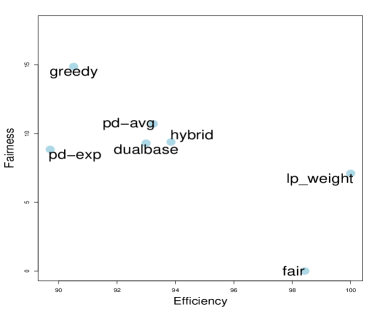
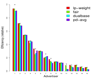
Figure 1: Efficiency and fairness of algorithms for Publisher B (left). Comparison of efficiency of different advertisers for Publisher B (right). Advertisers are sorted by their maximum possible efficiency (given by the inverted triangle).

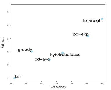
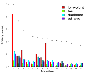
Figure 2: Efficiency and fairness of algorithms for Publisher D (left). Comparison of efficiency of different advertisers for Publisher D (right). Advertisers are sorted by their maximum possible efficiency (given by the inverted triangle).

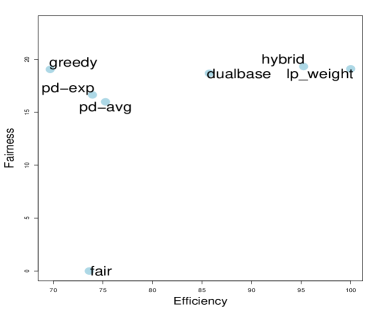
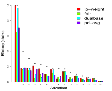
Figure 3: Efficiency and fairness of algorithms for Publisher C (left). Comparison of efficiency of different advertisers for Publisher C (right). Advertisers are sorted by their maximum possible efficiency (given by the inverted triangle).

Experimental Results. The efficiency and (normalized) fairness of the output of each of the algorithms are summarized in Tables 2 and 3. The results for three representative publishers are additionally depicted in Figures  1,  3, and  2. Recall that we normalized efficiency so that the efficiency-optimal algorithm $\mathsf{LP\_WEIGHT}$ has efficiency $100$. Table 2 shows that (1) the training-based algorithms clearly outperform the pure online algorithms, (2) of the pure online algorithms, both $\mathsf{PD\_AVG}$ and $\mathsf{PD\_EXP}$ outperform $\mathsf{GREEDY}$, and (3) $\mathsf{HYBRID}$ and $\mathsf{DualBase}$ perform very similarly, except for one publisher where $\mathsf{HYBRID}$ clearly outperforms $\mathsf{DualBase}$.

Table 3 shows normalized fairness. Since the value of fairness depends on the values assigned to advertisers and different publishers have different advertisers, we normalized the fairness values for each publisher so that the least fair algorithm achieves a score of 100 and algorithm $\mathsf{FAIR}$ achieves a score of 0. Normalizing allows us to compute the average over different publishers. The results in the table indicate that $\mathsf{GREEDY}$ is the least fair algorithm. The remaining algorithms, including $\mathsf{LP\_WEIGHT}$, perform roughly the same, though their performance differs over different publishers.

Figures 1–3 plot efficiency vs. (unnormalized) fairness and they show additionally the efficiency achieved for the top 10 advertisers for four of the algorithms. The inverted triangle above each advertiser represents the maximum possible efficiency for this advertiser if the other advertisers did not exist. There are three rough categories and the publishers for which we show this data each represent a different category: For publisher B in Figure 1 the maximum possible efficiency of the top advertisers is almost the same as the efficiency achieved by all algorithms. This publisher is undersold with little competition between the advertisers. Thus, for this publisher, the choice of algorithm does not heavily influence efficiency. Table 2, shows that for publisher B all algorithms, including $\mathsf{FAIR}$, achieve an efficiency of 90 or above. The situation is similar for publisher A (not shown). In both settings $\mathsf{FAIR}$ has an impressively high efficiency and $\mathsf{LP\_WEIGHT}$ achieves a good fairness value. In such a low-competitive situation the online algorithms are in a clear disadvantage over the offline algorithms. Also the training-based online algorithms outperform the pure online algorithms as they can leverage their knowledge about the data to construct a more efficient and more fair solution.

Publisher D in Figure 2 shows the other extreme: Here the maximum possible efficiency of the top advertisers is much larger than the efficiency achieved by any of the algorithms, including the optimum $\mathsf{LP\_WEIGHT}$. This publisher has a lot of competition between the advertisers. Publisher F (not shown) is in a similar, but a bit less extreme situation. In both cases, the choice of an algorithm has a large influence on the efficiency, as can be seen in Table 2: Algorithm $\mathsf{FAIR}$ distributes the weight more evenly across the advertisers than any of the other algorithms, but also achieves only an efficiency of about 42, resp. 53. Algorithm $\mathsf{LP\_WEIGHT}$, on the other side, generates a very uneven distribution of weights, giving a lot of efficiency to advertiser 1 and 8. For both publishers $\mathsf{PD\_EXP}$ clearly outperforms the non-optimal algorithms. $\mathsf{PD\_EXP}$ also has better theoretical performance.

Finally publishers C (in Figure 3) and E (not shown) represent the “in-between” situation: The maximum possible efficiency of the top advertisers is somewhat larger than the efficiency achieved by the algorithms, but there is not a large gap. In both cases the training-based algorithms clearly outperform the pure online algorithms in efficiency. Thus, this is the situation where learning clearly helps in terms of efficiency.

Overall we draw the following conclusions:

Algorithm $\mathsf{PD\_AVG}$ generally achieves much better efficiency and fairness than $\mathsf{GREEDY}$, even though both algorithms are $1\over 2$-competitive in the worst case. Algorithm $\mathsf{PD\_AVG}$ also results in the best fair solution among all algorithms and $\mathsf{GREEDY}$ has the worst fairness measure.

The training-based algorithms generally achieve higher efficiency than the pure online algorithms, especially in settings that are not too extreme, i.e., oversold or undersold. On average, $\mathsf{DualBase}$ improves 12% over $\mathsf{PD\_AVG}$, and 5% over $\mathsf{PD\_EXP}$. Furthermore, $\mathsf{HYBRID}$ has a marginal improvement (of 2% on average, and upto 10%) over $\mathsf{DualBase}$, mostly based on a big improvement for one publisher.

Though the worst-case competitive analysis of $\mathsf{PD\_EXP}$ is much better than $\mathsf{PD\_AVG}$, this algorithm showed only $5\%$ overall improvement over $\mathsf{PD\_AVG}$, and in one case showed a significant loss in efficiency. However, in highly competitive settings, $\mathsf{PD\_EXP}$ gives large improvements.

6 Concluding Remarks

In this paper, we give a training-based algorithm for online allocation, and prove that in the random-order stochastic model, it achieves a $(1-\varepsilon)$ approximation to the optimal solution under mild assumptions.

We also considered the Display Ad Allocation problem from both a theoretical and empirical perspective, studying fairness in addition to efficiency. We introduced different notions of offline fair allocations, and present a new fairness measure as a distance to such offline fair allocations. Finally, we performed an experimental evaluation of our training-based algorithm, along with previously studied online algorithms and some hybrid algorithms. We compared their performance on data sets from real display ad allocation problems; our experiments show that among the pure online algorithms designed for worst-case inputs, $\mathsf{PD\_AVG}$ performs reasonably well in terms of both efficiency and fairness, and $\mathsf{PD\_EXP}$ gives large improvements for more difficult instances. The training-based algorithm outperforms $\mathsf{PD\_AVG}$ and $\mathsf{PD\_EXP}$ by a large factor, and combining pure online and training-based methods in a hybrid algorithm improves the efficiency further.

This paper motivates many open problems to explore: (i) Can we achieve an algorithm that is simultaneously good both in the worst case and in stochastic settings? Such an algorithm would be of use when the actual distribution of agents is different from the one predicted/learnt from a sample; in the display ad setting, this occurs when there is a sudden spike in traffic to a website, perhaps in response to a breaking news event, or links from an extremely high-traffic source. (ii) Can we design an online allocation algorithm that provably achieves approximate efficiency and approximate fairness (for some an appropriate notion of fairness) at the same time? (iii) Can we prove that in certain settings that appear in practice, the $\mathsf{PD\_AVG}$ algorithm achieves an improved approximation factor (i.e., better than $1\over 2$)? (iv) Can we extend the online stochastic algorithm studied in this paper to other stochastic process models such as Markov-based stochastic models? Answering these questions is an interesting subject of future research.

Acknowledgments. This paper is a followup of our previous work with S. Muthukrishnan and Martin Pál, and some of the results and discussions in this paper are inspired by our initial discussions with them. We thank Martin and Muthu for their contributing insights toward this paper. We also thank the Google display ad team, and especially Scott Benson for helping us with data sets used in this paper.

References

- [1] S. Agrawal, Z. Wang, and Y. Ye. A dynamic near-optimal algorithm for online linear programming. Working paper posted at http://www.stanford.edu/ yyye/.
- [2] S. Alaei and A. Malekian. Maximizing sequence-submodular functions, manuscript. 2009.
- [3] A. Asadpour and A. Saberi. An approximation algorithm for max-min fair allocation of indivisible goods. In STOC, pages 114–121, 2007.
- [4] B. Awerbuch, Y. Azar, and S. Plotkin. Throughput-competitive on-line routing. In FOCS, volume 34, pages 32–40, 1993.
- [5] Y. Azar, B. Birnbaum, A. Karlin, C. Mathieu, and C. Nguyen. Improved Approximation Algorithms for Budgeted Allocations. In ICALP, 2008.
- [6] M. Babaioff, N. Immorlica, D. Kempe, and R. Kleinberg. Online auctions and generalized secretary problems. SIGecom Exchanges, 7(2), 2008.
- [7] N. Bansal and M. Sviridenko. The santa claus problem. In STOC, pages 31–40, 2006.
- [8] M. Bateni, M. Charikar, and V. Guruswami. Maxmin allocation via degree lower-bounded arborescences. In STOC, 2009.
- [9] A. Broder. Introduction to computational advertising, tutorial at wine ’09.
- [10] A. Z. Broder, P. Ciccolo, E. Gabrilovich, V. Josifovski, D. Metzler, L. Riedel, and J. Yuan. Online expansion of rare queries for sponsored search. In WWW, pages 511–520, 2009.
- [11] A. Z. Broder, M. Fontoura, V. Josifovski, and L. Riedel. A semantic approach to contextual advertising. In SIGIR, pages 559–566, 2007.
- [12] N. Buchbinder, K. Jain, and J. Naor. Online Primal-Dual Algorithms for Maximizing Ad-Auctions Revenue. In Proc. ESA, page 253. Springer, 2007.
- [13] N. Buchbinder and J. Naor. Improved bounds for online routing and packing via a primal-dual approach. In FOCS, pages 293–304, 2006.
- [14] D. Chakrabarty, J. Chuzhoy, and S. Khanna. On allocating goods to maximize fairness. In FOCS, 2009.
- [15] D. Chakrabarty and G. Goel. On the approximability of budgeted allocations and improved lower bounds for submodular welfare maximization and GAP. In Proc. FOCS, pages 687–696, 2008.
- [16] S. Chawla, J. D. Hartline, D. Malec, and B. Sivan. Sequential posted pricing and multi-parameter mechanism design. CoRR, To Appear, STOC 2010, 2010.
- [17] F. Chierichetti, R. Kumar, and S. Vassilvitskii. Similarity caching. In PODS, pages 127–136, 2009.
- [18] N. Devanur and T. Hayes. The adwords problem: Online keyword matching with budgeted bidders under random permutations. In ACM EC, 2009.
- [19] J. Feldman, N. Korula, V. Mirrokni, S. Muthukrishnan, and M. Pal. Online ad assignment with free disposal. In WINE, 2009.
- [20] J. Feldman, A. Mehta, V. Mirrokni, and S. Muthukrishnan. Online stochastic matching: Beating 1 - 1/e. In FOCS, 2009.
- [21] A. Ghosh, P. McAfee, K. Papineni, and S. Vassilvitskii. Bidding for representative allocations for display advertising. In WINE, pages 208–219, 2009.
- [22] A. Ghosh, B. I. P. Rubinstein, S. Vassilvitskii, and M. Zinkevich. Adaptive bidding for display advertising. In WWW, pages 251–260, 2009.
- [23] G. Goel and A. Mehta. Adwords auctions with decreasing valuation bids. In WINE, pages 335–340, 2007.
- [24] G. Goel and A. Mehta. Online budgeted matching in random input models with applications to adwords. In SODA, pages 982–991, 2008.
- [25] R. Karp, U. Vazirani, and V. Vazirani. An optimal algorithm for online bipartite matching. In Proc. STOC, 1990.
- [26] J. M. Kleinberg, Y. Rabani, and É. Tardos. Fairness in routing and load balancing. J. Comput. Syst. Sci., 63(1):2–20, 2001.
- [27] R. Kleinberg. A multiple-choice secretary algorithm with applications to online auctions. In Proceedings of the sixteenth annual ACM-SIAM symposium on Discrete algorithms, pages 630–631. Society for Industrial and Applied Mathematics, 2005.
- [28] N. Korula and M. Pal. Algorithms for secretary problems on graphs and hypergraphs. In ICALP, 2009.
- [29] A. Kumar and J. M. Kleinberg. Fairness measures for resource allocation. SIAM J. Comput., 36(3):657–680, 2006.
- [30] R. Lipton, E. Markakis, E. Mossel, and A. Saberi. On approximately fair allocations of indivisible goods. In ACM EC, 2004.
- [31] M. Mahdian, H. Nazerzadeh, and A. Saberi. Allocating online advertisement space with unreliable estimates. In ACM EC, pages 288–294, 2007.
- [32] A. Mehta, A. Saberi, U. Vazirani, and V. Vazirani. Adwords and generalized online matching. In FOCS, 2005.
- [33] S. Pandey, A. Z. Broder, F. Chierichetti, V. Josifovski, R. Kumar, and S. Vassilvitskii. Nearest-neighbor caching for content-match applications. In WWW, pages 441–450, 2009.
- [34] A. Srinivasan. Budgeted Allocations in the Full-Information Setting. In APPROX, 2008.
- [35] A. Vetta. Nash equilibria in competitive societies, with applications to facility location, traffic routing and auctions. In FOCS, 2002.