NSF-KITP-10-010
Semi-Holographic Fermi Liquids
Thomas Faulkner111faulkner@kitp.ucsb.edu and Joseph Polchinski222joep@kitp.ucsb.edu
Kavli Institute for Theoretical Physics
University of California
Santa Barbara, CA 93106-4030
We show that the universal physics of recent holographic non-Fermi liquid models is captured by a semi-holographic description, in which a dynamical boundary field is coupled to a strongly coupled conformal sector having a gravity dual. This allows various generalizations, such as a dynamical exponent and lattice and impurity effects. We examine possible relevant deformations, including multi-trace terms and spin-orbit effects. We discuss the matching onto the UV theory of the earlier work, and an alternate description in which the boundary field is integrated out.
1 Introduction
The existence of non-Fermi liquids, conductors whose gapless charged excitations are not described by the Landau-Fermi liquid effective theory, is a fascinating puzzle in condensed matter physics.111For a recent overview of this subject see Ref. [1]. Even a clear framework is lacking. One approach, the marginal Fermi liquid [2], is a long-standing phenomenology without clear field-theoretic underpinnings. Another, the recent attempt to formulate scaling laws [1], places this subject at the level of development of critical phenomena before the advent of the renormalization group. A third class of ideas, based on emergent gauge theories, presents the difficulty of understanding the resulting strongly coupled dynamics [3].
In this situation, gauge/gravity duality may play a valuable role. Having a large class of solvable quantum field theories provides a theoretical laboratory for understanding phenomena that emerge at strong coupling. This has led to a recent surge of interest in studying duals that capture various features of condensed matter systems; for reviews see Ref. [4].
The known non-Fermi liquids retain a Fermi surface, a surface in momentum space where the electron propagator has IR-singular behavior. In this paper we develop further the duals introduced in Refs. [5, 6, 7, 8], which exhibit such a Fermi surface.222Ref. [9] identifies duals in which a current-current propagator exhibits Fermi-surface-like behavior, although backreaction effects may prevent this from extending fully into the IR [10]. In these duals the sea fermions would be charged under the large- gauge group, whereas in the systems that we consider they are gauge singlets. Ref. [11] identifies some properties of a charged AdS black hole with those of a Fermi gas, but there are no indications of a Fermi surface in the low frequency correlators. In particular, we show that the IR behavior found in Refs. [6, 8] is equivalent to that in a system of dynamical singlet fermions coupled through a fermion bilinear to a strongly coupled conformal sector with dual. We argue that this semi-holographic description has significant advantages: it retains only the universal low energy properties, which are most likely to be relevant to the realistic systems; it allows more flexible model-building; and, it makes it easy to incorporate such features as a spatial lattice and impurities. As an example of the flexibility, we consider the replacement of the holographic sector by systems with other and Lifshitz scalings.
We present this construction in Sec. 2. In Sec. 3 we look at the relevant perturbations of this system, with regard to stability and to the phase diagram. There are a large number of relevant perturbations, multi-trace operators constructed out of the basic fields and currents. These do not appear to destabilize the construction in general. Particular operators, the squares of densities, seem interesting for the phase diagram. We also discuss spin-orbit effects. In Sec. 4 we discuss the matching of the IR theory onto the UV theory of Refs. [6, 8], and we note an interesting renormalization group interpretation of the Fermi surface.
2 Semi-holographic Fermi liquids
Refs. [5, 6, 7, 8] consider 2+1 dimensional conformal theories with a density of conserved charge, whose dual description is a charged black hole. At zero temperature the near-horizon geometry is . In addition there is a charged fermion in the bulk, dual to a charged fermionic operator. In Refs. [6, 8], the Fermi surface of the field theory arises from a sea of these bulk fermions, radially localized on the domain wall separating the UV and IR geometries.
This is interesting from the holographic point of view. The essential low energy degrees of freedom of the system consist of the excitations of the bulk Fermi surface, localized at the domain wall, plus the holographic excitations at the horizon (Fig. 1a). There is also a model-dependent Fermi liquid in the bulk of (Fig. 1b), but this is not connected with the non-Fermi liquid behavior of Refs. [6, 8], so we discuss it later.
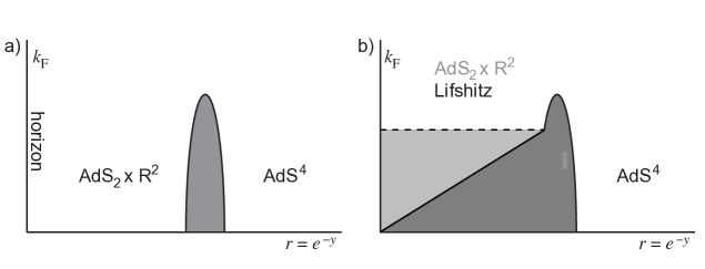
The system shown in Fig. 1a is in the same universality class as a rather different quantum field theory, consisting of free fermions coupled to whatever CFT is dual to the bulk theory. The action is333A similar construction was noted in [8] but not elaborated upon.
| (2.1) |
Here is a charged singlet operator, free aside from the explicit coupling in , is the single-particle energy of the singlet fermions, is the chemical potential, and is an arbitrary coupling function. Also, is a charged fermionic operator from the strongly coupled sector, of dimension , with the spin component. Only the leading behaviors near the Fermi surface are relevant,
| (2.2) |
where is the point on the Fermi surface nearest to , and .
We refer to this construction as semi-holographic: the correlators of the strongly coupled theory are to be calculated via AdS/CFT duality, and then the singlet field integrated explicitly. The singlet couples to local operators in the strongly coupled sector, so is naturally regarded as living on the boundary.444Dynamical boundary fields were introduced in Ref. [12]. Some further developments of this idea are in Refs. [13]. This construction gives a general framework for analyzing the low energy physics of the systems of Refs. [5, 6, 7, 8], while dropping nonuniversal physics. Unlike the phenomenological constructions of bulk duals, here there is an immediate top-down interpretation: given any known dual with a symmetry and charged fermionic operators, we can couple an additional singlet fermion in this way. Further, we are free to consider other scaling behaviors in the strongly coupled sector, such as and Lifshitz spacetimes.
There is no advantage to generating the Fermi sea in the bulk of a larger holographic theory. (In particular, any desire to obtain the fields from an explicit UV brane should be resisted.) Since these fermions are gauge singlets, the geometry does no work for us in summing their quantum effects; if these effects are important we must deal with them ourselves. Further, obtaining both sectors holographically is complicated and constraining. These complications may be essential in determining the low energy physics of a given theory (if a holographic description holds above the scale of the Fermi momentum), but to classify all possible low energy physics within a given universality class the semi-holographic description is more efficient.
As one example of the flexibility of the semi-holographic construction, we can immediately introduce the effects of a spacetime lattice, simply by restricting the momentum of to a unit cell of the reciprocal lattice, with for any reciprocal lattice vector .555For a cubic lattice of side , this restricts the momentum components to with periodic boundary conditions. The coupling to the strongly coupled sector must be generalized to
| (2.3) |
This allows transfer of momentum to the lattice, as is essential to the DC resistivity [14]. Similarly, we can introduce impurities, by adding to the action and/or terms that violate momentum conservation.666For other approaches to lattices and impurities see Refs. [15, 16] respectively.
To leading order in , the action for the bulk fermion dual to the operator is quadratic, and so the coupled action for and is quadratic. Thus we can immediately calculate the correlators. In fact, we can do this directly in the quantum theory, though the bulk description would be needed to obtain transport and thermal properties. We use and respectively for the and correlators. The decoupled Feynman correlators are
| (2.4) |
where the subscripts indicate that has been set to zero. The dependence of is determined by scale invariance; this becomes at . The coefficient is obtained by a holographic calculation in the IR theory [8, 17] for the case of with an electric field in . The magnitude of depends on convention, but there is phase which is physical.777We are neglecting possible spin-orbit coupling terms in the action (2.1), so as not to distract from the main point of the following discussion. In Sec. 3.3 we introduce these terms, which are necessary to match to the original model. Because of these spin-orbit effects and may be matrices in the spin basis, which we suppress for now.
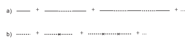
Expanding in powers of , and using the factorization property of large- correlators, the propagator is (Fig. 2)
| (2.5) | |||||
exhibiting the strange metallic behavior discussed in Refs. [6, 8]. The calculation uses only the factorization property and so would be equally true in weakly coupled large- theories.
Now we can see what happens if the strongly coupled theory is replaced by an theory, with an operator of dimension in the dimensional CFT. The correlator
| (2.6) |
implies
| (2.7) |
with . Since the Fermi momentum is a UV scale we are interested in and so we expand,
| (2.8) |
Using this in the correlator (2.5), the leading -independent term should be absorbed into the definiton of from the UV theory. The leading correction to the fermion self-energy is as in Fermi liquid theory, but here it is real because the kinematics forbids the quasiparticle decay. This example should capture the low energy dynamics of the models considered in [18] where a fermion lives in a zero temperature holographic superconducting background and the IR part of the geometry was an emergent solution.
Similarly, we can extend to a Lifshitz theory with dynamical exponent . For an operator of energy dimension ,
| (2.9) |
This asymptotic expansion in is seen, for example, in the holographic calculation of the correlator [19], obtained by solving the differential equation
| (2.10) |
Here we have for simplicity taken a scalar correlator to illustrate the scaling, in the metric
| (2.11) |
and we have defined , . At , the term is dominant at the horizon, giving the normalizable solution . Perturbation theory in is nonsingular order by order because this solution falls off rapidly at large , so again the leading correction scales as in Fermi liquid theory, but with a real coefficient.
The fermionic correlator will have similar scaling properties. Thus, the non-Fermi liquid behavior found in Refs. [6, 8] is only present for the IR theory, in which the momentum does not scale. The fermionic correlator would have interesting properties when and are both small, but this does not affect the Fermi surface behavior. Also, when there is bulk Fermi sea as in Fig. 1b, the dimension becomes complex, but again this is seen only when and become small together.
Let us discuss a few more aspects of the Lifshitz case. For finite values of , the term dominates at the horizon and the boundary conditions are changed to . The quasiparticle width is a tunneling effect and can be estimated using the WKB approximation, where
| (2.12) |
and is a UV cutoff. At small frequency the barrier is large, and we can approximate . We can neglect the terms and send the UV cutoff to infinity to find,
| (2.13) |
The imaginary part goes to zero exponentially at low frequency.
It is interesting to examine the crossover from Lifshitz to behavior as becomes large ( corresponding to ). To do this we expand around the answer for , which can also be read off from the WKB approximation:
| (2.14) |
where . For large the turning point is . We can expand the integrand in as long as the term is subdominant over the domain of the integral. This is the case for such that now the quasi particle width behaves as,
| (2.15) |
We have recovered the scaling with log corrections and scaling dimension . The ’s will be small for . For energy scales the answer will then cross over to (2.13). Thus for modestly large values of the strange metal behavior extends down to very low energies with small logarithmic corrections.
The Lifshitz case studied above should apply to the low energy dynamics of fermions introduced into various known gravity backgrounds with Lifshitz as the IR fixed point. Examples are the charged dilaton black holes considered in [20] and the extremal limit of some holographic superconductors [21], though some details will be slightly different. For example the quasiparticle width will now depend on the charge of the fermion due to the radial electric field in these backgrounds. We expect the limit of the models in [20] will recover many of the details of the theory including the scaling exponent given in Eq. (4.5), hence they deserve more detailed study.
When the dimensions in the case lie partly on the conformal branch where is imaginary, a Fermi sea also develops in the region. The backreaction from this sea changes the geometry to the Lifshitz form, with a dynamical exponent that is large in the planar limit of the strongly coupled theory [10]. Over most of the parameter space of Ref. [8] this low energy Fermi sea accompanies the domain wall Fermi sea, though there is a small range of parameters where the latter is absent (this will be discussed in Section 4 in more detail). From the semi-holographic point of view here, the bulk and boundary Fermi seas are independent features.
The marginal Fermi liquid phenomenology [2] also involves a Fermi sea coupled to an -like sector, the latter having correlators that are singular at for all . In the present work, however, the two sectors are coupled through a fermion mixing interaction, whereas in the marginal Fermi liquid they are coupled through bosonic operators.
In the strongly coupled CFT, the operator is a composite of the fundamental fields. Thus the semi-holographic Fermi liquid has a natural interpretation describing charge carriers that have some amplitude to be pointlike and some amplitude to fragment. Such fragmentation plays a major role in many attempts to understand exotic phases [22]. It is interesting that in the present construction this fragmentation is only possible with scaling. The electrons near the Fermi surface have large momentum, and so, except in the case that momentum does not scale, their fragments are far off shell and cannot separate substantially.
If the electron does fragment, it is natural to ask what it fragments into. In the supergravity limit there is no answer to this question, because the field theory is very strongly coupled (large ’t Hooft coupling).888The term ‘quasiparticle’ is used in condensed matter for any particle-like excitation in a low energy effective theory, like the charge carriers in Fermi liquid theory. The term ‘unparticle’ (or, better, ‘unparticle stuff’) is used in some circles [23] for the excitations in strongly coupled scale invariant theories. Thus one could say that the electron fragments into ‘unquasiparticles,’ or perhaps ‘quasiunparticles.’ This is one of the difficulties in applying gauge/gravity duality to QCD: the partonic structure is not seen. Fortunately there is a wealth of phenomena in heavy ion physics where the partons are not relevant and the ’t Hooft coupling is of order one. In the condensed matter case, in the 2+1 dimensional systems where fragmentation is most often considered, the gauge coupling again is of order one. The details of the partons may therefore not be so important — indeed, there may be several equally valid dual descriptions. Thus the situation may not be so different from that in heavy ion physics.
Having a fundamental fermion coupled to the composite would appear to be a new ingredient outside the usual fragmentation picture. In Sec. 3.1 we will show that in the interesting range of parameters can be integrated out.
3 Relevant operators
Relevant operators are important for two reasons: they can make the low energy physics unstable to generic quantum corrections, and they affect the phase diagram as parameters are varied. The phase diagram of the cuprates appears to be controlled by a single relevant operator, tied to the doping.999The doping appears directly in the action (2.1) through the chemical potential , but integrating out the high energy degrees of freedom will make all other parameters implicit functions of . Writing the action (2.1) explicitly in terms of is therefore somewhat deceptive. Rather, the low energy kinetic term depends on the locus of (the Fermi surface) and on the normal derivative of the energy, , both of which are functions of . We will see this explicitly when mapping to the theory in section 4. At large doping , the zero temperature behavior is that of a Fermi liquid, and non-Fermi liquid behavior sets in at a temperature . As the doping is reduced to a critical value , comes down close to zero (when the superconducting phase is suppressed). Below there is a mysterious phase with possible charge and spin inhomogeneities.
As we will see, the theory we are discussing necessarily has an abundance of relevant operators. However, the low energy physics is stable, within a range of parameters. We also identify operators which may play the needed role in the phase diagram.
3.1 Fermionic bilinears
Candidate operators are the various bilinears, , , , and .
From the action (2.1) it follows that has energy dimension zero and so is relevant. However, this term is already present in the action: perturbing its coefficient just moves the Fermi surface, but does not destroy it. Similarly the operators and are already included with generic coefficients. Their dimension is , and so they are relevant for . This is just the regime where the correlator (2.5) exhibits strange behavior (the marginal case is also of interest).
For genericity we should also add
| (3.1) |
This is relevant when . Such double-trace perturbations have been considered in Refs. [24, 25, 26, 27, 28]. To see their effect, consider first the decoupled theory at . As in the calculation of the propagator (2.5), we can sum the perturbations at planar order to get
| (3.2) |
where again . In the irrelevant range , the perturbed correlator approaches at low energy. However, for the low energy limit is
| (3.3) |
The first term is a contact interaction and can be absorbed into the parameters in the action. The second, which is the leading nonlocal term, scales as . The relevant perturbations thus leave a critical theory but shift the dimension to [25, 29]. The fine-tuned theory with which we began is known as the alternate quantization, and it flows to the standard quantization. The low energy physics is the same as would have been obtained using , the standard quantization, from the start.
In summary, the effect of generic fermionic bilinears is simply to restrict the dimensions to , but otherwise leave the low energy physics as before. These bilinears do not seem suitable for controlling the behavior of the phase diagram. In particular, the different directions on the Fermi surface do not talk to each other, at least in the planar limit, and their coefficients are independent. Thus it is difficult to see how they can account for a single relevant operator that drives the entire Fermi surface critical at once, as indicated by the existence of a sharp .
We present one more manipulation along these lines, which gives an interesting interpretation to the non-Fermi surface. We can integrate out the singlet fermion and express the result as a boundary condition on the bulk theory. This would usually be nonlocal, because of the time derivative term in the action. However, when one sees from the propagator (2.5) that the time derivative is is less relevant than the interaction with the bulk. We can therefore ignore it at low energy, so that is effectively nondynamical. Integrating out then gives the action
| (3.4) |
Assuming that we start with the standard quantization, the pole implies that on the Fermi surface we have transformed to the alternate quantization. To see this, we evaluate the correlator by using the result (3.2) with given by Eq. (3.4):
| (3.5) |
The second term in the denominator scales as . Thus, for this term dominates and the propagator is approximately given by a contact term plus a term that has the alternate scaling. Below this frequency the correlator crosses over to the standard scaling. As we approach the Fermi surface the crossover frequency goes to zero and the alternate quantization applies down to the IR (though with an overall normalization on the correlator that goes to zero). See also Fig. 3 and the discussion at the end of Section 4.1.
3.2 Density multilinears
In this paper we are considering only universal properties of theories whose IR physics includes the system (2.1). In addition to the fermionic operators , this will include the energy momentum tensor and the density and current , under which is charged. In the theory, the density has dimension zero: the dual CFT is 0+1 dimensional, and so the current has the same scaling as the charge. The spatial derivatives also do not scale. Therefore any function of and is relevant [10]. This is an embarrassment of riches, and may lead one to doubt that an fixed point can ever be realized. However, in the planar limit the RG flows induced by multi-trace operators (functions of gauge-singlet operators) are rather tame [25, 26, 27, 28].101010These perturbations are nonlocal in the compact directions of the bulk dual [24], but this does not lead to any pathologies. The theory flows to a new fixed point with the same conformal symmetry, and only the correlator of the perturbed operator is affected.
We should also consider the single-trace operators as a potential relevant perturbations. We consider first the case that this is forbidden by a symmetry and the double-trace is the leading relevant term. This is somewhat unnatural for the charge density, though it may apply to spin density as we discuss in Sec. 3.3. In 3.2.2 we look at the single-trace perturbation.
3.2.1 Density bilinears
Let focus on a density-squared perturbation,
| (3.6) |
Higher powers of the density are also relevant but do not affect the two-point correlator in the planar limit. The dimension zero case is rather degenerate, so let us consider a general Lifshitz exponent . As we reduce the number of relevant interactions decreases, the energy dimension of the current being and the condition for relevance being total dimension less than . Thus the density-squared perturbation is relevant for [10] (the marginal case is left for the reader). The charge density-density correlator in the strongly coupled theory is of the form
| (3.7) |
The same summation that gave the fermion propagator (2.5) gives the full density-density correlator
| (3.8) |
For this flows to the unperturbed (3.7). However, for the low energy behavior is
| (3.9) |
The leading piece is a contact term. The leading nonlocal behavior corresponds to the dimension of the density being shifted to , and so the density-density perturbation around this new fixed point is irrelevant.
This is suggestive. At positive the charge fluctuations in the IR have a certain behavior. When is reduced to zero, these fluctuations become stronger in the IR. Once goes negative, the correlator has a pole at nonzero for zero , indicating an instability. The enhanced fluctuations at may be connected with the critical behavior. If so, this is a somewhat conventional picture [30]. The holography is playing a role in determining the correlators in the strongly coupled theory, where the density fractionalizes [31] as in the earlier discussion. (One might hope that the bulk description will determine the endpoint of the instability, although the details here are not clear). However, in the end we must treat by hand the interactions between the singlet fluctuations and the fermions, unless we can find a more effective dual theory.
As a technical point, it might seem puzzling that a density such as could acquire an anomalous dimension, because the Ward identity appears to fix its dimension via the OPE
| (3.10) |
One can perturb the terms in this relation as we have done above, with the result
| (3.11) |
The Ward identity is still satisfied, but for the makes no contribution in the IR and so the dimension of is not constrained. Rather, the term, representing an outflow of charge at spatial infinity, appears in the IR and allows the spatial current term by itself to saturate the Ward identity. One can give this a physical interpretation as follows. In Ref. [10], it was noted that the IR stable quantization for forbids local fluctuations of the charge density (where in the present discussion charge is replaced by spin). When a nonsinglet operator such as acts to create a local density, this must be accompanied by an outflow at infinity.
3.2.2 Linear density terms
The current is always relevant according to the standard dimensional analysis, given below Eq. (3.6). This would have a large effect on the IR: the strongly coupled CFT has charged excitations of arbitrarily low energy, so adding a bulk chemical potential to the action will induce a density of these charges. In fact, in the and Lifshitz geometries of [20] this density should already be present: the geometry is sourced by a charged horizon, and the Lifshitz geometry in [20] is sourced by a charge density in the bulk. (We could consider models with multiple ’s, but here we are looking only at the simplest case).
Thus we should expand
| (3.12) |
The leading contribution to the current is proportional to a -number in the IR. Assuming that the classical or Lifshitz solution is an IR attractor, the leading operator contribution will be irrelevant. When there is a bulk charge density, the mass of the bulk photon is lifted by Higgsing or plasma effects, and with it the dimension of . In the case, with the Einstein-Maxwell action, mixing between the photon and the metric lifts the dimension of to 2.
We present here the derivation of this last result. We take the background Ansatz
| (3.13) |
with vector potential . The Einstein-Maxwell field equations (in units where the coupling is 1) are
| (3.14) | |||||
a dot denotes . Linearizing around the solution,
| (3.15) |
the field equations become
| (3.16) | |||||
in terms of the derivatives . The two solutions
| (3.17) |
scale respectively as the normalizable and nonnormalizable modes for in a 1+0 dimensional CFT. This should be compared to the universal result on the anomalous scaling dimension of the vector part of the current at zero momentum: , found in [32] and studied further in the transverse channel at non-zero momentum in [33]. The non-zero analysis for the longitudinal part of the current would be valuable to compare to the above result.
In summary, there is generically no charge density of canonical dimension in the IR CFT, and the Ward identity must be satisfied without it as in the discussion in Sec. 3.2.1. Perturbations involving the density in the UV do not destabilize the IR physics, with one notable exception: the relativistic case is unnatural for a CFT with a charge, because the relativistic symmetries are broken by any charge density.
3.3 Spin-orbit coupling
There is another set of relevant operators that we can add to (2.1) which we have thus far neglected. These are the spin-orbit Rashba [34] terms,
| (3.18) |
where are the usual Pauli matrices in the spin basis . These terms respect two-dimensional parity, as compared to a term such as as which does not.111111Recall that parity in two space dimensions is defined by reflection about a single axis, and as usual is a pseudovector under this parity. For a two-dimensional system embedded in three dimensions, the Rashba interaction arises from an interaction . Treating as a vector, this respects the underlying parity symmetry but requires a spontaneous breaking of reflection symmetry in the third direction, for example by the crystal structure. When this symmetry is broken these terms can have interesting physical consequences [35].
Allowing the terms (3.18) will be important for us because they are present in the theory, and must be included in order to match to that theory. In that case the reflection symmetry in the third direction is broken by the warped geometry. In particular, as we will explain below, because the strongly coupled field naturally does not respect this “reflection” symmetry it would constitute a fine tuning not to include these terms.
We can diagonalize the full action in terms of the eigenbasis under reflection perpendicular to the momentum,
| (3.19) |
where is the phase of . This is the basis that Ref. [8] works in. Then,
| (3.20) |
where,
| (3.21) |
This term splits the degenerate Fermi surfaces labeled by spin into two non degenerate fermi surfaces labeled by . For example in this basis the generalization of (2.5) is found by replacing with . Note that time reversal is still preserved, and simply maps to .
In addition, in this basis the correlator coming from the strongly coupled sector for the field will be diagonal since we demand that the strongly coupled field theory respects and . That is in (2.5) we should replace . There is no reason for this sector to respect the “reflection” symmetry discussed above, thus and in the original spin basis the correlator will not be diagonal. Note that in the supergravity approximation the dimension of is independent of , but no symmetry appears to require this at higher order.
Aside from the reflection symmetry, spin-orbit interactions are also forbidden in the extreme nonrelativistic limit, where emerges as an accidental symmetry (as in heavy quark systems). This is often treated as an effective internal symmetry in condensed matter systems. Thus we might model it by introducing an explicit index on the fermionic fields; this could be the original in Eq. (2.1), with the additional index inherited from the bulk field suppressed. There will be a small symmetry breaking, from the combination of lattice and spin-orbit effects.
One would then expect that the approximately conserved current would be holographically realized as an gauge symmetry in the bulk, weakly broken. The discussion of density bilinears above would extend to the spin density, where the absence of a single-trace term would usually follow from dicrete symmetries.
We can attempt to include some more physics, in particular the fact that the spin fluctuations may be strongest at the antiferromagnetic point. We thus introduce a lattice as before, elaborating the perturbation to
| (3.22) |
The resulting correlator is
| (3.23) |
where
| (3.24) |
In an antiferromagnetic system the coupling would be negative at some nonzero momentum. However (as with the earlier discussion of behavior at the Fermi surface), for any finite the interesting critical behavior in the bulk is at zero momentum and does not seem to affect the antiferromagnetic point. Perhaps we have not introduced the lattice physics in the most general way. One further possibility would be the introduction of constant gauge fields in the bulk.
4 Matching onto the UV theory
In general, the system we have been discussing will describe the low energy physics of some higher energy QFT in 2+1 dimensions. The UV theory has some leading fermionic operator which is represented in the CFT as
| (4.1) |
where the omitted terms include time derivatives, multitraces, and so on. Since has dimension 0 and dimension at least , the leading low energy behavior of the correlator comes from the former, and so from the IR correlator (2.5) generalized to the basis we have
| (4.2) |
In the remainder of this section we focus on the case that the UV theory is the original theory studied in Refs. [5, 6, 7, 8]. We will suppress the index wherever possible to avoid clutter.
4.1 Matching onto the theory
The bulk geometry is the (extremal) RN black hole. As a function of the radial coordinate this geometry represents the RG flow of the field theory triggered by turning on the relevant charge density operator in the UV. At scales much smaller than the theory flows to the theory, where now represents a UV cutoff. It seems reasonable to assume that the low energy theory is universally controlled by the theory plus the domain wall singlet fermions. Here we explore this interpretation.
The fermionic operator in the UV CFT can be considered with general scaling dimension and charge . The fermionic correlators can be written as [8],
| (4.3) |
where
| (4.4) |
and are only calculable numerically order by order in perturbation theory. The IR dimension is fixed by the specific theory to be [8],
| (4.5) |
where is an order one number fixed by the normalization of the current two point function. It would be useful to understand how robust this relation is, or whether there are other theories which give different scaling dimensions.
As discussed in [8] the condition for the appearance of a Fermi surface is . Expanding at low energy, this matches the general result (4.2) up to a contact term, with the identifications
| (4.6) |
To reproduce higher order terms in (4.3) we would have to include general time derivatives in the expansion (4.1), and also go to higher order in the expansion (2.2) of the low energy action.
For the observation at the end of section 3.1 gives a nice picture of the RG flow represented by the theory. Since we can now ignore the free field in favor of the interacting field in the IR CFT, we can match directly onto the theory via the strongly interacting fermionic operator in that theory;
| (4.7) |
We must also specify the presence of an irrelevant double-trace deformation as in (3.4),
| (4.8) |
after which the correlator is given by the earlier result (3.5).
It is natural that under RG flow all multi-trace relevant operators in the IR theory not protected by a symmetry should be turned on. Hence we expect naturally the IR theory is in its standard quantization. However, we have seen in Sec. 3.1 that it is precisely on the Fermi surface that we are tuned to the alternate quantization, and the IR fluctuations are enhanced. Generically this tuning will happen on a codimension one surface in momentum space. As we move away from the Fermi surface, the alternate quantization holds only down to a crossover scale .
This interpretation is depicted in Fig. 3. We flow in the UV theory (denoted ) to the theory at the UV end of the IR CFT (denoted ). This IR CFT has an infinite number of double-trace couplings, indexed by . For near the Fermi surface, the coupling lingers for a long time near the unstable fixed point corresponding to the alternate quantization, while values of further from the Fermi surface cross over sooner.

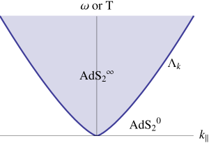
The CFT with alternative quantization is controlling the physics of the Fermi surface. This interpretation explains the universal behavior recently found for the transport [17] and thermodynamics [36, 37] of this model when .
Such an interpretation for is hampered by the now relevance of the time derivative term in (2.1). Thus the low energy effective theory is no longer just the theory. Indeed, close to the fermi surface the theory is now controlled by the free fermion .
It would be interesting to match the low energy gauge field sector of the theory to the discussion of bosonic bilinears in the last section. This may help to track the instability identified for the density bilinear. We leave this to future work.
4.2 Relevant and irrelevant deformation of the theory
The space of possible low energy theories (2.1) that can be constructed with this theory was examined in Ref. [8]. Here we generalize these results by allowing for double-trace fermion operators in the theory. We start by considering relevant operators, noting that there is potentially another natural candidate for the doping. However we then note that since the UV CFT is not governing the low energy physics the distinction between irrelevant and relevant in the UV is immaterial. Both should alter the low energy physics only through their effect on the already identified relevant operators in the low energy effective action (2.1). In particular the cutoff scale above which the theory is important should be at the same scale as the lattice scale and as such we should include possible lattice effects. We only briefly explore this possibility.
We will restrict our attention to the region where the bulk fermi sea does not back react on the geometry as in [10]. This condition is equivalent to requiring is real for all , or
| (4.9) |
This corresponds to the regions of Fig. 6 of Ref. [8] below the dashed lines. There are only zeros (shaded areas in that figure) of in the bottom left wedge of the component (and none in the component.) This is when and ; which is exactly the critical region of the theory and in the alternative quantization of the theory. This means from the UV theory perspective there are relevant double-trace operators which when turned on will induce a flow to a theory without a Fermi surface [8]. Here we extend this observation and note that this flow is quite interesting, in particular how the Fermi surface disappears depends on the sign of the double-trace coupling. More specifically we will add to the action the following,
| (4.10) |
which is like a chemical potential for distinct from . Note one could also add the relevent, Lorentz invariant term , but this violates and in dimensions, so we will not include it. We will consider the dimensionless quantity .
Suppressing dependence, we can sum the double-trace perturbations as before,
| (4.11) |
There is now a zero-frequency pole of the propagator at
| (4.12) |
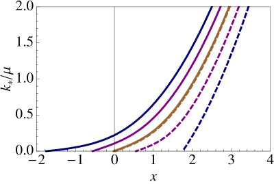
As increases the fermi momentum increases and diverges as . Decreasing the fermi surface vanishes beyond some point . Indeed may be a candidate for the doping although no new critical behavior will happen as a function of and there is nothing to single out as special.
In Figure 4 some flows under were constructed explicitly with the theory. Note that the exponent increases as a function of ; for fixed it now varies from , a much larger parameter space than discussed earlier. It is interesting to note from the middle curve in Figure 4, which has , that there can now exist fermi surfaces (of non-zero size) when the fermion is uncharged. Also for the spin orbit terms (3.18) are naturally zero, presumably due to a particle-hole symmetry. One thing to take away from this section is that the size of the Fermi surface in the model can be tuned independently of . This will be useful in isolating and studying the thermodynamic properties of the Fermi surface, including their response to an external magnetic field already studied in [37, 38].121212We thank Hong Liu for emphasizing this point.
Notice there is nothing special about the point . The reason for this is the UV CFT is not controlling the physics of the fermi surface. Indeed since is at the same scale as the cutoff scale , the lattice size should also be at the scale . So there is no reason not to include general irrelevant and relevant deformations at this scale, ones that break translation and rotation invariance, to mimic the effects of a lattice. This is easier to achieve using double-trace deformations, although there is no reason to not turn on single-trace operators; it is just much harder to analyze.
Consider adding to the theory the deformation but now modulated on the scale of the lattice, . Then the two point function can be shown to be,
| (4.13) |
As above we can match this theory onto (2.1) where we must now restrict the momentum to the unit cell of the reciprocal lattice, and allow for a coupling as in (2.3). For example the condition for a fermi surface is,
| (4.14) |
Hence this construction sits within the universality class of low energy theories in (2.1). Although this construction on its own might be useful for analyzing the transport and thermodynamic properties of (2.1).
Acknowledgments
We would like to thank S. Hartnoll, N. Iqbal, H. Liu, J. McGreevy, E. Silverstein, D. Tong, and D. Vegh for extensive discussions and collaboration on related questions. We also thank L. Balents, S. Kachru, H. Katsura, V. Kumar and M. Roberts for useful discussions and E. Silverstein for suggestions on the manuscript. JP is grateful to the Institute for Advanced Studies for hospitality while part of this work was carried out. This work was supported in part by NSF grants PHY05-51164 and PHY07-57035 and the UCSB physics department.
References
- [1] T. Senthil, “Critical fermi surfaces and non-fermi liquid metals,” Phys. Rev. B 78, 035103 (2008) [arXiv:0803.4009 [cond-mat.str-el]].
- [2] C. M. Varma, P. B. Littlewood, S. Schmitt-Rink, E. Abrahams and A. E. Ruckenstein, “Phenomenology of the normal state of Cu-O high-temperature superconductors,” Phys. Rev. Lett. 63, 1996 (1989).
- [3] Sung-Sik Lee, “Low energy effective theory of Fermi surface coupled with U(1) gauge field in 2+1 dimensions,” Phys. Rev. B 80, 165102 (2009) [arXiv:0905.4532 [cond-mat.str-el]], and references therein.
- [4] S. A. Hartnoll, “Lectures on holographic methods for condensed matter physics,” arXiv:0903.3246 [hep-th]; C. P. Herzog, “Lectures on holographic superfluidity and superconductivity,” J. Phys. A 42, 343001 (2009) [arXiv:0904.1975 [hep-th]]; J. McGreevy, “Holographic duality with a view toward many-body physics,” arXiv:0909.0518 [hep-th]; S. A. Hartnoll, “Quantum critical dynamics from black holes,” arXiv:0909.3553 [cond-mat.str-el].
- [5] S. S. Lee, “A Non-Fermi Liquid from a Charged Black Hole: A Critical Fermi Ball,” arXiv:0809.3402 [hep-th].
- [6] H. Liu, J. McGreevy and D. Vegh, “Non-Fermi liquids from holography,” arXiv:0903.2477 [hep-th].
- [7] M. Cubrovic, J. Zaanen and K. Schalm, “Fermions and the AdS/CFT correspondence: quantum phase transitions and the emergent Fermi-liquid,” arXiv:0904.1993 [hep-th].
- [8] T. Faulkner, H. Liu, J. McGreevy and D. Vegh, “Emergent quantum criticality, Fermi surfaces, and AdS2,” arXiv:0907.2694 [hep-th].
- [9] M. Kulaxizi and A. Parnachev, “Holographic Responses of Fermion Matter,” Nucl. Phys. B 815, 125 (2009) [arXiv:0811.2262 [hep-th]]; “Comments on Fermi Liquid from Holography,” Phys. Rev. D 78, 086004 (2008) [arXiv:0808.3953 [hep-th]].
- [10] S. A. Hartnoll, J. Polchinski, E. Silverstein, and D. Tong, “Towards strange metallic holography,” arXiv:0912.1061 [hep-th].
- [11] S. J. Rey, “String Theory On Thin Semiconductors: Holographic Realization Of Fermi Points And Surfaces,” Prog. Theor. Phys. Suppl. 177, 128 (2009) [arXiv:0911.5295 [hep-th]].
- [12] E. Witten, “SL(2,Z) action on three-dimensional conformal field theories with Abelian symmetry,” arXiv:hep-th/0307041.
- [13] R. G. Leigh and A. C. Petkou, “SL(2,Z) action on three-dimensional CFTs and holography,” JHEP 0312, 020 (2003) [arXiv:hep-th/0309177]; H. U. Yee, “A note on AdS/CFT dual of SL(2,Z) action on 3D conformal field theories with U(1) symmetry,” Phys. Lett. B 598, 139 (2004) [arXiv:hep-th/0402115]; D. Marolf and S. F. Ross, “Boundary conditions and new dualities: Vector fields in AdS/CFT,” JHEP 0611, 085 (2006) [arXiv:hep-th/0606113]; R. G. Leigh and A. C. Petkou, “Gravitational Duality Transformations on (A)dS4,” JHEP 0711, 079 (2007) [arXiv:0704.0531 [hep-th]]; J. V. Rocha, JHEP 0808, 075 (2008) [arXiv:0804.0055 [hep-th]]; G. Compere and D. Marolf, Class. Quant. Grav. 25, 195014 (2008) [arXiv:0805.1902 [hep-th]].
- [14] N.W. Ashcroft and N.D. Mermin, Solid State Physics (Holt, Rinehart and Winston, New York 1976).
-
[15]
S. Hellerman,
“Lattice gauge theories have gravitational duals,”
arXiv:hep-th/0207226;
S. Kachru, A. Karch and S. Yaida, “Holographic Lattices, Dimers, and Glasses,” arXiv:0909.2639 [hep-th]. - [16] S. A. Hartnoll and C. P. Herzog, “Impure AdS/CFT,” Phys. Rev. D 77, 106009 (2008) [arXiv:0801.1693 [hep-th]].
- [17] T. Faulkner, N. Iqbal, H. Liu, J. McGreevy and D. Vegh, in preparation.
- [18] T. Faulkner, G. T. Horowitz, J. McGreevy, M. M. Roberts and D. Vegh, “Photoemission ‘Experiments’ on Holographic Superconductors,” arXiv:0911.3402 [hep-th]. S. S. Gubser, F. D. Rocha and P. Talavera, “Normalizable Fermion Modes in a Holographic Superconductor,” arXiv:0911.3632 [hep-th]. J. W. Chen, Y. J. Kao and W. Y. Wen, “Peak-Dip-Hump from Holographic Superconductivity,” arXiv:0911.2821 [hep-th].
- [19] S. Kachru, X. Liu and M. Mulligan, “Gravity duals of Lifshitz-like fixed points,” Phys. Rev. D 78, 106005 (2008) [arXiv:0808.1725 [hep-th]].
- [20] K. Goldstein, S. Kachru, S. Prakash and S. P. Trivedi, “Holography of Charged Dilaton Black Holes,” arXiv:0911.3586 [hep-th].
- [21] S. S. Gubser and A. Nellore, “Ground States of Holographic Superconductors,” Phys. Rev. D 80 (2009) 105007 [arXiv:0908.1972 [hep-th]]. G. T. Horowitz and M. M. Roberts, “Zero Temperature Limit of Holographic Superconductors,” JHEP 0911 (2009) 015 [arXiv:0908.3677 [hep-th]].
- [22] P. W. Anderson, “When the electron falls apart,” Phys. Today 50N10, 42 (1997).
- [23] H. Georgi, “Unparticle Physics,” Phys. Rev. Lett. 98, 221601 (2007) [arXiv:hep-ph/0703260].
- [24] O. Aharony, M. Berkooz and E. Silverstein, “Multiple-trace operators and non-local string theories,” JHEP 0108, 006 (2001) [arXiv:hep-th/0105309].
- [25] E. Witten, “Multi-trace operators, boundary conditions, and AdS/CFT correspondence,” arXiv:hep-th/0112258.
- [26] M. Berkooz, A. Sever and A. Shomer, “Double-trace deformations, boundary conditions and spacetime singularities,” JHEP 0205, 034 (2002) [arXiv:hep-th/0112264].
- [27] S. S. Gubser and I. Mitra, “Double-trace operators and one-loop vacuum energy in AdS/CFT,” Phys. Rev. D 67, 064018 (2003) [arXiv:hep-th/0210093].
- [28] S. S. Gubser and I. R. Klebanov, “A universal result on central charges in the presence of double-trace deformations,” Nucl. Phys. B 656, 23 (2003) [arXiv:hep-th/0212138].
- [29] I. R. Klebanov and E. Witten, “AdS/CFT correspondence and symmetry breaking,” Nucl. Phys. B 556, 89 (1999) [arXiv:hep-th/9905104].
-
[30]
J. A. Hertz, “Quantum critical phenomena,”
Phys. Rev. B 14, 1165 (1976);
T. Moriya, Spin Fluctuations in Itinerant Electron Magnetism, Springer- Verlag, Berlin (1985);
A. J. Millis, “Effect of a nonzero temperature on quantum critical points in itinerant fermions systems,” Phys. Rev. B, 48, 7183 (1993). - [31] T. Senthil, A. Vishwanath, L. Balents, S. Sachdev, and M. P. A. Fisher, “Deconfined quantum critical points,” Science 303, 1490 (2004).
- [32] M. Edalati, J. I. Jottar and R. G. Leigh, “Transport Coefficients at Zero Temperature from Extremal Black Holes,” arXiv:0910.0645 [hep-th]. M. F. Paulos, “Transport Coefficients, Membrane Couplings and Universality at Extremality,” arXiv:0910.4602 [hep-th]. R. G. Cai, Y. Liu and Y. W. Sun, “Transport Coefficients from Extremal Gauss-Bonnet Black Holes,” arXiv:0910.4705 [hep-th]. S. Jain, “Holographic Electrical and Thermal Conductivity in Strongly Coupled Gauge Theory with Multiple Chemical Potentials,” arXiv:0912.2228 [hep-th].
- [33] M. Edalati, J. I. Jottar and R. G. Leigh, “Shear Modes, Criticality and Extremal Black Holes,” arXiv:1001.0779 [hep-th].
- [34] Bychkov, Y. A. and Rashba, E. I, “Properties of a 2D electron gas with lifted spectral degeneracy,” Sov. JETP. Lett., (1984), Vol. 39, p78
- [35] J. Sinova, D. Culcer, Q. Niu, N. A. Sinitsyn, T. Jungwirth, A.H. MacDonald. “Universal Intrinsic Spin-Hall Effect,” Phys. Rev. Lett. 92, 126603 (2004).
- [36] S. A. Hartnoll and D. M. Hofman, “Generalized Lifshitz-Kosevich Scaling at Quantum Criticality from the Holographic Correspondence,” arXiv:0912.0008 [cond-mat.str-el].
- [37] F. Denef, S. A. Hartnoll and S. Sachdev, “Quantum Oscillations and Black Hole Ringing,” arXiv:0908.1788 [hep-th]. F. Denef, S. A. Hartnoll and S. Sachdev, “Black Hole Determinants and Quasinormal Modes,” arXiv:0908.2657 [hep-th].
- [38] P. Basu, J. He, A. Mukherjee and H. H. Shieh, “Holographic Non-Fermi Liquid in a Background Magnetic Field,” arXiv:0908.1436 [hep-th]. T. Albash and C. V. Johnson, “Holographic Aspects of Fermi Liquids in a Background Magnetic Field,” arXiv:0907.5406 [hep-th]. T. Albash and C. V. Johnson, “Landau Levels, Magnetic Fields and Holographic Fermi Liquids,” arXiv:1001.3700 [hep-th].