0 [

]Scaled oscillation frequencies and échelle diagrams as a tool for comparative asteroseismology

Timothy R. Bedding¹ and Hans Kjeldsen²

¹ Sydney Institute for Astronomy (SIfA), School of Physics, University of Sydney, NSW 2006, Australia
² Danish AsteroSeismology Centre (DASC), Department of Physics and Astronomy, Aarhus University, DK-8000 Aarhus C, Denmark

Abstract

We describe a method for comparing the frequency spectra of oscillating stars. We focus on solar-like oscillations, in which mode frequencies generally follow a regular pattern. On the basis that oscillation frequencies of similar stars scale homologously, we show how to display two stars on a single échelle diagram. The result can be used to infer the ratio of their mean densities very precisely, without reference to theoretical models. In addition, data from the star with the better signal-to-noise ratio can be used to confirm weaker modes and reject sidelobes in data from the second star. Finally, we show that scaled échelle diagrams provide a solution to the problem of ridge identification in F-type stars, such as those observed by the CoRoT space mission.

1 Introduction

This paper discusses how to compare frequency spectra of oscillating stars. We focus on solar-like p-mode oscillations, in which mode frequencies generally follow a regular pattern. This makes it useful to characterize them by a handful of frequency separations: the so-called large separation $\Delta\nu$ between consecutive overtones of a given angular degree $l$, and the small separations between adjacent modes of different degree. These frequency separations have the advantage of being closely related to physical properties of the stellar interior (see Section 2). Measuring them and their variations with frequency and comparing with theoretical models is a major focus of asteroseismology (see, for example, reviews by Brown & Gilliland 1994 and Christensen-Dalsgaard 2004).

There is somewhat less focus on absolute frequencies, partly because stellar models do not properly model the near-surface layers (Christensen-Dalsgaard et al. 1988; Dziembowski et al. 1988; Rosenthal et al. 1999; Li et al. 2002). This makes it difficult to compare individual observed frequencies with models, although Kjeldsen et al. (2008) have proposed an empirical correction that appears promising, at least for stars reasonably close in effective temperature to the Sun.

Here, we wish to compare observations of one star with observations of another, and so difficulties with models are not relevant. We are motivated by the expectation from homology that if two stars are sufficiently similar, their oscillation frequencies will be in the same ratio as the square roots of their mean densities:

$$\frac{\nu_{1}}{\nu_{2}}=\sqrt{\frac{\bar{\rho}_{1}}{\bar{\rho}_{2}}}.$$ (1)

Here, we are comparing modes in the two stars with the same radial order ($n$) and angular degree ($l$). Even if the two stars are not similar, we might still expect Equation 1 to provide a useful approximation. Of course, it also follows that the large separation scales in the same way:

$$\frac{\mbox{$\Delta\nu$}_{1}}{\mbox{$\Delta\nu$}_{2}}=\sqrt{\frac{\bar{\rho}_{1}}{\bar{\rho}_{2}}}.$$ (2)

We now present some examples and applications, using échelle diagrams to visualize the comparisons between stars.

2 Échelle diagrams and the asymptotic relation

The échelle diagram, first introduced by Grec et al. (1983) for global helioseismology, is nowadays used extensively in asteroseismology as a valuable way of displaying oscillation frequencies. It involves dividing the spectrum into segments of length $\Delta\nu$ and stacking them one above the other so that modes with a given degree align vertically in ridges. Any departures from regularity, such as variations in the large separation with frequency, are clearly visible as curvature in the échelle diagram, and variations in the small separations appear as a convergence or divergence of the corresponding ridges.

We conventionally define three observable small frequency separations: $\delta\nu_{02}$ is the spacing between $l=0$ and $l=2$; $\delta\nu_{13}$ is the spacing between $l=1$ and $l=3$; and $\delta\nu_{01}$ is the amount by which $l=1$ is offset from the midpoint of the $l=0$ modes on either side. In practice, the large and small separations are observed to vary with frequency.

The regularity in solar-like oscillation spectra allows us to write the mode frequencies in terms of the large and small separations, as follows:

$$\nu_{n,l}=\mbox{$\Delta\nu$}(n+{\textstyle\frac{1}{2}}l+\epsilon)-d_{l},$$ (3)

where $\epsilon$ is a dimensionless offset. The small separation $d_{l}$ is zero for $l=0$ (radial modes), and equals $\delta\nu_{01}$ for $l=1$, $\delta\nu_{02}$ for $l=2$ and $(\mbox{$\delta\nu_{01}$}+\mbox{$\delta\nu_{13}$})$ for $l=3$. Bedding et al. (2010b) have suggested that this last separation should be designated $\delta\nu_{03}$.

Equation 3 describes the oscillation frequencies from an observational perspective. A theoretical asymptotic expression (Tassoul 1980; Gough 1986, 2003) relates $\Delta\nu$, $d_{l}$ and $\epsilon$ to integrals of the sound speed. In particular, $\Delta\nu$ measures quite accurately the sound travel time across the diameter of the star, while the small separations are sensitive to the structure of the core and $\epsilon$ is sensitive to the surface layers.

When making an échelle diagram, it is common to plot $\nu$ versus ($\nu\bmod\mbox{$\Delta\nu$}$), in which case each order slopes upwards slightly. However, for grayscale images it can be preferable to keep the orders horizontal. We have done that in this paper, and so the value given on the vertical axis is actually the frequency at the middle of the order.

3 Scaled échelle diagrams and their applications

The ridges in an échelle diagram will only appear vertical if we use the correct value of $\Delta\nu$. For this reason, it does not generally make sense to plot two stars on the same échelle diagram. However, if the frequencies of the second star have been scaled by multiplying them all by the ratio of the large separations, we are led by Equation 1 to expect that its ridges can be made to coincide with those of the first. The scaling factor can be fine-tuned to optimize the alignment in two different ways:

1. by matching the slopes for the two stars (making both vertical), which means matching $\Delta\nu$, or

2. by overlaying the ridges as closely as possible, although this may mean they have different slopes, which means forcing them to have the same value of $\epsilon$.

Figure 1: Scaled échelle diagram comparing three main-sequence stars. The greyscale is the power spectrum of $\alpha$ Cen A, filled symbols are oscillation frequencies for the Sun after multiplying by 0.7816, and open symbols are frequencies for $\alpha$ Cen B after multiplying by 0.6555 (see text for references). The scaling factors were fine-tuned to make the ridges for all three stars parallel (Method 1). Symbol shapes indicate mode degree: $l=0$ (circles), $l=1$ (triangles), $l=2$ (squares) and $l=3$ (diamonds).

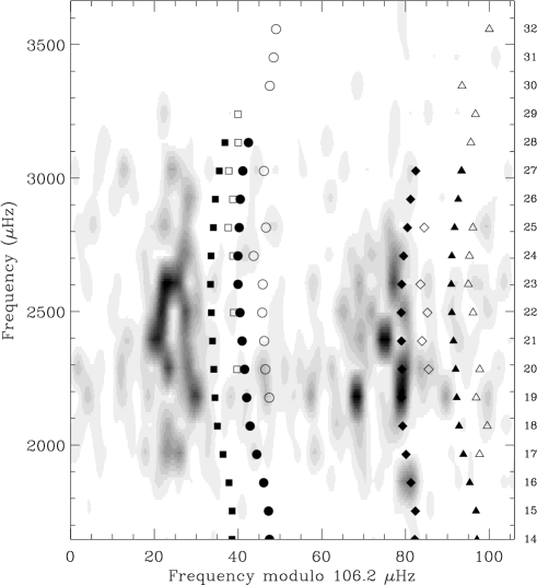
Method 1 is shown in Figure 1 for three main-sequence stars: $\alpha$ Cen A ($\mbox{$\Delta\nu$}\approx 106\,\mbox{$\mu$Hz}$), the Sun ($\mbox{$\Delta\nu$}\approx 135\,\mbox{$\mu$Hz}$) and $\alpha$ Cen B ($\mbox{$\Delta\nu$}\approx 162\,\mbox{$\mu$Hz}$). The greyscale is the power spectrum of $\alpha$ Cen A as observed in a two-site campaign with UVES and UCLES (Bedding et al. 2004), but with weights optimized to minimize the sidelobes (Arentoft et al. 2010). The filled symbols are oscillation frequencies for the Sun (Broomhall et al. 2009; Table 2) after multiplying by 0.7816, and open symbols are frequencies for $\alpha$ Cen B (Kjeldsen et al. 2005) after multiplying by 0.6555. The scaling factors were tuned (using simple ‘trial and error’) to make the ridges for all three stars parallel. Note that scatter of observations about the smooth ridges for $\alpha$ Cen A and B is due to the relatively short duration of the observations (only a few times longer than the mode lifetimes).

There is a systematic progression in stellar parameters (mass, effective temperature and luminosity) as we go from $\alpha$ Cen A through the Sun to $\alpha$ Cen B. We see in Fig. 1 a corresponding progression in the positions of the ridges, which corresponds to a change in $\epsilon$ (see Equation 3). Apart from this, there is a close similarity between the three stars, although there are subtle differences in the curvatures of the ridges and in the small separations between them.

Figure 2: Scaled échelle diagram comparing two simliar stars low-mass stars. Filled symbols: frequencies (unscaled) for $\tau$ Cet. Open symbols: frequencies for $\alpha$ Cen B multiplied by 1.0478. The scaling factor was tuned to make the ridges coincide (Method 1/2). Symbol shapes indicate mode degree: $l=0$ (circles), $l=1$ (triangles), $l=2$ (squares) and $l=3$ (diamonds).

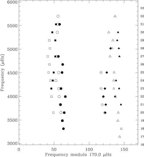
If two stars have very similar parameters, the ridges will almost coincide (Methods 1 and 2 become the same). This is the case for the Sun and the solar twin 18 Sco, recently observed with HARPS and SOPHIE (M. Bazot et al., in prep.), for which the scaling factor gives an extremely precise measurement of the mean density. In this case, we can also use one star as a guide when identifying modes in the other (and eliminating aliases). Another example is shown in Figure 2, for a pair of low-mass stars: the filled symbols show observed frequencies for $\tau$ Cet ($\mbox{$\Delta\nu$}\approx 170\,\mbox{$\mu$Hz}$; Teixeira et al. 2009) and the open filled symbols show those of $\alpha$ Cen B (Kjeldsen et al. 2005) after multiplying by 1.0478.

1 Measuring mean densities

Assuming that a given pair of stars are homologous, (i.e., that Equation 1 holds), the value of the scaling factor gives a direct measurement of their relative densities, without the need to refer to theoretical models. The scaling factors used in Fig. 1 are precise to about 0.05%, in the sense that changing them by this amount produces a noticable deviation from parallelism. If we accept the validity of Equation 1 then our results allow us to measure mean densities for $\alpha$ Cen A and B relative to solar with a precision of 0.1%. We obtain $(0.8601\pm 0.0003)\,\mbox{g\,cm${}^{-3}$}$ for $\alpha$ Cen A and $(2.0018\pm 0.0008)\,\mbox{g\,cm${}^{-3}$}$ for $\alpha$ Cen B. These values agree with those found by comparing the observed frequencie of radial modes with models that have been corrected for the near-surface offset (Kjeldsen et al. 2008; Table 2), but are more precise and do not make any use of model calculations. In practice, however, Equation 1 may not be accurate to this level. In particular, defining a mean density requires that we specify the position of the surface, which is ambiguous, as discussed by Bahcall & Ulrich (1988) in the context of helioseismology. In any case, we have certainly derived mean densities for these stars that are precise enough for any practical application.

The two stars shown in Figure 2, $\tau$ Cet and $\alpha$ Cen B, are even closer. Once again, we found that changing the scaling factor by about 0.05% produced a noticable departure from parallelism. Using the mean density found above for $\alpha$ Cen B, the implied mean density for $\tau$ Cet is $2.198\pm 0.004\,\mbox{g\,cm${}^{-3}$}$, which agrees with the value of $2.21\pm 0.01\,\mbox{g\,cm${}^{-3}$}$ found by Teixeira et al. (2009) but is more precise. Again, we note that being able to measure the homology scaling factor to high precision does not necessarily provide a density measurement with similar accuracy.

2 Ridge identification in F stars

An important application of scaled échelle diagrams is to the problem of ridge identification in F stars. This problem has arisen in the context of several F-type main-sequence stars observed using the CoRoT spacecraft. The first and best-studied example is HD 49933 ($\mbox{$\Delta\nu$}\approx 85\,\mbox{$\mu$Hz}$), whose échelle diagram from 60 days of CoRoT observations showed two broad and very similar ridges (Appourchaux et al. 2008). It was clear that one ridge was due to $l=0$ and $l=2$ modes and the other to $l=1$, but the combination of significant rotational splitting and large linewidths made it difficult to decide which was which. Appourchaux et al. (2008) made a global fit to the line profiles, which led them to favor the possibility they labelled ‘Scenario A’. Further analysis of the same data has been carried out by several groups (Benomar et al. 2009a; Gruberbauer et al. 2009; Roxburgh 2009) and none favored a definite identification, while comparison with theoretical models (Kallinger et al. 2010) gave a better match to Scenario B. Subsequently, the analysis of an additional 180 days of CoRoT observations using revised methods led Benomar et al. (2009b) to reverse the original identification in favor Scenario B.

Two other F stars observed by CoRoT have presented the same problem, namely HD 181906 ($\mbox{$\Delta\nu$}\approx 87.5\,\mbox{$\mu$Hz}$; García et al. 2009) and HD 181420 ($\mbox{$\Delta\nu$}\approx 75\,\mbox{$\mu$Hz}$; Barban et al. 2009). In neither case were the authors able to decide the correct scenario.

Figure 3: Scaled échelle diagrams showing two CoRoT F-type targets that have ambiguous identifications. The filled symbols are oscillation frequencies for HD 49933 from the revised identification (Benomar et al. 2009b; Scenario B). The open symbols are frequencies for HD 181420 (Barban et al. 2009; Scenario 1) after multiplying by 1.144 (upper panel), 1.115 (lower left) and 1.173 (lower right). Symbol shapes indicate mode degree: $l=0$ (circles), $l=1$ (triangles), and $l=2$ (squares).

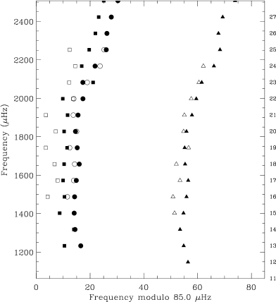
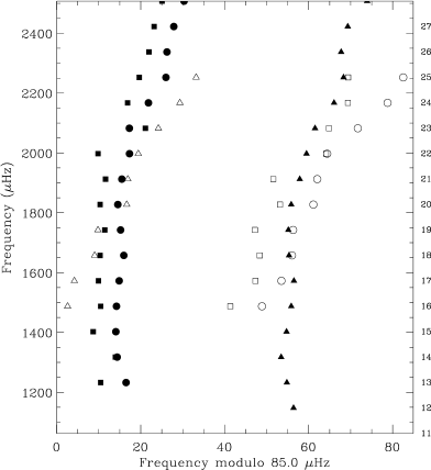
Using scaled échelle diagrams, together with the quite reasonable assumption that $\epsilon$ varies slowly with stellar parameters, we might hope to be able to tie these stars together. Figure 3 shows how this works for two CoRoT targets, HD 49933 and HD 181420. In all three panels, the filled symbols show Scenario B for HD 49933 (Benomar et al. 2009b). The open symbols show Scenario 1 for HD 181420 (Barban et al. 2009) with three different scaling factors. In the upper panel, the scaling factor was chosen to align the ridges as closely as possible, again using trial and error, and we indeed see a good match. However, we should check whether shifting one star by half an order also produces a match. This requires changing the scaling factor by $0.5/n_{\rm max}$, which is about 2.5% in this case. This is shown in the lower two panels of Figure 3, where the scaling factor has been changed in both directions by this amount and then fine-tuned to align the ridges. Neither of these match as well as the upper panel, giving us confidence that Scenario B for HD 49933 is equivalent to Scenario 1 for HD 181420. That is, the two scenarios are either both correct or both wrong.

Figure 4: Scaled échelle diagram comparing HD 49933 with another CoRoT F-type target that has an ambiguous identification. The greyscale is the power spectrum of HD 181906 (García et al. 2009), smoothed to a FWHM of 3 $\mu$Hz. The filled symbols are oscillation frequencies for HD 49933 from the revised identification (Benomar et al. 2009b; Scenario B) after multiplying by 1.011. Symbol shapes indicate mode degree: $l=0$ (circles), $l=1$ (triangles), and $l=2$ (squares).

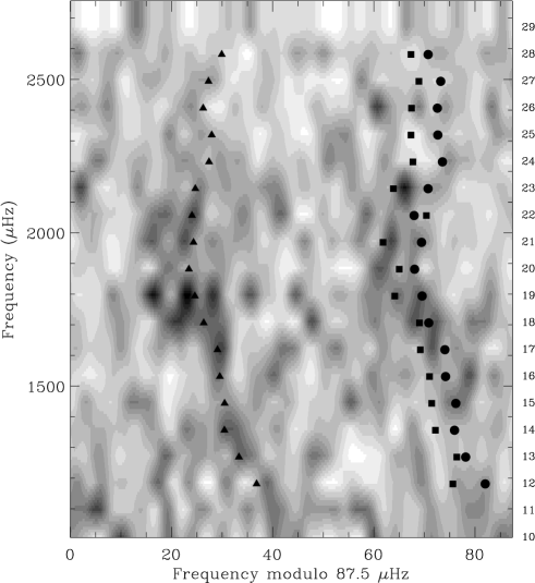
The third problematic CoRoT target mentioned above, which has a significantly lower signal-to-noise ratio, is HD 181906 (García et al. 2009). The power spectrum of this star is shown as the greyscale in Figure 4. Overlaid with filled symbols are the oscillation frequencies for HD 49933 from the revised identification (Benomar et al. 2009b; Scenario B) after multiplying by 1.011. There is good agreement between the stars and, using HD 49933 as a guide, we are able to follow the $l=1$ ridge of HD 181906 down to quite low frequencies. Examining the two possible identifications proposed for HD 181906 by García et al. (2009), we can identify Scenario B for that star with Scenario B for HD 49933. Once again, either both are correct or both are wrong.

Figure 5: Scaled échelle diagram to establish the correct identification for F-type stars. The greyscale is the power spectrum of HD 49385 (Deheuvels et al. 2010), smoothed to a FWHM of 1 $\mu$Hz. The filled symbols are oscillation frequencies for HD 49933 from the revised identification (Benomar et al. 2009b; Scenario B) after multiplying by 0.658. Open symbols are frequencies for $\eta$ Boo (Kjeldsen et al. 2003) after multiplying by 1.390. Symbol shapes indicate mode degree: $l=0$ (circles), $l=1$ (triangles), and $l=2$ (squares).

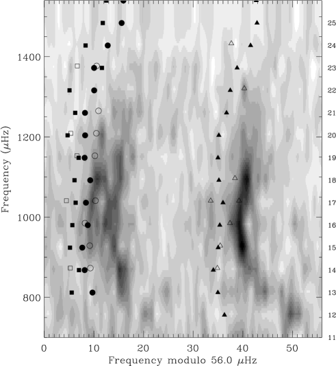
Having linked these three F-type CoRoT targets, all of which have quite similar values of $\Delta\nu$, we would clearly like to confirm the identifications by tying them to other stars whose identifications are secure. We do this in Figure 5. The greyscale shows the power spectrum of the CoRoT target HD 49385 ($\mbox{$\Delta\nu$}\approx 56\,\mbox{$\mu$Hz}$; Deheuvels et al. 2010), for which the $l=0$ and 2 ridges are clearly resolved. The open symbols show frequencies for $\eta$ Boo ($\mbox{$\Delta\nu$}\approx 40\,\mbox{$\mu$Hz}$) after multiplying by 1.390, with mode identifications that were verified by three sets of observations (Kjeldsen et al. 1995, 2003; Carrier et al. 2005) Finally, the filled symbols show once again the revised identification for HD 49933 (Benomar et al. 2009b; Scenario B), this time multiplied by 0.658. These scaling factors differ from unity by more than any others we have considered (since $\Delta\nu$ covers a bigger range). Despite this, we see good alignment of the ridges (Method 1) that gives a consistent picture. Interestingly, HD 49385 shows significantly more curvature at the lowest orders than the other two stars.

To summarise, we conclude that the correct identifications are: Scenario B for HD 49933 (Benomar et al. 2009b), Scenario 1 for HD 181420 (Barban et al. 2009) and Scenario B for HD 181906 (García et al. 2009). The first two of these agree with the conclusions of Mosser & Appourchaux (2009), which were based on autocorrelation analysis of the time series.

4 Conclusions

We have described a method for scaling oscillation frequencies and displaying two or more stars on a single échelle diagram. Assuming that two stars are sufficiently similar to be homologous, the diagram can be used to infer the ratio of their mean densities very precisely, without reference to models. In addition, data from the star with the better signal-to-noise ratio can be used to confirm weaker modes and reject sidelobes in data from a second star. A very important application is to provide a solution to the problem of ridge identification in F-type stars observed by CoRoT, as discussed in Section 2, and we have successfully applied the method to Procyon (Bedding et al. 2010a). Another application is to apply what might be called ensemble asteroseismology to the very large samples of stars being observed by the CoRoT and Kepler space missions. The results of applying this technique to red giants observed with Kepler are described by Bedding et al. (2010b).