Seeing in Color: Jet Superstructure

Abstract

A new class of observables is introduced which aims to characterize the superstructure of an event, that is, features, such as color flow, which are not determined by the jet four-momenta alone. Traditionally, an event is described as having jets which are independent objects; each jet has some energy, size, and possible substructure such as subjets or heavy flavor content. This description discards information connecting the jets to each other, which can be used to determine if the jets came from decay of a color-singlet object, or if they were initiated by quarks or gluons. An example superstructure variable, pull, is presented as a simple handle on color flow. It can be used on an event-by-event basis as a tool for distinguishing previously irreducible backgrounds at the Tevatron and the LHC.

Hadron colliders, such as the LHC at CERN, are fabulous at producing quarks and gluons. At energies well above the confinement scale of QCD, these colored objects are produced in abundance, only hadronizing into color-neutral objects when they are sufficiently far apart. The observed final-state hadrons collimate into jets which, at a first approximation, are in one-to-one correspondence with hard-partons from the short-distance interaction. In fact, this description is so useful that it is usually possible to treat jets as if they are quarks or gluons. Conversely, in a first-pass phenomenological study, it is possible simply to simulate the production of quarks and gluons, assuming they can be accurately reconstructed experimentally from observed jets.

In certain situations, the jet four-momenta alone do not adequately characterize the underlying hard process. For example, when an unstable particle with large transverse momentum decays hadronically, the final state may contain a number of nearly collinear jets. These jets may then be merged by the jet-finder. Or, due to contamination from the underlying event, the energy of the reconstructed jet may not optimally represent the energy of the hard parton, thereby obscuring the short-distance event topology. Over the last few years, a number of improved jet algorithms and filtering techniques have been developed to improve the reconstruction of hard scattering kinematics Butterworth:2008iy ; Kaplan:2008ie ; Ellis:2009me ; Krohn:2009th , with experimentally endorsed successes including reviving a Higgs to $b\bar{b}$ discovery channel at the LHC Butterworth:2008iy (implemented by ATLAS atlas ) and making top-tagging as reliable as $b$-tagging Kaplan:2008ie (implemented by CMS Giurgiu:2009wv ). Nevertheless, there is still a horde of information in the events which these substructure techniques ignore. Jets have color, and are color-connected to each other, providing the event with an observable and characterizable superstructure.

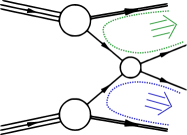
Figure 1: Possible color connections for signal ($pp\to H\to b\bar{b}$) and for background ($pp\to g\to b\bar{b}$).

The term color-connected comes from a graphical picture of the way $SU(3)$ group indices are contracted in QCD amplitudes. To be concrete, consider the production of a Higgs boson at the LHC with the Higgs decaying to bottom quarks. The hard process is $q\bar{q}\to H\to b\bar{b}$. Since the Higgs is a color singlet, the color factor in the leading order matrix element for this production has the form $\mathrm{Tr}[T^{A}T^{B}]\mathrm{Tr}[T^{C}T^{D}]$, where $T^{A}$ are generators of the fundamental representation of $SU(3)$, $A$ and $B$ index the initial state quarks and $C$ and $D$ index the final-state $b$’s. Since $\mathrm{Tr}[T^{C}T^{D}]\propto\delta^{CD}$, the color of $C$ must be the same as $D$, which can be represented graphically as a line connecting quark $C$ to quark $D$. This color string or dipole is shown in Figure 1. An example background process is $q\bar{q}\to g\to b\bar{b}$. Here, there are two possibilities for the color connections: $\mathrm{Tr}[T^{A}T^{C}]\mathrm{Tr}[T^{B}T^{D}]$ and $\mathrm{Tr}[T^{A}T^{D}]\mathrm{Tr}[T^{B}T^{C}]$, both of which connect one incoming quark to one outgoing quark, as shown also in Figure 1. The color string picture treats gluons as bifundamentals, which is correct in the limit of a large the number of colors, $N_{C}\to\infty$. Subleading corrections are included in simulations through color-reconnections, which amount to a $1/N_{C}^{2}\sim 10\%$ effect.

Since color flow is physical, it may be possible to extract the color connections of an event. Such information would be complimentary to the information in the jets’ four-momenta and therefore may help temper otherwise irreducible backgrounds. For example, one application would be in cascade decays from new physics models. In supersymmetry, one often has a large number of jets, originating from on-shell decays like $\tilde{q}\to q\chi$ or from color-singlet gauge boson or gaugino decays. One of the main difficulties in extracting the underlying physics from these decays is the combinatorics: which jets come from which decay? Mapping the superstructure color connections of the events could then greatly enhance our ability to decipher the short-distance physics.

Signal	Background
\psfrag{mpi}[B]{$-\pi$}\psfrag{pi}{$\pi$}\psfrag{eta}{$\mathbf{y}$}\psfrag{phi}{$\boldsymbol{\phi}$}\psfrag{-}[rB]{\scriptsize{$-$}}\psfrag{0}[B]{\scriptsize{$0$}}\psfrag{1}[B]{\scriptsize{$1$}}\psfrag{2}[B]{\scriptsize{$2$}}\psfrag{3}[B]{\scriptsize{$3$}}\includegraphics[height=82.38885pt]{acc_highres3M_dEta1dPhi2_raw_qqHZbb_011_new}	\psfrag{mpi}[B]{$-\pi$}\psfrag{pi}{$\pi$}\psfrag{eta}{$\mathbf{y}$}\psfrag{phi}{$\boldsymbol{\phi}$}\psfrag{-}[rB]{\scriptsize{$-$}}\psfrag{0}[B]{\scriptsize{$0$}}\psfrag{1}[B]{\scriptsize{$1$}}\psfrag{2}[B]{\scriptsize{$2$}}\psfrag{3}[B]{\scriptsize{$3$}}\includegraphics[height=82.38885pt]{acc_highres3M_dEta1dPhi2_raw_qqZbb_011_new}

Figure 2: Accumulated $p_{T}$ after showering a particular partonic phase space point 3 million times. Left has the $b$ and $\bar{b}$ color-connected to each other (signal) and right has the $b$ and $\bar{b}$ color-connected to the beams (background). Contours represent factors of 2 increase in radiation.

In order to extract the color connections, they must persist into the distribution of the observable hadrons. The basic intuition for how the color flow might show up follows from approximations used in parton showers Sjostrand:2006za ; Skands:2009tb . In these simulations, the color dipoles are allowed to radiate through Markovian evolution from the large energy scales associated with the hard interaction to the lower energy scale associated with confinement. These emissions transpire in the rest frame of the dipole. When boosting back to the lab frame, the radiation appears dominantly within an angular region spanned by the dipole, as indicated by the arrows in Figure 1. Alternatively, an angular ordering can be enforced on the radiation (as in herwig Bahr:2008pv ). The parton shower treatment of radiation attempts to include a number of features which are physical but hard to calculate analytically, such as overall momentum and probability conservation or coherence phenomena associated with soft radiation.

It is more important that these effects exist in data than that they are included in the simulation. In fact, color coherence effects have already been seen by various experiments. In $e^{+}e^{-}$ collisions, for example, evidence for color connections between final-state quark and gluon jets was observed in three jet events by JADE at DESY Bartel:1983ii . Later, at LEP, the L3 and DELPHI experiments found evidence for color coherence among the hadronic decay products of color-singlet objects in $W^{+}W^{-}$ events Achard:2003pe ; Abdallah:2006uq . Also, in $p\bar{p}$ collisions at the Tevatron, color connections of a jet to beam remnants have been observed by D0 in $W$+jet events Abbott:1999cu . All of these studies used analysis techniques which were very dependent on the particular event topology. What we will now show is that it is possible to come up with a very general discriminant which can help determine the color flow of practically any event. Such a tool has the potential for wide applicability in new physics searches at the LHC.

Signal Pull	Background Pull
\psfrag{th}{$\boldsymbol{\theta_{t}}$}\psfrag{mp}{$\boldsymbol{\left|\vec{t}\right|}$}\psfrag{mpi}{$-\pi$}\psfrag{pi}{$\pi$}\psfrag{0.04}{\scriptsize{$0.04$}}\psfrag{0.02}{\scriptsize{$0.02$}}\psfrag{0}{\scriptsize{$0$}}\includegraphics[height=91.0598pt]{pull_2d_signal}	\psfrag{th}{$\boldsymbol{\theta_{t}}$}\psfrag{mp}{$\boldsymbol{\left|\vec{t}\right|}$}\psfrag{mpi}{$-\pi$}\psfrag{pi}{$\pi$}\psfrag{0.04}{\scriptsize{$0.04$}}\psfrag{0.02}{\scriptsize{$0.02$}}\psfrag{0}{\scriptsize{$0$}}\includegraphics[height=91.0598pt]{pull_2d_background}

Figure 3: Event-by-event density plot of the pull vector of the $b$ jet in polar coordinates. The signal (connected to $\bar{b}$ jet) is on the left, the background (connected to the left-going, $y=-\infty$ beam) is on the right. $10^{5}$ events are shown.

For an example, we will use Higgs production in association with a $Z$. The $Z$ allows the Higgs to have some $p_{T}$ so that its $b\bar{b}$ decay products are not back-to-back in azimuthal angle, $\phi$. Our benchmark calculator will be madgraph Alwall:2007st for the matrix elements interfaced to pythia 8 Sjostrand:2007gs for the parton shower, hadronization and underlying event, with other simulations used for validation.

To begin, we isolate the effect of the color connections by fixing the parton momentum. We compare events with $Zb\bar{b}$ in the final state (with $Z\to$ leptons) in which the quarks are color-connected to each other (signal) versus color-connected to the beam (background). In Figure 2, we show the distribution of radiation for a typical case, where $(y,\phi)=(-0.5,-1)$ for one $b$ and $(y,\phi)=(0.5,1)$ for the other, with $p_{T}=200$ GeV for each $b$, where $y$ is the rapidity. For this figure, we have showered and hadronized the same parton-level configuration over and over again, accumulating the $p_{T}$ of the final-state hadrons in $0.1\times 0.1$ bins in $y$-$\phi$ space. The color connections are unmistakable.

The superstructure feature of the jets in Figure 2 that we want to isolate is that the radiation in each signal jet tends to shower in the direction of the other jet, while in the background it showers mostly toward the beam. In other words, the radiation on each end of a color dipole is being pulled towards the other end of the dipole. This should therefore show up in a dipole-type moment constructed from the radiation in or around the individual jets. For dijet events, like those shown in Figure 2, one could imagine constructing a global event shape from which the moment could be extracted. However, a local observable, constructed only out of particles within the jet, has a number of immediate advantages. For one, it will be a more general-purpose tool, applying to events with any number of jets. It should also be easier to calibrate on data, since jets are generally better understood experimentally than global event topologies. Therefore, as a first attempt at a useful superstructure variable, we construct an observable out of only the particles within the jets themselves.

In constructing a jet moment, there are a number of ways to weight the momentum, such as by energy or $p_{T}$, and to define the center the jet. These are all basically the same, but we have found that the most effective combination is a $p_{T}$-weighted vector, which we call pull, defined by

$$\vec{t}=\sum_{i\in\text{jet}}\frac{p_{T}^{i}\,|r_{i}|}{p_{T}^{\text{jet}}}\,\vec{r}_{i}\,.$$ (1)

Here, $\vec{r}_{i}=(\Delta y_{i},\Delta\phi_{i})=\vec{c}_{i}-\vec{J}$, where $\vec{J}=(y_{J},\phi_{J})$ is the location of the jet and $\vec{c}_{i}$ is the position of a cell or particle with transverse momentum $p_{T}^{i}$. Note that we use rapidity $y_{J}$ for the jet instead of pseudorapidity ($\eta_{J}$); because the jet is massive this makes $\vec{r}_{i}$ boost invariant and a better discriminant (rapidity and pseudorapidity are equivalent for the effectively massless cells/particles, $\vec{c}_{i}$). The centroid (Eq. (1) without the $|r_{i}|$ factor) is usually almost identical to $\vec{J}$, the location of the jet four-vector in the $E$-scheme (the sum of four-momenta of the jet constituents).

An important feature of the pull vector $\vec{t}$ is that it is infrared safe. If a very soft particle is added to the jet, it has negligible $p_{T}$, and therefore a negligible effect on $\vec{t}$. Moreover, since pull is linear in $p_{T}$, if a particle splits into two collinear particles at the same $\vec{r}$, the pull vector is also unchanged. This property guarantees that pull should be fairly insensitive to fine details of the implementation, such as the spatial granularity or energy resolution of the calorimeters.

\psfrag{th}{$\boldsymbol{\theta_{t}}$}\psfrag{signal}{ signal}\psfrag{background}{ \color[rgb]{0.0,0.0,0.5}background}\psfrag{towardOtherJet}{ toward other jet}\psfrag{PYTHIA6}{ {\sc pythia}6}\psfrag{PYTHIA8}{ {\sc pythia}8}\psfrag{HERWIGpp}{ {\sc herwig}++}\psfrag{mpi}{$-\pi$}\psfrag{pi}{$\pi$}\psfrag{0}{$0$}\psfrag{1}{$1$}\psfrag{2}{$2$}\psfrag{3}{$3$}\includegraphics[width=162.6075pt]{generators}

Figure 4: Distribution of the pull angle (for the $b$ jet) with $\Delta y_{b\bar{b}}=1$ and $\Delta\phi_{b\bar{b}}=2$, for signal and background, showered $10^{5}$ times with different Monte Carlos.

The event-by-event distribution of the pull for the left $b$ jet from Figure 2 is shown in Figure 3 in polar coordinates, $\vec{t}=(|\vec{t}|\cos\theta_{t},|\vec{t}|\sin\theta_{t})$, where $\theta_{t}=0$ points towards the right-going beam, $\theta_{t}=\pm\pi$ points towards the left-going beam, and $\theta_{t}\approx 0.7$ toward the other $b$ jet. This figure shows density plots of the $\vec{t}$ distributions on an event-by-event basis for the signal and background cases for this particular fixed parton-level phase space point. For this figure, we use as input the four-momenta of all long-lived observable particles. If instead, we use the hadronic energy in $0.1\times 0.1$ cells treated as massless four-vectors, the distribution of pull vectors is nearly identical.

We can see that most of the discriminating information is in the pull angle, $\theta_{t}$, rather than the magnitude $|\vec{t}|$. This leads to Figure 4, which shows the distribution of the pull angle for the signal and the background in this particular kinematic configuration. This figure also shows that the pull vector is not particularly sensitive to the Monte Carlo program used to generate the sample; the pull angle distributions for herwig++ 2.4.2 Bahr:2008pv , pythia 8.130 Sjostrand:2007gs , and pythia 6.420 with the $p_{T}$-ordered shower Sjostrand:2006za are all quite similar.

The previous three figures all have the parton momentum fixed. Similar distributions result from other phase space points. We fixed the parton momentum to show the usefulness of pull in situations which would be indistinguishable using the jet four-momenta alone. This exercise controls for correlations between pull and matrix-element-level kinematic discriminants. Also, note that there is another possible color-flow for the background events, where the left-going jet is color-connected to the right-going beam. Then, the most-likely pull angle would be more similar to the signal. Fortunately, this only occurs about 10% of the time for the dominant background.

Pull of Higher $\mathbf{p_{T}}$ $\mathbf{b}$	Pull of Lower $\mathbf{p_{T}}$ $\mathbf{b}$
\psfrag{th}[l]{$\boldsymbol{\Delta\theta_{t}}$}\psfrag{signal}[l]{ signal}\psfrag{background}[l]{\color[rgb]{0.0,0.0,0.5}background}\psfrag{mpi}[l]{$-\pi$}\psfrag{pi}[l]{$\pi$}\psfrag{0}[l]{$0$}\psfrag{1}[l]{$1$}\psfrag{2}[l]{$2$}\psfrag{3}[l]{$3$}\includegraphics[width=97.56383pt]{pull_toward_otherjet_high_pt}	\psfrag{th}[l]{$\boldsymbol{\Delta\theta_{t}}$}\psfrag{signal}[l]{ signal}\psfrag{background}[l]{\color[rgb]{0.0,0.0,0.5}background}\psfrag{mpi}[l]{$-\pi$}\psfrag{pi}[l]{$\pi$}\psfrag{0}[l]{$0$}\psfrag{1}[l]{$1$}\psfrag{2}[l]{$2$}\psfrag{3}[l]{$3$}\includegraphics[width=97.56383pt]{pull_toward_otherjet_low_pt}

Figure 5: Pull angles in the $b$ or $\bar{b}$ jet in $HZ\to Zb\bar{b}$ signal events and their $Z+b\bar{b}$ backgrounds. For each event, $\Delta\theta_{t}=0$ is defined to point toward the other $b$ jet. $3\times 10^{5}$ events are shown.

The next step is to see if pull is useful given the full distribution of signal and background events at the LHC. The pull angle for the full $ZH\to Zb\bar{b}$ signal and $Zb\bar{b}$ backgrounds still presents a strong discriminant, as can be seen in Figure 5. Here, we have performed a full simulation with madgraph 4.4.26 Alwall:2007st and pythia 8.130 Sjostrand:2007gs , including underlying event and hadronization. We choose a parton-level cut of $p_{T}>15$ GeV for the $b$ quarks, find the jets with the anti-$k_{T}$ algorithm with $R=0.7$, require the reconstructed mass to be within a 20 GeV window around the Higgs mass (120 GeV), and construct the pull angle on the radiation within each jet.

Next, let us consider some other possibilities. It is natural to look at higher moments, such as those contained in the covariance tensor

$${\mathbf{C}}=\sum_{i\in\text{jet}}\frac{p_{T}^{i}|r_{i}|}{p_{T}^{\text{jet}}}\left(\begin{array}[]{cc}\Delta y_{i}^{2}&\Delta y_{i}\,\Delta\phi_{i}\\ \Delta\phi_{i}\,\Delta y_{i}&\Delta\phi_{i}^{2}\end{array}\right)\,.$$ (2)

The eigenvalues $a\geq b$ of this tensor are similar to the semimajor and semiminor axes of an elliptical jet. The overall size of these $g=\sqrt{a^{2}+b^{2}}$ provides a decent characterization of whether the jet is initiated by a quark or gluon. Gluon jets, since they cap two color dipoles, generally have more radiation and lead to jets with larger values of $g$. However, $g$ is strongly correlated with the mass of a jet and the mass-to-$p_{T}$ ratio. Since mass and $p_{T}$ are contained in the jet four-momentum, this measure of size is not likely to provide a new handle for irreducible backgrounds. Other combinations of second-moment eigenvalues, such as the eccentricity $e=\sqrt{(a^{2}-b^{2})/a}$ or orientation of the ellipse, seem much less useful. While one might expect gluon jets to be fairly elliptical, due to their being pulled in two directions, in fact quarks turn out to be equally elliptical; we have not found a significant difference in the eccentricity of quark and gluon jets. Going to third or higher moments is straightforward, but serves no immediate purpose.

We conclude that the pull angle is the most useful moment-type observable for determining the color superstructure of an event. Besides moments, one could attempt to use more global observables, such as the amount of radiation around or between jets. As we have mentioned, such an approach is in principle promising, but the analysis would have to be very process-dependent. A nice feature of pull is its universality. Although we have used as a canonical example Higgs production in association with a $Z$ boson, the pull angle can be used to characterize any process with jets, such as cascade decays in supersymmetry or resonance decays in composite models. In fact, for practically any new physics scenario involving jets, finding the color connections would be very helpful, and the pull angle provides a simple tool to extract this information.

In order to apply superstructure variables to new physics searches, it will be critical to first validate them on standard model data. One useful class of events is $t\bar{t}$ production. For semileptonic $t\bar{t}$ decays, we can get an arbitrarily clean sample by tightening the $b$-tags, top mass window, and leptonic $W$ reconstruction. This will give us a pure sample of hadronic, boosted $W$ bosons. The two light quark jets from the $W$ decay should be color-connected, and the pull angle of each quark can be measured on data. The same sample also provides $b$ jets connected to the beam. We have tested this idea in simulations of $t\bar{t}$ events, and have found that the pull angle distribution in the hadronic $W$ decay products is in fact similar to that of the the Higgs decay in Figure 5.

Finally, let us mention a few words about the choice of jet algorithm. Using the program fastjet v2.4 Cacciari:2005hq for jet finding, we found that the anti-$k_{T}$Cacciari:2008gp algorithm, which takes radiation from more circular regions, gives better results than $k_{T}$ Catani:1993hr , SIScone Salam:2007xv , or Cambridge/Aachen Dokshitzer:1997in . It is also possible to find the jets with one algorithm and size, say $R=0.7$ and then use a larger size, say $R=1.2$, to calculate the moment. We have not found an obvious improvement from doing this, but such possibilities should be explored. For example, if the pull angle were to be used by an experimental collaboration in Higgs search, a few percent improvement could probably be gained by optimizing the algorithm in coordination with the detailed experimental parameters. It would also be worth investigating whether jet filtering Butterworth:2008iy or trimming Krohn:2009th , could help make pull or other superstructure variables even more discriminating. Although there is still a lot of room for improvement, it is clear that color flows and jet superstructure can be useful observables at hadron colliders, and are worth understanding better.

The authors would like to thank David E. Kaplan, David Krohn, Steve Mrenna, Michael Peskin and Keith Rehermann for useful discussions and the Jet Substructure Workshop at the University of Washington, the FAS Research Computing Group at Harvard University and the Department of Energy, under Grant DE-AC02-76CH03000, for support.

References

- (1) J. M. Butterworth, A. R. Davison, M. Rubin and G. P. Salam, Phys. Rev. Lett. 100, 242001 (2008) [arXiv:0802.2470 [hep-ph]].
- (2) D. E. Kaplan, K. Rehermann, M. D. Schwartz and B. Tweedie, Phys. Rev. Lett. 101, 142001 (2008) [arXiv:0806.0848 [hep-ph]].
- (3) S. D. Ellis, C. K. Vermilion and J. R. Walsh, arXiv:0912.0033 [hep-ph].
- (4) D. Krohn, J. Thaler and L. T. Wang, arXiv:0912.1342 [hep-ph].
- (5) ATL-PHYS-PUB-2009-088. ATL-COM-PHYS-2009-345.
- (6) G. Giurgiu [for the CMS collaboration], arXiv:0909.4894
- (7) T. Sjostrand, S. Mrenna and P. Z. Skands, JHEP 0605, 026 (2006)
- (8) P. Z. Skands and S. Weinzierl, Phys. Rev. D 79, 074021 (2009)
- (9) M. Bahr et al., Eur. Phys. J. C 58, 639 (2008)
- (10) W. Bartel et al. [JADE Collaboration], Z. Phys. C 21, 37 (1983).
- (11) P. Achard et al. [L3 Collaboration], Phys. Lett. B 561, 202 (2003)
- (12) J. Abdallah et al. [DELPHI Collaboration], Eur. Phys. J. C 51, 249 (2007)
- (13) B. Abbott et al. [D0 Collaboration], Phys. Lett. B 464, 145 (1999)
- (14) J. Alwall et al., JHEP 0709, 028 (2007)
- (15) T. Sjostrand, S. Mrenna and P. Z. Skands, Comput. Phys. Commun. 178, 852 (2008)
- (16) M. Cacciari and G. P. Salam, Phys. Lett. B 641, 57 (2006)
- (17) M. Cacciari, G. P. Salam and G. Soyez, JHEP 0804, 063 (2008) [arXiv:0802.1189 [hep-ph]].
- (18) S. Catani, Y. L. Dokshitzer, M. H. Seymour and B. R. Webber, Nucl. Phys. B 406, 187 (1993).
- (19) G. P. Salam and G. Soyez, JHEP 0705, 086 (2007)
- (20) Y. L. Dokshitzer, G. D. Leder, S. Moretti and B. R. Webber, JHEP 9708, 001 (1997)