Abstract

We report on the computation of the critical point of the deconfinement phase transition, critical indices and the string tension in the compact three dimensional $U(1)$ lattice gauge theory at finite temperatures. The critical indices govern the behavior across the deconfinement phase transition in the pure gauge $U(1)$ model and are generally expected to coincide with the critical indices of the two-dimensional $XY$ model. We studied numerically the $U(1)$ model for $N_{t}=8$ on lattices with spatial extension ranging from $L=32$ to $L=256$. Our determination of the infinite volume critical point on the lattice with $N_{t}=8$ differs substantially from the pseudo-critical coupling at $L=32$, found earlier in the literature and implicitly assumed as the onset value of the deconfined phase. The critical index $\nu$ computed from the scaling of the pseudo-critical couplings with the extension of the spatial lattice agrees well with the $XY$ value $\nu=1/2$. On the other hand, the index $\eta$ shows large deviation from the expected universal value. The possible reasons of such behavior are discussed in details.

  e-mail addresses:

^∗oleg@bitp.kiev.ua, ^∗∗fiore,papa@cs.infn.it, ^∗∗∗Mario.Gravina@th.u-psud.fr

1 Introduction

In this article we continue our exploration of the deconfinement phase transition in the three-dimensional ($3d$) $U(1)$ lattice gauge theory (LGT) started in Ref. [1]. The partition function of the compact version of this model can be written as

$$Z(\beta_{t},\beta_{s})=\int_{0}^{2\pi}\prod_{x\in\Lambda}\>\prod_{n=0}^{2}\frac{d\omega_{n}(x)}{2\pi}\ \exp{S[\omega]}\ ,$$ (1)

where $\Lambda$ is an $L^{2}\times N_{t}$ lattice, $S$ is the Wilson action

$$S[\omega]=\beta_{s}\sum_{p_{s}}\cos\omega(p_{s})+\beta_{t}\sum_{p_{t}}\cos\omega(p_{t})$$ (2)

and sums run over all space-like ($p_{s}$) and time-like ($p_{t}$) plaquettes. The plaquette angles $\omega(p)$ are defined in the standard way. The anisotropic couplings $\beta_{t}$ and $\beta_{s}$ are defined in Ref. [1]. Since we study the theory at finite temperature, periodic boundary conditions in the temporal direction are imposed on the gauge fields.

Let us recapitulate briefly what is known and/or expected about the critical behavior of the $3d$ $U(1)$ LGT at finite temperature. At zero temperature the theory is confining at all values of the bare coupling constant [2], while at finite temperature the theory undergoes a deconfinement phase transition. It is well known that the partition function of the $3d$ $U(1)$ LGT in the Villain formulation coincides with that of the $2d$ $XY$ model in the leading order of the high-temperature expansion [3]. When combined with the universality conjecture by Svetitsky-Yaffe [4], this result makes one to conclude that the deconfinement phase transition belongs to the universality class of the $2d$ $XY$ model, which is known to have Berezinskii-Kosterlitz-Thouless (BKT) phase transition of infinite order [5, 6]. It is therefore generally expected the critical behavior of the $3d$ $U(1)$ LGT to coincide with that of the $XY$ model. In particular, one might expect the critical behavior of the Polyakov loop correlation function $\Gamma(R)$ to be governed by the following expressions

$$\Gamma(R)\ \asymp\ \frac{1}{R^{\eta(T)}}\ ,$$ (3)

for $\beta\geq\beta_{c}$ and

$$\Gamma(R)\ \asymp\ \exp\left[-R/\xi(t)\right]\ ,$$ (4)

for $\beta<\beta_{c}$, $t=\beta_{c}/\beta-1$. Here, $R\gg 1$ is the distance between test charges, $T$ is the temperature and $\xi\sim e^{bt^{-\nu}}$ is the correlation length. Such behavior of $\xi$ defines the so-called essential scaling. The critical indices $\eta(T)$ and $\nu$ are known from the renormalization-group (RG) analysis of the $XY$ model: $\eta(T_{c})=1/4$ and $\nu=1/2$, where $T_{c}$ is the BKT critical point. Therefore, the critical indices $\eta$ and $\nu$ should be the same in the finite-temperature $U(1)$ model if the Svetitsky-Yaffe conjecture holds in this case.

The renormalization-group calculations of the RG flow, presented in Ref. [4], gave support to the BKT scaling scenario. However, the critical indices have not been computed. The direct numerical check of these predictions was performed on lattices $L^{2}\times N_{t}$ with $L=16,32$ and $N_{t}=4,6,8$ in Ref. [7]. Though the authors of Ref. [7] confirm the expected BKT nature of the phase transition, the reported critical index is almost three times that predicted for the $XY$ model, $\eta(T_{c})\approx 0.78$. More recent numerical simulations of Ref. [8] have been mostly concentrated on the study of the properties of the high-temperature phase. What is important for us here is the derivation of the critical point in Refs. [7, 8]. In these papers it was found that, for the isotropic lattice $\beta_{s}=\beta_{t}=\beta$ with $L=32$ and $N_{t}=8$, the pseudo-critical point is $\beta_{pc}=2.30(2)$ for Ref. [7] and $\beta_{c}\approx 2.346(2)$ for Ref. [8]. Values of $\beta$ above these values were taken implicitly as belonging to the deconfined phase. We shall comment on this derivation later since our result for the infinite volume critical coupling differs essentially for this choice of $N_{t}$.

In our previous paper [1] we have studied the model on extremely anisotropic lattice with $\beta_{s}=0$. In this limit the model exhibits the deconfinement phase transition which gives the possibility to study the critical behavior. We presented simple analytical consideration which showed that in the limits of both small and large $\beta_{t}$ such anisotropic model reduces to the $2d$ $XY$ model with some effective couplings. Then we performed numerical simulations of the effective spin model for the Polyakov loop which can be exactly computed in the limit $\beta_{s}=0$. We used lattices with $N_{t}=1,4,8$ and with the spatial extent $L\in[64,256]$. Our main goal was to determine the critical index $\eta$ supposing that the scaling known from the study of the $XY$ model holds also in our case. The main conclusion of our investigation was that the value of the index $\eta$ is well compatible with the $XY$ value. We may thus assume that at least in the limit $\beta_{s}=0$ the $3d$ $U(1)$ LGT does belong to the universality class of the $XY$ model.

Encouraged by these findings we have decided to simulate directly the isotropic model on the lattice with $N_{t}=8$. In this paper we present the results of these simulations for a number of different quantities. Our general strategy is essentially the same as in the previous paper. Namely, we postulate that the scaling laws of the $XY$ model can be used to study the critical behavior of the gauge model. We believe that the information gathered so far allows for such an approach to be trustworthy. Nevertheless, in doing so we have encountered certain surprises. First of all, the infinite volume critical coupling turned out to be essentially higher than the values for the pseudo-critical couplings reported in Refs. [7, 8]. As a consequence, the values of $\beta$ used in Ref. [8] to study the deconfinement phase lie well inside the confinement phase when the thermodynamic limit is considered. Secondly, the index $\nu$ extracted from the scaling of the pseudo-critical couplings with $L$ does agree well with the expected $XY$ value $\nu=1/2$. However, the index $\eta$ was found to be strikingly different from the $XY$ value, namely $\eta\approx 0.50$. While the value $\eta\approx 0.78$ obtained in Ref. [7] could, in principle be attributed to rather small lattices used, $L=32$, and to an incorrect location of the critical point, our result is almost insensitive to varying the spatial extent if $L$ is large enough.

This paper is organized as follows. In the next section we describe briefly our numerical procedure. The result of simulations are presented in the Section 3. Conclusions and discussion are given in the Section 4.

2 Numerical set-up

With the aim of calculating the critical indices and then identifying the universality class of the $3d$ $U(1)$ LGT, we simulated the system on lattices of the type $L^{2}\times N_{t}$, with $N_{t}=8$ fixed and $L$ increasing towards the thermodynamic limit. In the adopted Monte Carlo algorithm a sweep consisted in a mixture of one Metropolis update and five microcanonical steps. Measurements were taken every 10 sweeps in order to reduce the autocorrelation and the typical statistics per run was about 100k. The error analysis was performed by the jackknife method over bins at different blocking levels.

The observable used as a probe of the two phases of the finite temperature $3d$ $U(1)$ LGT is the Polyakov loop, defined as

$$P(\vec{x})=\prod_{t}U_{0}(\vec{x},t)\quad,$$ (5)

where $U_{0}(\vec{x},t)$ is the temporal link attached at the spatial point $\vec{x}$. The effective theory for the Polyakov loop is two-dimensional and possesses global $U(1)$ symmetry. Since the global symmetry cannot be broken spontaneously in two dimensions owing to the Mermin-Wagner-Coleman theorem the expectation value of the Polyakov loop vanishes in the thermodynamic limit. On a finite lattice $\langle\sum_{\vec{x}}P(\vec{x})\rangle=0$ due to $U(1)$ symmetry (if the boundary conditions used preserve the symmetry). This is confirmed by the numerical analysis on the periodic lattice: in the confined (small $\beta$) phase the values taken by the Polyakov loop in a typical Monte Carlo ensemble scatter around the origin of the complex plane forming a uniform cloud, whereas in the deconfined (high $\beta$) phase they distribute on a ring, the thermal average being equal to zero in both cases (see Fig. 1 for an example of this behavior in the case $L=32$, where the transition occurs at $\beta$=2.346(2), according to Ref. [8]). What really feels the transition is then the absolute value of $P$, which has been chosen to be the order parameter in this work. It is worth to stress that this kind of dynamics is the same presented by the spin magnetization in the $2d$ $XY$ model.

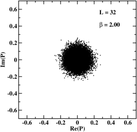
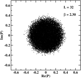
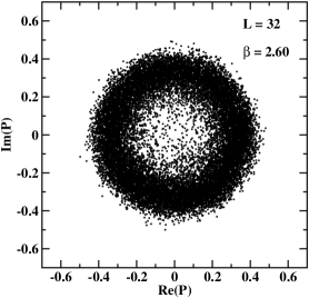
Figure 1: Scatter plot of the Polyakov loop for $\beta=2.00,2.30,2.60$ on the $32^{2}\times 8$ lattice.

3 Results at $\beta_{s}=\beta_{t}$

At finite volume the transition manifests through a peak in the magnetic susceptibility of the Polyakov loop, defined as

$$\chi_{L}=L^{2}(\langle|P|^{2}\rangle-\langle|P|\rangle^{2})\quad,\quad P=\frac{1}{L^{2}}\ \sum_{x}P(\vec{x})\quad.$$ (6)

The value of the coupling at which this happens is the pseudo-critical coupling, $\beta_{pc}$. By increasing the spatial volume, the position of the peak moves towards the (nonuniversal) infinite volume critical coupling, $\beta_{c}$. In Fig. 2 the behavior of $\chi_{L}$ around the transition is shown for $L=48,64,128$. The value of $\beta_{pc}$ for a given $L$ is determined by interpolating the values of the susceptibility $\chi_{L}$ around the peak by a Lorentzian function. In Table 1 we summarize the resulting values of $\beta_{pc}$ and the peak values of the susceptibility $\chi_{L}$ for the several volumes considered in this work (we included also the determination for $L=32$, taken from the first paper in Ref. [8]).

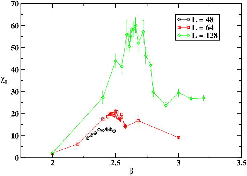
Figure 2: Polyakov loop susceptibility $\chi_{L}$ on the lattices $L^{2}\times 8$, with $L=48,64,128$.

Table 1: $\beta_{pc}$ and peak value of the Polyakov loop susceptibility $\chi_{L}$ on the lattices $L^{2}\times 8$.

$L$	$\beta_{pc}$	$\chi_{L,\mbox{\scriptsize max}}$
32	2.346(2), Ref. [8]
48	2.4238(67)	12.93(41)
64	2.4719(39)	20.09(66)
96	2.5648(96)	38.8(1.6)
128	2.6526(59)	60.1(3.5)
150	2.68(1)	92.6(8.0)
200	2.7336(69)	144(12)
256	2.7780(40)	220(20)

In order to apply the finite size scaling (FSS) program, the location of the infinite volume critical coupling $\beta_{c}$ is needed. The scaling law by which $\beta_{c}$ can be extracted from the known values of $\beta_{pc}(L)$ depends on the nature of the transition and, in particular, on the behavior of the correlation length. There are, in principle, two hypotheses to be tested: first order and BKT transition. The hypothesis of first order transition is not incompatible with data for the peak susceptibility for $L\geq 128$. However, the corresponding scaling law for the pseudo-critical couplings,

$$\beta_{pc}=\beta_{c}+\frac{A}{L^{2}}\quad,$$ (7)

seems to be ruled out by our data ($\chi^{2}$/d.o.f equal to 5.6 for $L\geq 96$, 3.7 for $L\geq 128$, 2.1 for $L\geq 96$).

Assuming the essential scaling of the BKT transition, i.e. $\xi\sim e^{bt^{-\nu}}$, the scaling law for $\beta_{pc}$ becomes

$$\beta_{pc}=\beta_{c}+\frac{A}{(\ln L+B)^{\frac{1}{\nu}}}\quad.$$ (8)

The index $\nu$ characterizes the universality class of the system. For example, $\nu=1/2$ holds for the 2$d$ $XY$ universality class.

We tried at first a 4-parameter fit of the data for $\beta_{pc}(L)$ given in Table 1 with the law given in Eq. (8). We excluded systematically from the fit the data for $\beta_{pc}(L)$ at the lowest spatial volumes, looking for a region of stability of the parameters. Defining $L_{\mbox{\scriptsize min}}$ as the smallest value of $L$ for which $\beta_{pc}(L)$ has been considered in the fit, we could not find a stable fit for $L_{\mbox{\scriptsize min}}<96$. In particular, we found that the $\chi^{2}$/d.o.f. is $\approx 10$ for $L_{\mbox{\scriptsize min}}=32$, $\approx 6$ for $L_{\mbox{\scriptsize min}}=48$ and $\approx 1.8$ for $L_{\mbox{\scriptsize min}}=64$. Moreover, we observed a strong dependence of the fit parameters on the starting values used in the MINUIT minimization code, although the resulting fitting curve turned out to be in general rather stable. The instability of parameters becomes less severe when $L_{\mbox{\scriptsize min}}$ increases and, in particular, for $L_{\mbox{\scriptsize min}}=64$ the parameter $\nu$ becomes compatible with the $XY$ value, $\nu=0.5$, although still undergoing large fluctuations under change of the starting conditions of the MINUIT minimization procedure. A stable fit could be achieved only for $L_{\mbox{\scriptsize min}}=96$ and these are the resulting parameters:

$$\beta_{c}=3.06(16)\;,\;\;\;\;\;A=-5.3(5.1)\;\;\;\;\;\;B=-1.4(1.0)\;,\;\;\;\;\;\nu=0.49(16)\;\;\;\;\;(\chi^{2}/\mbox{d.o.f.}=1.5).$$

We repeated then the fit with the law (8) keeping the parameter $\nu$ fixed at the $XY$ value, $\nu=1/2$, thus reducing to three the number of free parameters in the fit. In this case, the fit instability is highly suppressed with respect to the previous 4-parameter analysis and, indeed, already for $L_{\mbox{\scriptsize min}}\geq 48$ we can quote stable values of the fit parameters (see Table 2). One can see that an acceptable $\chi^{2}$/d.o.f. and a stable fit are obtained for $L_{\mbox{\scriptsize min}}=64$ and $L_{\mbox{\scriptsize min}}=96$ and that, for the latter volume, $\beta_{c}$ is consistent with the result of the 4-parameter fit. We take therefore $\beta_{c}=3.06(11)$ as our estimation for the infinite volume critical coupling. The determination of $\beta_{c}$ is the first main result of this work.

While performing this work, we considered also the possibility to extract the index $\nu$ from directly fitting the essential scaling law $\xi\sim e^{bt^{-\nu}}$ against lattice data for the correlation length taken for several $\beta$ values and for several volumes. To be more precise, for each considered value of $L$ and for several $\beta$ values across $\beta_{pc}(L)$, we determined the correlation length $\xi_{L}$ as the inverse decay length of the 2-point correlator of the Polyakov loops, interpolating the latter as if the exponential fall-off with the distance apply even above $\beta_{pc}$, where, in fact, this correlator decays power-like (see Fig. 3). At each volume it happens that $\xi_{L}$ defined in this way increases with $\beta$ till $\beta\approx\beta_{pc}$ and then saturates, consistently with the fact that the region of power-like behavior has been reached. It occurs, however, that the set of all lattice data for the correlation length $\xi_{L}$ that, at each volume, belong to the region $\beta<\beta_{pc}(L)$, lie approximately on the same curve. This is expected to occur more and more accurately as the thermodynamic limit is approached. One could then try to fit the lattice data for $\xi_{L}$ falling on this curve with the essential scaling law and extract $\nu$. Unfortunately, the quality of our data did not allow us to have a stable fit and we had to reject this method. It cannot be excluded, however, that it will be reconsidered in possible future studies of the same kind.

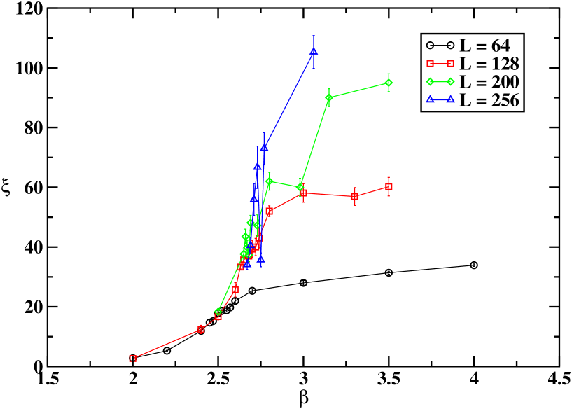
Figure 3: Correlation length vs $\beta$ on the lattices $L^{2}\times 8$, with $L$=64, 128, 200, 256. The correlation length is determined as if the exponential fall-off with distance of the 2-point correlator of the Polyakov loop apply for all $\beta$ values.

Table 2: Results of the 3-parameter fit of the values of $\beta_{pc}(L)$ with the law (8), $\nu=1/2$ fixed.

$L_{\mbox{\scriptsize min}}$	$\beta_{c}$	$A$	$B$	$\chi^{2}$/d.o.f.
32	5.103(50)	-1523(86)	20.03(48)	13.
48	4.65(23)	-699(239)	13.8(2.1)	4.3
64	3.44(15)	-42(24)	2.4(1.4)	1.2
96	3.06(11)	-4.7(4.3)	-1.5(1.1)	0.76

Once an estimation for $\beta_{c}$ has been achieved, we can use the FSS analysis, which holds just at $\beta_{c}$, to extract other critical indices. An interesting example is the magnetic critical index, $\eta$, which enters the scaling law

$$\chi_{L}(\beta_{c})\sim L^{2-\eta}\quad.$$ (9)

Actually in this law one should consider logarithmic corrections (see [9, 10] and references therein) and, indeed, recent works on the $XY$ universality class generally include them. However, taking these corrections into account for extracting critical indices calls for very large lattices even in the $XY$ model; for the theory under consideration to be computationally tractable, we have no choice but to neglect logarithmic corrections.

Setting the coupling $\beta$ at the value of our best estimation for $\beta_{c}$, i.e. $\beta=3.06$, we determined the susceptibilities $\chi_{L}(\beta_{c})$ for several volumes (see Table 3 for the results). Then, following FSS, we fitted the results with the law $\chi_{L}(\beta_{c})=AL^{2-\eta}$ and got

$$A=0.0171(10),\quad\eta=0.496(15)\quad(\chi^{2}/\mbox{d.o.f.}=0.60)\quad.$$ (10)

This is the second main result of our paper. We stress that this value for $\eta$ is by far incompatible with the 2$d$ $XY$ value, $\eta_{XY}=0.25$. The most extreme consequence of this finding is that the deconfinement transition in the 3$d$ $U(1)$ LGT at finite temperature does not belong to the same universality class as 2$d$ $XY$ spin model. This would contradict the Svetitsky-Yaffe conjecture, raising a problem in the understanding of the deconfinement mechanism in gauge theories. We will further comment on this issue in the next section, discussing possible ways out.

Table 3: Values of $\chi_{L}(\beta_{c}=3.06)$ on the lattices $L^{2}\times 8$.

$L$	$\chi_{L}(\beta_{c}=3.06)$
48	5.732(42)
64	8.887(76)
96	17.16(95)
128	25.37(60)
150	31.52(75)
200	50.1(2.5)
256	65.9(4.6)

In such a situation, it becomes particularly useful to have another determination of the index $\eta$, by an independent approach. Following the strategy of our previous paper [1], we define an effective $\eta$ index, through the 2-point correlator of Polyakov loops, according to

$$\eta_{\mbox{\scriptsize eff}}(R)\equiv\frac{\log[\Gamma(R)/\Gamma(R_{0})]}{\log[R_{0}/R]}\quad,$$ (11)

with $R_{0}$ chosen equal to 10, as in Ref. [1]. This quantity is constructed in such a way that it exhibits a plateau in $R$ if the correlator obeys the law (3), valid in the deconfined phase.

In Fig. 4 we present $\eta_{\mbox{\scriptsize eff}}$ as a function of the distance $R$ for several $\beta$ values on the lattice with $L=200$. A drastic change in the behavior of $\eta_{\mbox{\scriptsize eff}}$ is observed across the value $\beta^{*}\approx 3$. In particular for $\beta>\beta^{*}$ a plateau develops at short distances, deviations at large $R$ being interpreted as a finite volume effect which becomes stronger with increasing $\beta$ since $\xi$ diverges in the deconfined phase. The appearance of this plateau is an indication that the correlator takes the power behavior expected for a BKT transition.

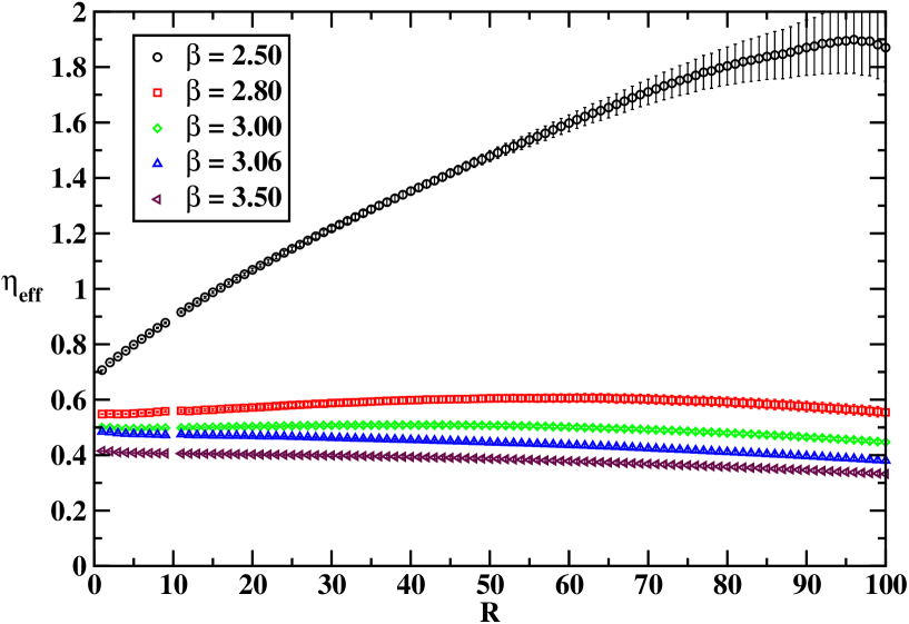
Figure 4: $\eta_{\mbox{\scriptsize eff}}$ vs $R$ on the lattice $200^{2}\times 8$ for several $\beta$ values.

The analysis of the behavior of $\eta_{\mbox{\scriptsize eff}}(R)$ has been repeated setting $\beta$ at our estimated value for $\beta_{c}$, i.e. $\beta=3.06$, and increasing the spatial extent of the lattice. It turns out (see Fig. 5) that a plateau develops at small distances when $L$ increases and that the extension of this plateau gets larger with $L$, consistently with the fact that finite volume effects are becoming less important. The plateau value of $\eta_{\mbox{\scriptsize eff}}$ can be estimated as $\eta_{\mbox{\scriptsize eff}}(R=6)$ on the 256${}^{2}\times 8$ lattice and is equal to 0.4782(25); it agrees with our previous determination of the index $\eta$.

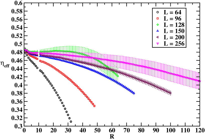
Figure 5: $\eta_{\mbox{\scriptsize eff}}$ vs $R$ at $\beta_{c}$ on lattices with several values of $L$.

The scenario described by Fig. 5 for $\beta=\beta_{c}$ must be valid for any $\beta>\beta_{c}$, if the system undergoes a BKT transition, since the correlator must obey a power law in the whole high-$\beta$ phase. We have found that this is indeed the case by performing an analysis similar to that shown in Fig. 5 at several $\beta$ values larger than $\beta_{c}$ (see Fig. 6 for the case of $\beta=3.50$, which leads to $\eta\approx 0.41$)). We observe that, in general, $\eta(\beta)<\eta(\beta_{c})$ for $\beta>\beta_{c}$ and had we estimated $\beta_{c}$ from the 3-parameter fit with $L_{\mbox{\scriptsize min}}=64$, instead of that with $L_{\mbox{\scriptsize min}}=96$, i.e. 3.44(15) instead of 3.06(11), the resulting $\eta$ would change by little and keep still much larger than the $XY$ value 0.25.

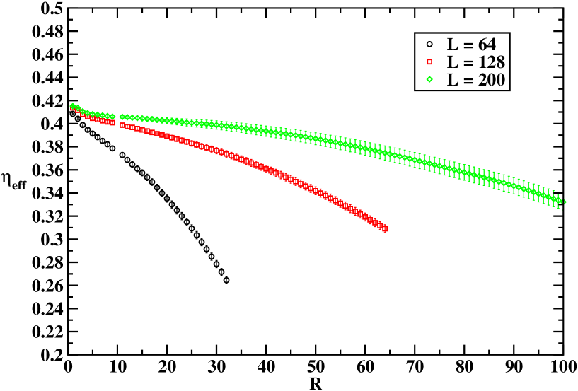
Figure 6: $\eta_{\mbox{\scriptsize eff}}$ vs $R$ at $\beta=3.50$ on lattices with several values of $L$.

4 Discussions

In this paper we have studied the critical behavior of the $3d$ $U(1)$ LGT at finite temperature. We worked on isotropic lattice with the temporal extension $N_{t}=8$. The pseudo-critical coupling was determined through the peak in the susceptibility of the Polyakov loop. The infinite-volume critical coupling has then been computed assuming the scaling behavior of the form (8). Our fitting gives the value $\beta_{c}=3.06(11)$. The deconfinement phase is the phase where $\beta\geq\beta_{c}$. The detailed study of the deconfined phase is clearly beyond the scope of the present paper. Nevertheless, this finding has immediate impact on the previous studies of the model. A thorough investigation of the deconfinement phase was performed in Ref. [8]. However, all $\beta$-values used there are smaller than the infinite-volume critical coupling. When the thermodynamic limit is approached the critical coupling increases so that the numerical results of Ref. [8] would refer rather to the confinement phase of the infinite-volume theory. This is indeed the case as we explained in the previous section. One sees from Fig. 3 that the correlation length (inverse of the string tension) grows till the pseudo-critical value of $\beta$ is reached. Therefore, the string tension is non-vanishing for all values of $\beta$ used in Ref. [8]. We conclude the much larger $\beta$-values are needed than those used in Ref. [8] to really probe the physics of the deconfinement phase in the large volume limit. This however might call for very large lattice sizes so the feasibility of such a study is not clear at present.

Furthermore, the index $\nu$ has been extracted from the scaling of the pseudo-critical couplings (8). Its value does agree well with the expected $XY$ value $\nu=1/2$. Of course, it would be desirable to extract this index directly from the correlation of the Polyakov loops along the line described in the previous section.

One of the main results of our paper is the computation of the index $\eta$ which turns out to be $\eta\approx 0.496$. This value is essentially larger than expected and requires some discussion. The easiest explanation would be to state that the spatial lattice size used ($L\in[32-256]$) is still too small to exhibit the correct scaling behavior, hence the wrong values for $\beta_{c}$ and $\eta$ follow. However, if one makes a plot of $\beta_{pc}(L)$ vs $L$, one can see, by looking at the trend of data, that it is unlikely that $\beta_{c}$ is much larger than our estimate. In fact, our fits with the scaling law (8) show that $\beta_{c}$ decreases when $L_{\mbox{\scriptsize min}}$ increases (see Table 2). Therefore, our result is most likely an overestimation. This implies that the true $\eta$ is likely even larger than what we found. In any case, even if we use for $\beta_{c}$ rather unlikely value $\beta_{c}=3.50$, Fig. 6 suggests that $\eta\approx 0.41$, much above the $XY$ value.

The next objection against our result could be the fact that we have neglected logarithmic corrections to the scaling law (9). It looks for us rather strange that logarithmic corrections can lead to decreasing $\eta$ almost by two times. We want to mention that including naively such corrections into our fits always results in the increasing of $\eta$ values, though these values are unstable against the maximal lattice size included into fit. Thus, although we cannot rule out this possibility, we do not think that neglecting logarithmic corrections results in such a wrong prediction for $\eta$.

Let us give a simple argument why the index $\eta$ can be different from its $XY$ value. Consider the anisotropic lattice. We would like to study the limit of large $\beta_{s}$. In the limit $\beta_{s}=\infty$ the spatial plaquettes are frozen to unity. That means, the ground state is a state where all spatial fields are pure gauge, i.e. $U_{n}(x)\ =\ V_{x}V^{*}_{x+e_{n}}\ ,\ n=1,2$. Perform now a change of variables $U_{0}(x)\to V_{x}U_{0}(x)V^{*}_{x+e_{0}}$. Then it is easy to see that in the leading order of the large-$\beta_{s}$ expansion the partition function factorizes into the product of $N_{t}$ independent $2d$ $XY$ models. Let us now look at the correlations of the Polyakov loops. Since the Polyakov loop is the product of gauge fields in the temporal direction, the correlation function factorizes, too, and becomes a product of independent $XY$ correlations, i.e.

$$\Gamma_{U(1)}(\beta_{s}=\infty,\beta_{t})\ =\ \left[\Gamma_{XY}(\beta_{t})\right]^{N_{t}}\ .$$ (12)

Hence, for asymptotically large $R\gg 1$, we get

$$\Gamma_{U(1)}(\beta_{s}=\infty,\beta_{t}\geq\beta_{t}^{cr})\ \asymp\ \left[\frac{1}{R^{\eta_{XY}}}\right]^{N_{t}}\ .$$ (13)

This leads to a simple relation

$$\eta(\beta_{s}=\infty,\beta_{t}^{cr})\ =\ N_{t}\ \eta_{XY}\ .$$ (14)

Some conclusions could now be drawn. The critical behavior of the $3d$ $U(1)$ LGT in the limit $\beta_{s}\to\infty$ is also governed by the $2d$ $XY$ model. Nevertheless, the effective index $\eta$ appears to be $N_{t}$ times of its $XY$ value. Now, for $\beta_{s}=0$ we have $\eta(\beta_{s}=0,\beta_{t}^{cr})\ =\ \eta_{XY}$. This relation and formula (14) allow to conjecture that

$$\eta_{XY}\ \leq\ \eta(\beta_{s},\beta_{t}^{cr})\ \leq\ N_{t}\ \eta_{XY}\ .$$ (15)

$\beta_{s}=0$ corresponds to the lower limit while $\beta_{s}=\infty$ corresponds to the upper limit. In general, $\eta$ could interpolate between two limits with $\beta_{s}$. Whether this interpolation is monotonic or there exists critical value $\beta_{s}^{cr}$, such that $\eta(\beta_{s}\leq\beta_{s}^{cr},\beta_{t}^{cr})\ =\ \eta_{XY}$ and $\eta$ changes monotonically above $\beta_{s}^{cr}$, cannot be answered with data we have and requires simulations on the anisotropic lattices. In the paper [11] a renormalization group study of $3d$ $U(1)$ model at small $\beta_{s}$ will be presented and computations of the leading correction to the large $\beta_{s}$ behavior will be given. The results of our computations support the scenario that the index $\eta$ depends on the ratio $\beta_{s}/\beta_{t}$. Recently, we have obtained the results of simulations for $N_{t}=2,4$ performed by A. Bazavov [12]. His results also point in the direction of our scenario (see Fig. 7). In Fig. 7 we plot a possible behavior of $\eta$ supposing the monotonic dependence.

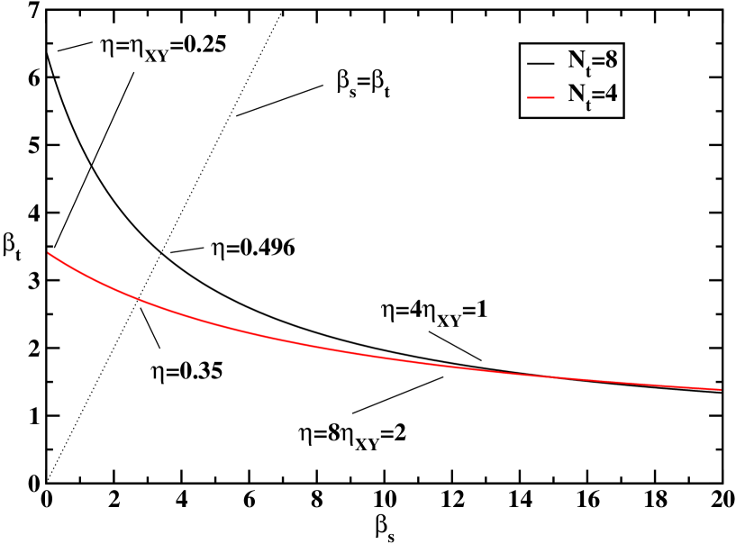
Figure 7: Conjectured behavior of $\eta$ in the $\beta_{s}$-$\beta_{t}$ plane. Results for $N_{t}=4$ are taken from Ref. [12].

Finally, it is worth mentioning that the factorization in the large $\beta_{s}$ limit does not affect the index $\nu$. It follows from its definition (4) that in this limit $\nu=1/2$ as in the $XY$ model. We expect therefore that $\nu$ equals $1/2$ for all $\beta_{s}$ and is thus universal.

In view of our results it might be worth to perform numerical simulations for small but nonvanishing $\beta_{s}$ and for larger volumes. The feasibility of a study with larger volumes and better accuracy relies strongly on the possibility to improve the simulation code. Promising directions could be simulations of the dual formulation of the model (possibly with a cluster algorithm) or the use of the Lüscher-Weisz algorithm [13]. The development of these directions is in progress.

Acknowledgment

O.B. thanks for warm hospitality the Dipartimento di Fisica dell’Università della Calabria and the INFN Gruppo Collegato di Cosenza during the work on this paper. Numerical simulations were performed on the linux PC farm “Majorana” of the INFN-Cosenza and on the GRID cluster at the ITP-Kiev. Authors would like to thank A. Bazavov for interesting discussions and for providing us with the results of his simulations on the lattices with $N_{t}=2,4$ prior to publication.

References

- [1] O. Borisenko, M. Gravina and A. Papa, J. Stat. Mech. 2008 (2008) P08009 [arXiv:0806.2081 [hep-lat]].
- [2] A. Polyakov, Nucl. Phys. B 120 (1977) 429; M. Göpfert, G. Mack, Commun. Math. Phys. 81 (1981) 97; 82 (1982) 545.
- [3] N. Parga, Phys. Lett. B 107 (1981) 442.
- [4] B. Svetitsky, L. Yaffe, Nucl. Phys B 210 (1982) 423.
- [5] V. L. Berezinskii, Sov. Phys. JETP 32 (1971) 493.
- [6] J. M. Kosterlitz and D. J. Thouless, J. Phys. C 6 (1973) 1181.
- [7] P. D. Coddington, A. J. G. Hey, A. A. Middleton and J. S. Townsend, Phys. Lett. B 175 (1986) 64.
- [8] M. N. Chernodub, E. M. Ilgenfritz, A. Schiller, Phys. Rev. D 64 (2001) 054507 [arXiv:hep-lat/0105021]; Phys. Rev. Lett. 88 (2002) 231601 [arXiv:hep-lat/0112048]; Phys. Rev. D 67 (2003) 034502 [arXiv:hep-lat/0208013].
- [9] R. Kenna and A. C. Irving, Nucl. Phys. B 485 (1997) 583.
- [10] M. Hasenbusch, J. Phys. A 38 (2005) 5869.
- [11] O. Borisenko, V. Chelnokov, Renormalization group study of lattice gauge theory in the finite temperature limit, in preparation.
- [12] A. Bazavov, private communication.
- [13] M. Luscher and P. Weisz, JHEP 0109 (2001) 010 [arXiv:hep-lat/0108014].