KUNS-2251 HRI/ST/1001

A Novel Large-$N$ Reduction on $S^{3}$:

Demonstration in Chern-Simons Theory

Goro Ishiki¹⁾, Shinji Shimasaki^2),3) and Asato Tsuchiya⁴⁾

¹⁾ Center for Quantum Spacetime (CQUeST)
Sogang University, Seoul 121-742, Korea
²⁾ Department of Physics, Kyoto University
Kyoto, 606-8502, Japan
³⁾ Harish-Chandra Research Institute
Chhatnag Road, Jhusi, Allahabad 211019, India
⁴⁾ Department of Physics, Shizuoka University
836 Ohya, Suruga-ku, Shizuoka 422-8529, Japan

We show that the planar Chern-Simons (CS) theory on $S^{3}$ can be described by its dimensionally reduced model. This description of CS theory can be regarded as a novel large-$N$ reduction for gauge theories on $S^{3}$. We find that if one expands the reduced model around a particular background consisting of multiple fuzzy spheres, the reduced model becomes equivalent to CS theory on $S^{3}$ in the planar limit. In fact, we show that the free energy and the vacuum expectation value of unknot Wilson loop in CS theory are reproduced by the reduced model in the large-$N$ limit.

1 Introduction

The large-$N$ reduction [1] asserts that large-$N$ gauge theories on flat space-times are equivalent to matrix models (reduced models) that are obtained by dimensional reduction to lower dimensions (for further developments, see [2, 3, 4, 5, 6]). It is not only conceptually relevant because it realizes emergent space-time in matrix models, but also practically relevant because it can give a non-perturbative formulation of planar gauge theories as an alternative to lattice gauge theories. It is well-known that the equivalence does not hold naively due to the $U(1)^{d}$ symmetry breaking [2]. Some remedy is needed for the equivalence to indeed hold (for recent studies, see [7, 8, 9, 10, 11]). However, as far as we know, there has been no remedy that manifestly preserves supersymmetry in gauge theories. Recently, the large-$N$ reduction was generalized to theories on $S^{3}$ in [12] (for earlier discussions, see [13, 14, 15]). Here $S^{3}$ is constructed as a nontrivial $U(1)$ fiber bundle over $S^{2}$ by expanding matrix models around a particular background corresponding to a sequence of fuzzy spheres. This novel large-$N$ reduction is important from both of the above two viewpoints. It would give hints to the problem of describing curved space-time [16] in the matrix models [17, 18, 19]. Unlike on flat space-times, the equivalence would hold on curved space-times without any remedy since the theories are massive due to the curvature of $S^{3}$. The novel large-$N$ reduction can, therefore, give a non-perturbative regularization of gauge theories that respects both supersymmetry and the gauge symmetry.

The novel large-$N$ reduction has been studied mainly for two cases so far. One is ${\cal N}=4$ SYM on $R\times S^{3}$ [12, 21, 22, 23]. The reduced model of this theory takes the form of the plane wave matrix model [24]. The large-$N$ reduction provides a non-perturbative formulation of ${\cal N}=4$ SYM, which respects sixteen supersymmetries and the gauge symmetry so that no fine tuning of the parameters is required. Thus the formulation gives a feasible way to analyze the strongly coupled regime of ${\cal N}=4$ SYM, for instance, by putting it on a computer through the methods proposed in [25, 26, 27], and therefore enables us to perform new nontrivial tests of the AdS/CFT correspondence [28, 29, 30].

The other is Chern-Simons (CS) theory on $S^{3}$, which has been exactly solved [31]. In this case, the equivalence between the reduced model and the original theory can be verified explicitly, which was briefly reported in [32]. In this paper, we present the verification of the equivalence in detail. We also discuss the large-$N$ reduction for CS theory on $S^{3}/Z_{q}$. Our result is an explicit demonstration of the novel large-$N$ reduction. CS theory on $S^{3}$ is a topological field theory associated with the knot theory and therefore interesting in its own right. Our formulation gives a new regularization method for CS theory on $S^{3}$. CS theory on $S^{3}$ is also interpreted as open topological A strings on $T^{\ast}S^{3}$ in the presence of $N$ D-branes wrapping $S^{3}$. Topological strings capture some aspects of more realistic string, so that our study is expected to give some insights into the matrix models as a non-perturbative formulation of superstring.

More recently, it was shown in [33] that the large-$N$ reduction holds on general group manifolds. In the case of $S^{3}\simeq SU(2)$, the background taken in the large-$N$ reduction in [33] is different from that in [12]. It is desirable to explicitly demonstrate this different type of the large-$N$ reduction, for instance, in the case of CS theory on $S^{3}$. We leave this for a future study.

This paper is organized as follows. In section 2, we briefly review CS theory on $S^{3}$. In section 3, we summarize the relationships among CS theory on $S^{3}$, 2d YM on $S^{2}$ and the matrix model which were obtained in [34, 35]. In section 4, we argue how CS theory on $S^{3}$ is realized in the matrix model as a novel large-$N$ reduction. In section 5, we show the equivalence between the theory around a particular background of the matrix model and CS theory on $S^{3}$. In section 6, by using the Monte Carlo simulation, we give a check of this equivalence. Section 7 is devoted to conclusion and discussion. In appendices, some details are gathered.

2 Chern-Simons theory on $S^{3}$

In this section, we review some known facts about CS theory on $S^{3}$ needed for this paper [36, 37]. We consider CS theory on $S^{3}$ with the gauge group $U(N)$, whose action is given by

$$S_{CS}=\frac{k}{4\pi}\int_{S^{3}}\mbox{Tr}\left(A\wedge dA+\frac{2}{3}A\wedge A\wedge A\right),$$ (2.1)

where $k$ must be an integer. The partition function

$${\cal Z}_{CS}=\int{\cal D}A\;e^{iS_{CS}}$$ (2.2)

defines a topological invariant of the manifold $S^{3}$, which also depends on a choice of framing. Given an oriented knot ${\cal K}$ in $S^{3}$, one can consider the Wilson loop in an irreducible representation $R$ of $U(N)$

$$W_{R}({\cal K})=\mbox{Tr}_{R}\left(P\exp\oint_{{\cal K}}A\right).$$ (2.3)

The expectation value of the Wilson loop

$$\langle W_{R}({\cal K})\rangle_{CS}=\frac{1}{{\cal Z}_{CS}}\int{\cal D}A\;W_{R}({\cal K})\;e^{iS_{CS}}$$ (2.4)

defines a topological invariant of ${\cal K}$ depending on a choice of framing as well. In this paper, we are concerned with the Wilson loop for the unknot, which we denote by $W_{R}(\mbox{unknot})$, and mainly consider the Wilson loop for the unknot in the fundamental representation, which we denote by $W_{\square}(\mbox{unknot})$.

$S^{3}$ is obtained by gluing two solid tori along their boundaries with the transformation

$$K=T^{m}ST^{n},$$ (2.5)

where $S$ and $T$ are generators of $SL(2,Z)$, and $m$ and $n$ are arbitrary integers. $T$ has the following representation in the Hilbert space ${\cal H}(T^{2})$, which is obtained by doing canonical quantization of CS theory on $R\times T^{2}$:

$$\langle R|T|R^{\prime}\rangle=\delta_{RR^{\prime}}T_{R},$$ (2.6)

$$T_{R}=\exp\left[\frac{2\pi i}{k+N}\left(\Lambda\cdot\rho+\frac{1}{2}\Lambda^{2}-\frac{1}{24}k(N^{2}-1)\right)\right],$$ (2.7)

where $|R\rangle$ denotes a state associated to the highest weight $\Lambda$, and $\rho$ is the Weyl vector of $SU(N)$. The partition function is given by

$${\cal Z}_{CS}=\langle 0|K|0\rangle,$$ (2.8)

where $0$ stands for the trivial representation, while the expectation value of the Wilson loop for the unknot is given by

$$\langle W_{R}(\mbox{unknot})\rangle_{CS}=\frac{\langle R|K|0\rangle}{\langle 0|K|0\rangle}.$$ (2.9)

The canonical framing corresponds to $m=n=0$. In the following, we first present the exact results for the partition function and the expectation value of the Wilson loop in the canonical framing. The partition function (2.2) was computed exactly:

$${\cal Z}_{CS}^{m=n=0} =\langle 0|S|0\rangle=\frac{1}{(k+N)^{N/2}}\sum_{w\in W}\varepsilon(w)\exp\left(-\frac{2\pi i}{k+N}\rho\cdot w(\rho)\right),$$ (2.10)

where the sum over $w$ is a sum over the elements of the Weyl group ${\cal W}$ of $U(N)$, and $\varepsilon(w)$ is the signature of $w$. The expectation value of the Wilson loop for the unknot was also computed exactly:

$$\langle W_{R}(\mbox{unknot})\rangle_{CS}^{m=n=0}=\frac{\langle R|S|0\rangle}{\langle 0|S|0\rangle}=\frac{\sum_{w\in W}\varepsilon(w)e^{-\frac{2\pi i}{k+N}\rho\cdot w(\Lambda+\rho)}}{\sum_{w\in W}\varepsilon(w)e^{-\frac{2\pi i}{k+N}\rho\cdot w(\rho)}}.$$ (2.11)

One can obtain different expressions for (2.10) and (2.11) by using Weyl’s character formula

$$\mbox{ch}_{R}(u)=\sum_{\mu\in M_{R}}e^{\mu\cdot u}=\frac{\sum_{w\in W}\varepsilon(w)e^{w(\Lambda+\rho)\cdot u}}{\prod_{\alpha>0}2\sinh\frac{\alpha\cdot u}{2}},$$ (2.12)

and Weyl’s denominator formula

$$\sum_{w\in W}\varepsilon(w)e^{w(\rho)\cdot u}=\prod_{\alpha>0}2\sinh\frac{\alpha\cdot u}{2},$$ (2.13)

where $\alpha>0$ are positive roots, and $M_{R}$ is the set of weights associated to the representation $R$. By applying (2.13) to (2.10), one obtains

$${\cal Z}_{CS}^{m=n=0}=\frac{1}{(k+N)^{N/2}}\prod_{\alpha>0}2\sinh\left(\frac{2\pi i}{k+N}\frac{\alpha\cdot\rho}{2}\right),$$ (2.14)

while by applying (2.12) and (2.13) to (2.11)

$$\langle W_{R}(\mbox{unknot})\rangle_{CS}^{m=n=0}=\mbox{ch}_{R}\left(-\frac{2\pi i}{k+N}\rho\right)=\prod_{\alpha>0}\frac{\sinh\left(\frac{2\pi i}{k+N}\frac{\alpha\cdot(\Lambda+\rho)}{2}\right)}{\sinh\left(\frac{2\pi i}{k+N}\frac{\alpha\cdot\rho}{2}\right)}.$$ (2.15)

For the fundamental representation, it reduces to

$$\langle W_{\square}(\mbox{unknot})\rangle_{CS}^{m=n=0}=\frac{\sinh\frac{\pi iN}{k+N}}{\sinh\frac{\pi i}{k+N}}.$$ (2.16)

Furthermore, by using (2.13), one can show that (2.10) is equivalent to an integral over $N$ variables which takes the form analogous to a partition function of a matrix model [38, 39, 36]:

$${\cal Z}_{CS}^{m=n=0}={\cal Z}_{CSM}=\frac{e^{-\frac{g_{s}}{12}N(N^{2}-1)}}{N!}\int\prod_{i=1}^{N}\frac{d\beta_{i}}{2\pi}e^{-\frac{1}{2g_{s}}\sum_{i}\beta_{i}^{2}}\prod_{i<j}\left(2\sinh\frac{\beta_{i}-\beta_{j}}{2}\right)^{2},$$ (2.17)

where we have introduced

$$g_{s}=\frac{2\pi i}{k+N},$$ (2.18)

which is identified with the string coupling in the context of topological strings. We call the statistical model defined by (2.17) the Chern-Simons matrix model (CS matrix model). Correspondingly, one can find a relation

$$\langle W_{R}(\mbox{unknot})\rangle_{CS}^{m=n=0}=e^{-g_{s}(\rho\cdot\Lambda+\frac{1}{2}\Lambda^{2})}\langle\mbox{ch}_{R}(\beta)\rangle_{CSM}=e^{-g_{s}(\rho\cdot\Lambda+\frac{1}{2}\Lambda^{2})}\left\langle\sum_{\mu\in M_{R}}e^{\mu\cdot\beta}\right\rangle_{CSM}$$ (2.19)

where

$$\langle\cdots\rangle_{CSM}=\frac{1}{Z_{CSM}}\frac{e^{-\frac{1}{12}N(N^{2}-1)}}{N!}\int\prod_{i=1}^{N}\frac{d\beta_{i}}{2\pi}(\cdots)\>e^{-\frac{1}{2g_{s}}\sum_{i}\beta_{i}^{2}}\prod_{i<j}\left(2\sinh\frac{\beta_{i}-\beta_{j}}{2}\right)^{2}.$$ (2.20)

Finally we consider the framing with $m=n=1$, which appears in the direct evaluation of the partition function of CS theory on $S^{3}$ in [40]. One can see from (2.8) that the partition function in this framing is related to the one in the canonical framing as

$${\cal Z}_{CS}^{m=n=1} =T_{0}^{2}{\cal Z}_{CS}^{m=n=0}$$

$$=\frac{e^{-\frac{\pi i}{6}(N^{2}-1)+\frac{g_{s}}{12}N(N^{2}-1)}}{(k+N)^{N/2}}\prod_{\alpha>0}2\sinh\left(\frac{2\pi i}{k+N}\frac{\alpha\cdot\rho}{2}\right)$$

$$=\frac{e^{-\frac{\pi i}{6}(N^{2}-1)}}{N!}\int\prod_{i=1}^{N}\frac{d\beta_{i}}{2\pi}e^{-\frac{1}{2g_{s}}\sum_{i}\beta_{i}^{2}}\prod_{i<j}\left(2\sinh\frac{\beta_{i}-\beta_{j}}{2}\right)^{2}.$$ (2.21)

One can also see from (2.9) that the expectation value of the Wilson loop is related to the one in the canonical framing as

$$\langle W_{R}(\mbox{unknot})\rangle_{CS}^{m=n=1}=\frac{T_{R}}{T_{0}}\langle W_{R}(\mbox{unknot})\rangle_{CS}^{m=n=0}=\langle\mbox{ch}_{R}(\beta)\rangle_{CSM}=\left\langle\sum_{\mu\in M_{R}}e^{\mu\cdot\beta}\right\rangle_{CSM}.$$ (2.22)

In particular, because $\Lambda\cdot\rho+\frac{1}{2}\Lambda^{2}=\frac{N^{2}-1}{2N}$ for the fundamental representation, one obtains

$$\langle W_{\square}(\mbox{unknot})\rangle_{CS}^{m=n=1}=e^{\frac{g_{s}}{2}\left(N-\frac{1}{N}\right)}\frac{\sinh\frac{g_{s}N}{2}}{\sinh\frac{g_{s}}{2}}.$$ (2.23)

Similarly, the perturbative part of the free energy is evaluated in this framing as

$${\cal F}_{CS}=\frac{g_{s}}{12}N(N^{2}-1)+\sum_{j=1}^{N}(N-j)\sum_{n=1}^{\infty}\log\left(1+\frac{j^{2}g_{s}^{2}}{4\pi^{2}n^{2}}\right).$$ (2.24)

In the following sections, we will show that the reduced model of CS theory on $S^{3}$ reproduces the results for the original theory in the framing corresponding $m=n=1$.

3 CS theory on $S^{3}$, 2d YM on $S^{2}$ and a matrix model

In this section, we review part of the results in [34, 35], which we use in this paper. In section 3.1, we dimensionally reduce CS theory on $S^{3}$ to 2d YM on $S^{2}$ and a matrix model. In section 3.2, we describe a classical equivalence between the theory around each multiple monopole background of 2d YM on $S^{2}$ and the theory around a certain multiple fuzzy sphere background of the matrix model. In section 3.3, we exactly perform the integration in the matrix model. In section 3.4, using the result in section 3.3, we show that the equivalence in section 3.2 also holds at quantum level.

3.1 Dimensional reductions

In order to dimensionally reduce CS theory on $S^{3}$, we expand the gauge field in terms of the right-invariant 1-form defined in (A.3) as

$$A=iX_{i}E^{i}.$$ (3.1)

We choose an $SO(4)$-isometric metric for $S^{3}$ (A.6) fixing the radius of $S^{3}$ to $2/\mu$. Then, we rewrite (2.1) as

$$S_{CS}=-\frac{k}{4\pi}\int\frac{d\Omega_{3}}{(\mu/2)^{3}}\mbox{Tr}\left(i\mu\epsilon^{ijk}X_{i}{\cal L}_{j}X_{k}+\mu X_{i}^{2}+\frac{2i}{3}\epsilon^{ijk}X_{i}X_{j}X_{k}\right),$$ (3.2)

where ${\cal L}_{i}$ is the Killing vector dual to $E^{i}$ defined in (A.7), and we have used the Maurer-Cartan equation (A.5).

As we explain in appendix A, we regard $S^{3}$ as a $U(1)$ bundle over $S^{2}$. Here the fiber direction is parametrized by $y$. By dropping the $y-$derivatives, we obtain a gauge theory on $S^{2}$:

$$S_{BF}=\frac{\mu}{2g_{YM}^{2}}\int\frac{d\Omega_{2}}{\mu^{2}}\mbox{Tr}\left(i\mu\epsilon^{ijk}X_{i}L_{j}X_{k}+\mu X_{i}^{2}+\frac{2i}{3}\epsilon^{ijk}X_{i}X_{j}X_{k}\right),$$ (3.3)

where $g_{YM}^{2}=-\frac{\mu^{2}}{2k}$, the radius of $S^{2}$ is $1/\mu$, and $L_{i}$ are the angular momentum operators on $S^{2}$ given in (A.13) with $q=0$. $g_{YM}$ will be identified with the coupling constant of 2d YM on $S^{2}$ below. First, we see that (3.3) is the BF theory with a mass term on $S^{2}$. We expand $X_{i}$ as [41, 15]

$$\vec{X}=\mu\left(\chi\vec{e}_{r}+a_{\theta}\vec{e}_{\varphi}-\frac{1}{\sin\theta}a_{\varphi}\vec{e}_{\theta}\right),$$ (3.4)

where $\vec{e}_{r}=(\sin\theta\cos\varphi,\sin\theta\sin\varphi,\cos\theta)$ and $\vec{e}_{\theta}=\frac{\partial\vec{e}_{r}}{\partial\theta}$, $\vec{e}_{\varphi}=\frac{1}{\sin\theta}\frac{\partial\vec{e}_{r}}{\partial\varphi}$. $a_{\mu}$ are the gauge field on $S^{2}$, and $\chi$ is a scalar field on $S^{2}$ which comes from the component of the fiber direction of the gauge field on $S^{3}$. Indeed, we can rewrite (3.3) as

$$S_{BF}=\frac{\mu^{4}}{2g_{YM}^{2}}\int\frac{d\Omega_{2}}{\mu^{2}}\mbox{Tr}\left(\chi\epsilon^{\mu\nu}f_{\mu\nu}-\chi^{2}\right),$$ (3.5)

where $f_{\mu\nu}=\partial_{\mu}a_{\nu}-\partial_{\nu}a_{\mu}+i[a_{\mu},a_{\nu}]$ is the field strength. This is the BF theory with a mass term: the first term is the BF term and the second term is a mass term. Next, we integrate $\chi$ out in (3.5) to obtain 2d YM on $S^{2}$:

$$S_{YM}=\frac{\mu^{4}}{g_{YM}^{2}}\int\frac{d\Omega_{2}}{\mu^{2}}\mbox{Tr}\left(\frac{1}{4}f^{\mu\nu}f_{\mu\nu}\right).$$ (3.6)

Furthermore, by dropping all the derivatives in (3.3) and rescale $X_{i}$ as $X_{i}\rightarrow\mu X_{i}$, we obtain a three-matrix model:

$$S_{m}=-\frac{1}{g_{m}^{2}}\mbox{Tr}\left(X_{i}^{2}+\frac{i}{3}\epsilon^{ijk}X_{i}[X_{j},X_{k}]\right),$$ (3.7)

where $1/g_{m}^{2}=-2\pi\mu^{2}/g_{YM}^{2}$. In the sense of the Dijkgraaf-Vafa theory [42], this matrix model is regarded as a mass deformed superpotential of ${\cal N}=4$ SYM, which gives the so-called ${\cal N}=1^{*}$ theory.

3.2 Classical equivalence between 2d YM on $S^{2}$ and the matrix model

The matrix model (3.7) with the matrix size $M\times M$ possesses the following classical solution,

$$\hat{X}_{i}=L_{i}=\bigoplus_{s}L^{[j_{s}]}_{i}\otimes 1_{N_{s}}$$ (3.8)

where $L^{[j_{s}]}_{i}$ are the spin $j_{s}$ representation of the $SU(2)$ generators obeying $[L^{[j_{s}]}_{i},L^{[j_{s}]}_{j}]=i\epsilon_{ijk}L^{[j_{s}]}_{k}$, and the relation $\sum_{s}(2j_{s}+1)N_{s}=M$ is satisfied. $s$ runs over some integers, but its range is not specified here. It will be specified later as $-\Lambda/2\leq s\leq\Lambda/2$ with $\Lambda$ an even positive integer.

We put $2j_{s}+1=\Omega+n_{s}$ with $\Omega$ and $n_{s}$ integers and take the limit in which

$$\Omega\rightarrow\infty\;\;\;\mbox{with}\;\;\;\frac{\Omega}{g_{m}^{2}}=-\frac{8\pi^{2}}{g_{YM}^{2}A}=\mbox{fixed},$$ (3.9)

where $A=4\pi/\mu^{2}$ is the area of $S^{2}$. Then, it was shown classically in [34] that the theory around (3.8) is equivalent to the theory around the following classical solution of (3.3) with the gauge group $U(K)$,

$$\mu L_{i}+\hat{X}_{i}=\mu\mbox{diag}(\cdots,\underbrace{L^{(q_{s})}_{i},\cdots,L^{(q_{s})}_{i}}_{N_{s}},\cdots),$$ (3.10)

where $q_{s}=n_{s}/2$, and $\sum_{s}N_{s}=K$ is satisfied. $L^{(q_{s})}_{i}$ are the angular momentum operators in the presence of a monopole with the monopole charge $q_{s}$, which are given in (A.13). This theory can also be viewed as the theory around the following classical solution of (3.5),

$$\hat{\chi}=-\mbox{diag}(\cdots,\underbrace{q_{s},\cdots,q_{s}}_{N_{s}},\cdots),$$

$$\hat{a}_{\theta}=0,$$

$$\hat{a}_{\varphi}=(\cos\theta\mp 1)\hat{\chi},$$ (3.11)

where the upper sign is taken in the region $0\leq\theta<\pi$ and the lower sign in the region $0<\theta\leq\pi$, and $\hat{a}_{\theta}$ and $\hat{a}_{\varphi}$ represent the monopole configuration. Equivalently, this theory can be viewed as the theory around the multiple monopole background with the background for the gauge field given in (3.11) of 2d YM on $S^{2}$ (3.6). As reviewed in the following two subsections, the above equivalence is extended to quantum level [35].

3.3 Exact integration of the matrix model

First, we rewrite the matrix model (3.7) in terms of the following matrices;

$$Z =X_{1}+iX_{2},$$

$$\Phi =X_{3},$$ (3.12)

where $Z$ is an $M\times M$ complex matrix and $\Phi$ is an $M\times M$ hermitian matrix. The partition function is defined by

$${\cal Z}_{m} =\frac{1}{{\rm vol}(U(M))}\int dZdZ^{\dagger}d\Phi e^{iS_{m}},$$ (3.13)

$$S_{m} =-\frac{1}{g_{m}^{2}}\mbox{tr}\left\{Z[\Phi,Z^{\dagger}]+(1-i\epsilon)ZZ^{\dagger}+(1-i\epsilon)\Phi^{2}\right\}.$$ (3.14)

Here, in order to make the path integral well-defined and converge, we introduce $i$ in the exponential and $-i\epsilon$ in the action. Taking the gauge in which $\Phi$ is diagonal as $\Phi=\mathop{\rm diag}\nolimits(\phi_{1},\phi_{2},\cdots,\phi_{M})$ and integrating $Z$ and $Z^{\dagger}$ out, then we obtain

$${\cal Z}_{m}=\frac{1}{(2\pi)^{M}M!}\left(\frac{g_{m}^{2}\pi}{i}\right)^{M^{2}}\int\prod_{i}d\phi_{i}\prod_{i\neq j}\frac{\phi_{i}-\phi_{j}}{\phi_{i}-\phi_{j}+1-i\epsilon}e^{-\frac{i}{g_{m}^{2}}(1-i\epsilon)\sum_{i}\phi_{i}^{2}},$$ (3.15)

where $\prod_{i\neq j}(\phi_{i}-\phi_{j})$ comes from the diagonalization of $\Phi$, which is the square of the Vandermonde determinant. $(2\pi)^{M}$ is the volume of $U(1)^{M}$ and $M!$ is the volume of the Weyl group of $U(M)$.

Next let us concentrate on the factor in the integrand in (3.15),

$$\prod_{i\neq j}\frac{\phi_{i}-\phi_{j}}{\phi_{i}-\phi_{j}+1-i\epsilon}.$$ (3.16)

For this factor, we use the following formula,

$$\frac{1}{x-i\epsilon}=P.V.\frac{1}{x}+i\pi\delta(x),$$ (3.17)

where “$P.V.$” denotes the principal value. Then we obtain

$$\prod_{i\neq j}\frac{\phi_{i}-\phi_{j}}{\phi_{i}-\phi_{j}+1-i\epsilon}$$

$$=\prod_{i<j}\left[P.V.\frac{(\phi_{i}-\phi_{j})(\phi_{j}-\phi_{i})}{(\phi_{i}-\phi_{j}+1)(\phi_{j}-\phi_{i}+1)}+\left(-\frac{i\pi}{2}\right)\delta(\phi_{i}-\phi_{j}+1)+\left(-\frac{i\pi}{2}\right)\delta(\phi_{j}-\phi_{i}+1)\right].$$ (3.18)

It is easily seen that (3.18) is written in the sum of terms containing

$$\left(-\frac{i\pi}{2}\right)^{2j_{1}}\delta(\phi_{1}^{(1)}-\phi_{2}^{(1)}-1)\delta(\phi_{2}^{(1)}-\phi_{3}^{(1)}-1)\cdots\delta(\phi_{2j_{1}}^{(1)}-\phi_{2j_{1}+1}^{(1)}-1)$$

$$\times\left(-\frac{i\pi}{2}\right)^{2j_{2}}\delta(\phi_{1}^{(2)}-\phi_{2}^{(2)}-1)\delta(\phi_{2}^{(2)}-\phi_{3}^{(2)}-1)\cdots\delta(\phi_{2j_{2}}^{(2)}-\phi_{2j_{2}+1}^{(2)}-1)$$

$$\times\cdots$$

$$\times\left(-\frac{i\pi}{2}\right)^{2j_{K}}\delta(\phi_{1}^{(K)}-\phi_{2}^{(K)}-1)\delta(\phi_{2}^{(K)}-\phi_{3}^{(K)}-1)\cdots\delta(\phi_{2j_{K}}^{(K)}-\phi_{2j_{K}+1}^{(K)}-1),$$ (3.19)

where $K$ can take the value $1,2,\cdots,M$ and we have reordered and relabeled the eigenvalues of $\Phi$ as

$$\Phi=\mathop{\rm diag}\nolimits(\phi_{1}^{(1)},\cdots,\phi_{2j_{1}+1}^{(1)},\phi_{1}^{(2)},\cdots,\phi_{2j_{2}+1}^{(2)},\cdots,\phi_{1}^{(K)},\cdots,\phi_{2j_{K}+1}^{(K)}).$$ (3.20)

The size of the matrices, $M$, satisfies $M=\sum_{I=1}^{K}(2j_{I}+1)$. $\phi_{i}^{(I)}$ represents the $i$-th component of the $I$-th block. Thus (3.18) is decomposed into terms, each of which is characterized by an $M$-dimensional reducible representation of the $SU(2)$ algebra consisting of $K$ blocks (irreducible representations), with a $U(1)$ degree of freedom in each block. We label the reducible representations by “$r$” and denote the $U(1)$ part in the $I$-th block by $a_{I}$, putting $a_{I}\equiv\phi_{2j_{I}+1}^{(I)}+j_{I}$. Then, we obtain

$${\cal Z}_{m} =\sum_{r}\frac{{\cal N}_{r}}{(2\pi)^{M}}(-i\pi)^{M-N}\left(\frac{g_{m}^{2}\pi}{i}\right)^{M^{2}}\prod_{I=1}^{K}\frac{1}{2j_{I}+1}P.V.\int\prod_{I=1}^{K}da_{I}$$

$$\qquad\qquad\times\prod_{I\neq J}\prod_{m_{I}=-j_{I}}^{j_{I}}\prod_{m_{J}=-j_{J}}^{j_{J}}\frac{a_{I}+m_{I}-a_{J}-m_{J}}{a_{I}+m_{I}-a_{J}-m_{J}+1}e^{-\frac{i}{g_{m}^{2}}(1-i\epsilon)\sum_{I=1}^{K}\sum_{m_{I}=-j_{I}}^{j_{I}}(a_{I}+m_{I})^{2}},$$ (3.21)

where

$${\cal N}_{r}\equiv\prod\frac{1}{(\text{$\sharp$ of blocks with the same length})!}.$$ (3.22)

After some calculations, we find that (3.21) results in

$${\cal Z}_{m} =\sum_{r}\frac{{\cal N}_{r}}{(2\pi)^{M}}(-i\pi)^{M-N}\left(\frac{g_{m}^{2}\pi}{i}\right)^{M^{2}}\prod_{s=1}^{N}\frac{1}{2j_{s}+1}e^{-\frac{i}{3g_{m}^{2}}(1-i\epsilon)\sum_{I=1}^{K}j_{I}(j_{I}+1)(2j_{I}+1)}$$

$$\qquad\times P.V.\int\prod_{I=1}^{K}da_{I}\prod_{I<J}\frac{(a_{I}-a_{J})^{2}-(j_{I}-j_{J})^{2}}{(a_{I}-a_{J})^{2}-(j_{I}+j_{J}+1)^{2}}e^{-\frac{i}{g_{m}^{2}}(1-i\epsilon)\sum_{I=1}^{K}(2j_{I}+1)a_{I}^{2}}$$ (3.23)

Thus the partition function of the matrix model is decomposed into sectors characterized by the (reducible) representation of the $SU(2)$ algebra. Note that $P.V.$ prevents the integration over the $U(1)$ part $a_{I}$ from mixing the sectors.

3.4 2d YM on $S^{2}$ from the matrix model

In this subsection, we show that the partition function of YM on $S^{2}$ is obtained from that of the matrix model [35]. As we will see, the sector which consists of $K$ irreducible representations in the matrix model corresponds to $SU(K)$ 2d YM on $S^{2}$. In the $K$ block sector, we group the irreducible representations with the same dimension and label the groups by $s$, such that $j_{s}\neq j_{t}$ for $s\neq t$. We denote the multiplicity of the $s$-th group by $N_{s}$. Then, the relations $K=\sum_{s}N_{s}$ and $M=\sum_{s}N_{s}(2j_{s}+1)$ are satisfied. We also denote the $i$-th $U(1)$ part in the $s$-th group by $a_{si}$, where $i=1,\cdots,N_{s}$. Note that in this notation ${\cal N}_{r}$ in (3.22) equals $1/(\prod_{s}N_{s}!)$.

Since the partition function of the matrix model (3.23) is completely decomposed into sectors without overlap, we can extract the sectors consisting of $K$ blocks. In the $K$-block sector, due to the factor $\exp(-\frac{i}{3g_{m}^{2}}(1-i\epsilon)\sum_{I=1}^{K}j_{I}(j_{I}+1)(2j_{I}+1))$, configurations of almost equal size blocks are dominant in the limit in which $M/K=\Omega\rightarrow\infty,\;g_{m}^{2}/\Omega=\text{fixed}$. So, we consider configurations around the dominated configuration by setting

$$2j_{s}+1=\Omega+n_{s},$$ (3.24)

where $|n_{s}|\ll\Omega$. Substituting this into the $K$-block sector in (3.23) and taking the limit (3.9), we obtain

$${\cal Z}_{K\text{-block}} =C\sum_{\{n_{s},N_{s}\}}\int\prod_{s}\prod_{i=1}^{N_{s}}da_{si}\prod_{s\leq t}\prod_{i=1}^{N_{s}}\prod_{j=1}^{N_{t}}\left\{(a_{si}-a_{tj})^{2}-\frac{1}{4}(n_{s}-n_{t})^{2}\right\}$$

$$\hskip 199.16928pt\times e^{-i\frac{8\pi^{2}}{g_{YM}^{2}A}\sum_{s}\sum_{i=1}^{N_{s}}\left({a_{si}}^{2}+\frac{n_{s}^{2}}{4}\right)}.$$ (3.25)

Here we have absorbed overall irrelevant constants and divergences into a renormalized constant $C$. We have also replaced the denominator in the integrand in (3.23) by constant ($\Omega^{2}$) and taken the integral regions of $a_{si}$ to $(-\infty,\infty)$, since the exponential factor in (3.23) oscillates rapidly around $|a_{si}|\gtrsim\Omega$ in the limit where $\epsilon\rightarrow 0$ and $\Omega\rightarrow\infty$, so that the integral dominates around $|a_{si}|\ll\Omega$.

Finally, by rescaling $a_{si}$ by $y_{si}\equiv 2a_{si}$, and making an analytical continuation $g_{YM}^{2}\rightarrow-ig_{YM}^{2}$, we obtain

$${\cal Z}_{K} =C^{\prime}\sum_{\{n_{s},N_{s}\}}\int\prod_{s}\prod_{i=1}^{N_{s}}dy_{si}\prod_{s\leq t}\prod_{i=1}^{N_{s}}\prod_{j=1}^{N_{t}}\left\{(y_{si}-y_{tj})^{2}-(n_{s}-n_{t})^{2}\right\}$$

$$\hskip 284.52756pt\times e^{-\frac{2\pi^{2}}{g_{YM}^{2}A}\sum_{s}\sum_{i=1}^{N_{s}}(y_{si}^{2}+n_{s}^{2})},$$ (3.26)

where irrelevant constants are again absorbed into a constant $C^{\prime}$. ${\cal Z}_{K}$ exactly agrees with the partition function of $U(K)$ 2d YM on $S^{2}$ [43, 44, 45, 46, 47]. In YM on $S^{2}$, $n_{s}$ are identified with the monopole charges since the $n_{s}$ dependent term in the exponential coincides with the contribution of the classical solution (3.11) to the action of 2d YM. This fact is consistent with the classical equivalence reviewed in section 3.2.

4 CS theory on $S^{3}$ from the matrix model

In this section, we provide a prescription for realization of CS theory on $S^{3}$ in 2d YM on $S^{2}$ and in the matrix model. We also generalize the prescription to CS theory on $S^{3}/Z_{q}$. In section 5, we prove the large-$N$ equivalence between CS theory and the matrix model based on this prescription.

CS theory on $S^{3}$ is realized from 2d YM on $S^{2}$ through the large-$N$ reduction for the case of compact space proposed in [12] as follows. Note that the Kaluza-Klein (KK) momenta along the fiber ($S^{1}$) direction in $S^{3}$ are regarded as the monopole charges on $S^{2}$. Hence, if one considers the particular monopole solution in 2d YM on $S^{2}$ such that the spectrum of the monopole charges reproduces the spectrum of the KK momenta along $S^{1}$, the theory on $S^{2}$ expanded around such monopole solution is equivalent to CS theory on $S^{3}$. More precisely, in order to realize CS theory on $S^{3}$, we first put $n_{s}=s$ and $N_{s}=N$ in (3.10) (or in (3.11)) and then make $s$ run from $-\Lambda/2$ to $\Lambda/2$, where $\Lambda$ is a positive even integer. Finally we take the following limit,

$$\Lambda\rightarrow\infty,\;\;\;N\rightarrow\infty,\;\;\;-\frac{g_{YM}^{2}AN}{2\pi}=\frac{N}{k+N}=\mbox{fixed}.$$ (4.1)

Then, we see that 2d YM on $S^{2}$ expanded around the monopole background is equivalent to $U(N)$ CS theory on $S^{3}$ in the planar limit. Here, we can identify the difference of the monopole charges $n_{s}-n_{t}=s-t$ with the momenta $n\in Z$ along the $S^{1}$ fiber direction and $\Lambda$ is interpreted as the momentum cutoff. Introducing $N$ and taking the limit $N\rightarrow\infty$ are needed to suppress the non-planar contribution [12]. As for the relation between the coupling constants of the two theories, we naively expect that $-\frac{g_{YM}^{2}AN}{2\pi}=\frac{N}{k}=\mbox{fixed}$. However, the last relation in (4.1) implies that we need some renormalization. In sections 5 and 6, we show that the above prescription including the renormalization of the coupling constant is indeed valid.

Furthermore, by combining this equivalence with the relationship between 2d YM on $S^{2}$ and the matrix model reviewed in section 3.4, we obtain the following statement: if one takes in (3.8)

$$-\frac{\Lambda}{2}\leq s\leq\frac{\Lambda}{2},$$

$$2j_{s}+1=\Omega+s,$$

$$N_{s}=N$$ (4.2)

and takes the limit in which

$$\Omega\rightarrow\infty,\;\;\;\Lambda\rightarrow\infty,\;\;\;\Omega-\frac{\Lambda}{2}\rightarrow\infty,\;\;\;N\rightarrow\infty,$$

$$\frac{g_{m}^{2}N}{\Omega}=\frac{N}{4\pi(k+N)}=\mbox{fixed},$$ (4.3)

the theory around (3.8) of the matrix model (3.7) is equivalent to $U(N)$ CS theory on $S^{3}$ in the planar limit. In sections 5 and 6, we confirm this statement. The particular background (4.2) and the limit (4.3) is the same as the ones adopted in realizing ${\cal N}=4$ SYM on $R\times S^{3}$ in PWMM [12]. $\Omega$ and $\Lambda$ play the role of the ultraviolet cutoffs for the angular momenta on $S^{2}$ and in the fiber direction, respectively.

The results in section 3.4 and the above prescriptions lead us to consider the following statistical model,

$${\cal Z}=\int\prod_{s=-\Lambda/2}^{\Lambda/2}\prod_{i=1}^{N}dy_{si}\prod_{-\Lambda/2\leq s\leq t\leq\Lambda/2}\prod_{i,j=1}^{N}\{(y_{si}-y_{tj})^{2}+(s-t)^{2}\}e^{-\frac{1}{g^{2}}\sum_{s=-\Lambda/2}^{\Lambda/2}\sum_{i=1}^{N}y_{si}^{2}}.$$ (4.4)

This model is obtained from (3.26) by making an analytic continuation as $y_{si}\rightarrow iy_{si}$, $g^{2}\rightarrow-g^{2}$ and putting $n_{s}=s$, $N_{s}=N$ ($s=-\Lambda/2,\cdots,\Lambda/2$) . It follows from the above arguments that this model reproduces the planar limit of CS theory on $S^{3}$ in the limit in which

$$\Lambda\rightarrow\infty,\;\;\;N\rightarrow\infty$$ (4.5)

with

$$2\pi^{2}g^{2}N=\frac{2\pi iN}{k+N}=g_{s}N=\mbox{fixed}.$$ (4.6)

In the next section, we will verify the equivalence of CS theory on $S^{3}$ with (4.4) which is equivalent to the reduced matrix model expanded around the particular background.

We can easily extend the above argument to CS theory on $S^{3}/Z_{q}$. We consider the case in which $Z_{q}$ acts on the circle along the fiber direction in $S^{3}$. If we use the notation in appendix A, the periodicity for $S^{3}/Z_{q}$ is expressed as,

$$(\theta,\varphi,\psi)\sim(\theta,\varphi+2\pi,\psi+2\pi)\sim(\theta,\varphi,\psi+4\pi/q),$$ (4.7)

so that the radius of the fiber direction is $1/q$ of that for $q=1$ and the momenta along the fiber direction are discretized as $0,\pm q,\pm 2q,\cdots$. Then, we see that if one imposes (4.2) with the second equation replaced with $2j_{s}+1=\Omega+qs$ and takes the limit (4.3), the theory around (3.8) of the matrix model (3.7) is equivalent to $U(N)$ CS theory on $S^{3}/Z_{q}$ in the planar limit. Correspondingly, the statistical model for CS theory on $S^{3}/Z_{q}$ is given by replacing $s,t$ in (4.4) with $qs,qt$.

5 Proof of equivalence

In this section, we prove our statement that the model (4.4) reproduces the planar limit of CS theory on $S^{3}$ in the limit shown in (4.5) and (4.6). This equivalence can be understood from a correspondence between the Feynman diagrams in the two theories. The Feynman diagrams in (4.4) have a one-to-one correspondence to those in (2.17) which was obtained by rewriting the partition function of CS theory on $S^{3}$. Furthermore, if one takes the limit given by (4.5) and (4.6), each Feynman diagram in (4.4) takes the same value as the corresponding diagram in (2.17). We consider the free energy and the vacuum expectation value of unknot Wilson loop operator in the model (4.4) to see the equivalence. We show that they coincide with the results in CS theory on $S^{3}$ completely in the planar limit.

5.1 Feynman rule for our matrix model

Let us first consider the Feynman rule of (4.4). For this purpose, we rewrite (4.4) into a manifestly $U(N)$ invariant form. We will see that the result is given by a multi-matrix model with double trace interaction. This form allows us to compare the two theories explicitly.

We first factorize the measure in (4.4) as follows,

$$\prod_{s\leq t}\prod_{i,j}\{(y_{si}-y_{tj})^{2}+(s-t)^{2}\}=\sum_{s<t}(s-t)^{2N^{2}}\prod_{s}\prod_{i<j}(y_{si}-y_{sj})^{2}\prod_{s<t}\prod_{i,j}\left(1+\frac{(y_{si}-y_{tj})^{2}}{(s-t)^{2}}\right).$$ (5.1)

The first factor on the right hand side is just a constant which we will omit in the following and the second factor gives the Vandermonde determinant for each $s$. We next introduce the ’t Hooft coupling in this model as,

$$\lambda=2\pi^{2}g^{2}N,$$ (5.2)

and redefine the fields as $\phi_{si}\equiv 2\pi y_{si}/\sqrt{\lambda}$. Then, the third factor in (5.1) can be written as

$$\prod_{s<t}\prod_{i,j}\left(1+\frac{(y_{si}-y_{tj})^{2}}{(s-t)^{2}}\right)$$

$$=\exp\left\{\frac{1}{2}\sum_{s\neq t}\sum_{i,j}\log\left(1+\frac{\lambda}{4\pi^{2}}\frac{(\phi_{si}-\phi_{tj}^{2})}{(s-t)^{2}}\right)\right\}$$

$$=\exp\left\{-\sum_{s\neq t}\sum_{i,j}\sum_{k=1}^{\infty}\frac{1}{2k(s-t)^{2k}}\left(\frac{-\lambda}{4\pi^{2}}\right)^{k}\sum_{m=0}^{2k}\left(\begin{array}[]{c}2k\\ m\\ \end{array}\right)\phi_{si}^{m}(-\phi_{tj})^{2k-m}\right\}.$$ (5.5)

Finally, defining $U(N)$ covariant matrices $\phi_{s}$ such that $\phi_{si}$ is $i$-th eigenvalue of $\phi_{s}$ for each $s$, we find that (4.4) can be written as a multi-matrix model,

$${\cal Z}=\int\prod_{s}d\phi_{s}\exp\left\{-\frac{N}{2}\sum_{s}{\rm tr}\phi_{s}^{2}-\tilde{V}(\phi_{s})\right\},$$ (5.6)

where $\tilde{V}(\phi_{s})$ is given by the double trace interaction,

$$\tilde{V}(\phi_{s})=\sum_{s\neq t}\sum_{k=1}^{\infty}\frac{1}{2k(s-t)^{2k}}\left(\frac{-\lambda}{4\pi^{2}}\right)^{k}\sum_{m=0}^{2k}\left(\begin{array}[]{c}2k\\ m\\ \end{array}\right){\rm tr}\phi_{s}^{m}{\rm tr}(-\phi_{t})^{2k-m}.$$ (5.9)

Figure 1: The propagator (left) and the interaction vertex (right) in the model (4.4). The right figure shows the vertex which includes ${\rm tr}\phi_{s}^{6}{\rm tr}\phi_{t}^{4}$. The number $10$ represents the total number of $\phi_{s}$ and $\phi_{t}$ included in the vertex.

The Feynman rule for (5.6) is given as follows. The tree level propagator is

$$\langle\phi_{sij}\phi_{tkl}\rangle=\frac{1}{N}\delta_{il}\delta_{jk}\delta_{st}.$$ (5.10)

In terms of the standard double line notation, this is represented by double lines with indeces $s$ and $t$ as shown in Fig.1. The double trace interaction vertices are represented in terms of dashed lines which connect two traces. For example, Fig.1 (right) shows the term in (5.9) which includes ${\rm tr}\phi_{s}^{6}{\rm tr}\phi_{t}^{4}$. We connect two vertices coming from ${\rm tr}\phi_{s}^{6}$ and ${\rm tr}\phi_{t}^{4}$ in terms of a dashed line to represent a double trace interaction vertex. The weights of the vertices can be easily read off from (5.9). The ${\rm tr}\phi_{s}^{a}{\rm tr}\phi_{t}^{b}$ vertex gives a constant factor,

$$-\frac{4}{a+b}\frac{1}{2(s-t)^{a+b}}\left(\frac{-\lambda}{4\pi^{2}}\right)^{\frac{a+b}{2}}(-1)^{a}\left(\begin{array}[]{c}a+b\\ a\\ \end{array}\right).$$ (5.13)

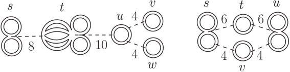
Figure 2: Typical connected Feynman diagrams which contribute to the free energy in the model (5.6).

As in the standard perturbation theory, physical observables such as the free energy are computed by summing all the connected diagrams. Fig.2 shows typical examples of connected diagrams which contribute to the free energy. More precisely, the connected diagrams in this theory are those which are connected by dashed lines or by double lines. One can show that only such diagrams indeed contribute to the calculation of observables.

Since we are interested in the planar limit, we consider what type of diagrams is dominant in this limit. It is easy to see that the leading order in the $1/N$ expansion is given by the diagrams that satisfy two conditions. One is that they are planar diagrams with respect to the double lines in the ordinary sense. The other is that they are divided by two parts by cutting any dashed line. We call the diagrams satisfying the latter condition ‘tree’ diagrams in this paper. We can see that the diagrams in which the dashed lines form any loop (i.e. non-‘tree’ diagrams) give subleading contribution. In Fig.2, the left diagram contributes to the free energy in the large-$N$ limit while the right diagram is suppressed since the dashed lines form a loop.

5.2 Feynman rule for Chern-Simons matrix model

Next, we construct a Feynman rule of CS matrix model (2.17). We first rewrite (2.17) into a manifestly $U(N)$ invariant form as we did for (4.4) in the previous subsection. The identification for the coupling constants shown in (4.6) allows us to put

$$\lambda=g_{s}N,$$ (5.14)

where $\lambda$ is the ’t Hooft coupling in (5.6) which is introduced in (5.2). If we redefine the fields as $\phi_{i}\equiv\beta_{i}/\sqrt{\lambda}$. we can rewrite the measure in (2.17) as follows,

$$\prod_{i<j}\left(2\sinh\frac{\beta_{i}-\beta_{j}}{2}\right) \sim\prod_{i<j}(\phi_{i}-\phi_{j})^{2}\exp\left\{{\sum_{i,j}\log\frac{\sinh\frac{\sqrt{\lambda}}{2}(\phi_{i}-\phi_{j})}{\frac{\sqrt{\lambda}}{2}(\phi_{i}-\phi_{j})}}\right\}$$

$$=\prod_{i<j}(\phi_{i}-\phi_{j})^{2}\exp\left\{\sum_{i,j}\sum_{n=1}^{\infty}\log\left(1+\frac{\lambda}{4\pi^{2}n^{2}}(\phi_{i}-\phi_{j})^{2}\right)\right\}$$

$$=\prod_{i<j}(\phi_{i}-\phi_{j})^{2}\exp\left\{\sum_{i,j}\sum_{k=1}^{\infty}\frac{-\zeta(2k)}{k}\left(\frac{-\lambda}{4\pi^{2}}\right)^{k}\sum_{m=0}^{2k}\left(\begin{array}[]{c}2k\\ m\\ \end{array}\right)\phi_{i}^{m}(-\phi_{j})^{2k-m}\right\},$$ (5.17)

where $\sim$ represents that we have omitted an irrelevant constant factor and $\zeta(z)$ is the zeta function. We have used the formula,

$$\frac{\sinh\pi x}{\pi x}=\prod_{n=1}^{\infty}\left(1+\frac{x^{2}}{n^{2}}\right),$$ (5.18)

to obtain the second line in (5.17). If we introduce an $U(N)$ covariant matrix $\phi$ such that its $i$-th eigenvalue is given by $\phi_{i}$, we obtain the following partition function for CS matrix model on $S^{3}$ [48],

$${\cal Z}_{CSM}\sim\int d\phi\exp\left\{-\frac{N}{2}{\rm tr}\phi^{2}-V(\phi)\right\},$$ (5.19)

where the potential $V(\phi)$ is given by the double trace interaction,

$$V(\phi)=\sum_{k=1}^{\infty}\frac{\zeta(2k)}{k}\left(\frac{-\lambda}{4\pi^{2}}\right)^{k}\sum_{m=0}^{2k}\left(\begin{array}[]{c}2k\\ m\\ \end{array}\right){\rm tr}\phi^{m}{\rm tr}(-\phi)^{2k-m}.$$ (5.22)

We construct the Feynman rule of (5.19) as follows. The tree level propagator is given by

$$\langle\phi_{ij}\phi_{kl}\rangle=\frac{1}{N}\delta_{il}\delta_{jk},$$ (5.23)

which is expressed by double lines as usual in the standard double line notation. The double trace interaction vertices are represented in terms of dashed lines which connect two traces as in the case of (5.6). They are represented in the same way as in Fig.1 except that we do not need the indeces $s,t$ here. Fig.1 (right) without $s,t$ corresponds to the term in (5.22) which includes ${\rm tr}\phi^{6}{\rm tr}\phi^{4}$. The weights of the vertices can be easily read off from (5.22). The ${\rm tr}\phi^{a}{\rm tr}\phi^{b}$ vertex gives a constant factor,

$$-\frac{4\zeta(a+b)}{a+b}\left(\frac{-\lambda}{4\pi^{2}}\right)^{\frac{a+b}{2}}(-1)^{a}\left(\begin{array}[]{c}a+b\\ a\\ \end{array}\right).$$ (5.26)

As in the case of (5.6), connected diagrams in this theory are those which are connected by dashed lines or by double lines. In the $N\rightarrow\infty$ limit, the leading order in the $1/N$ expansion is given by the diagrams which are planar in the ordinary sense and ‘tree’ with respect to dashed lines. For instance, the right diagram in Fig.2 in the case of (5.19) (i.e. the diagram without the indeces $s,t,u,\cdots$.) is suppressed in the large-$N$ limit since the dashed lines form a loop. Note that the Feynman diagrams in (5.19) have the one-to-one correspondence to those in (5.6).

5.3 Equivalence between two theories

In this subsection, we show that (5.6) and (5.19) are equivalent in the limit shown in (4.5) and (4.6). We can prove this equivalence by showing that, in this limit, each Feynman diagram in (5.6) takes the same value as the corresponding diagram in (5.19). Note that we have already imposed the identification of the coupling constants shown in (4.6) through (5.2) and (5.14).

5.3.1 Free energy

In order to prove the equivalence, we first show that

$$\frac{\cal F}{N^{2}(\Lambda+1)}=\frac{{\cal F}_{M}}{N^{2}}$$ (5.27)

holds in the limit shown in (4.5) and (4.6), where ${\cal F}$ and ${\cal F}_{M}$ are the free energies of (5.6) and (5.19), respectively. As an example of the Feynman diagrams contributing to the free energy, let us consider the left diagram in Fig.2 for the both theories. Since the only deference between (5.13) and (5.26) is $\frac{1}{2(s-t)^{a+b}}$ and $\zeta(a+b)$, it is easy to see that the diagram in (5.6) divided by $N^{2}(\Lambda+1)$ becomes equal to the corresponding diagram in (5.19) divided by $N^{2}$ if

$$\frac{1}{2^{4}(\Lambda+1)}\sum_{s=-\Lambda/2}^{\Lambda/2}\sum_{\begin{subarray}{c}t=-\Lambda/2\\ (t\neq s)\end{subarray}}^{\Lambda/2}\sum_{\begin{subarray}{c}u=-\Lambda/2\\ (u\neq t)\end{subarray}}^{\Lambda/2}\sum_{\begin{subarray}{c}v=-\Lambda/2\\ (v\neq u)\end{subarray}}^{\Lambda/2}\sum_{\begin{subarray}{c}w=-\Lambda/2\\ (w\neq u)\end{subarray}}^{\Lambda/2}\frac{1}{(s-t)^{8}(t-u)^{10}(u-v)^{4}(u-w)^{4}}$$

$$=\zeta(8)\zeta(10)\zeta(4)^{2}$$ (5.28)

holds. In fact, this identity holds in the $\Lambda\rightarrow\infty$ limit. We show the proof of (5.28) in appendix B. Thus, we see that the two diagrams with the appropriate normalization shown in (5.27) take the same value in the $\Lambda\rightarrow\infty$ limit.

We can show more general formula which includes (5.28) as a special case. Let us consider generic ‘tree’ planar diagram in (5.6) shown in Fig.3. For this diagram, we can show the following identity in the large-$\Lambda$ limit,

$$\frac{1}{2^{n}(\Lambda+1)}\sum_{\{s_{a}\}}\frac{1}{(s_{1}-s_{2})^{2k_{1}}(s_{1}-s_{3})^{2k_{2}}\cdots(s_{n}-s_{n+1})^{2k_{n}}}=\prod_{a=1}^{n}\zeta(2k_{a}),$$ (5.29)

where $\{s_{a}\}$ represents the set of indeces $(s_{1},\cdots,s_{n+1})$ and each $s_{a}$ runs from $-\Lambda/2$ to $\Lambda/2$. Note that the singular points such as $s_{1}=s_{2}$ are not included in the summations as in the simpler case of (5.28). The proof of (5.29) is shown in appendix B. (5.29) implies that the value of the diagram in Fig.3 divided by $N^{2}(\Lambda+1)$ is equal to the same diagram in (5.19) divided by $N^{2}$. We find, therefore, that (5.27) holds to all orders in $\lambda$ in the limit (4.5).

Figure 3: Generic ‘tree’ planar diagram in (5.6). Each blob represents a planar diagram.

We can check (5.27) also by performing an explicit perturbative calculation. The detail of the calculation is shown in appendix C. Up to ${\cal O}(\lambda^{3})$, the result is given by,

$$\frac{\cal F}{N^{2}(\Lambda+1)}= \frac{\lambda}{12}+\frac{\lambda^{2}}{288}+\frac{\lambda^{2}}{1440N^{2}}$$

$$+\frac{\lambda^{3}}{N^{2}}\left(\frac{1}{9072}+\frac{1}{48\pi^{6}\Lambda}\sum_{s,t,u}\frac{1}{(s-t)^{2}(t-u)^{2}(u-s)^{2}}\right)+{\cal O}(\lambda^{4}),$$ (5.30)

while for CS matrix model, we can read off the counterpart from (2.24) as,

$$\frac{{\cal F}_{M}}{N^{2}}=\frac{\lambda}{12}-\frac{\lambda}{12N^{2}}+\frac{\lambda^{2}}{288}+\frac{\lambda^{2}}{96N^{2}}+{\cal O}(\lambda^{4}).$$ (5.31)

Thus, we see that if one takes the limit shown in (4.5) and (4.6), (5.30) indeed agrees with (5.31).

5.3.2 Unknot Wilson loop

In terms of the formula (5.29), we can show that other physical observables also take the same values in the two theories. In the following, we show that the VEV of unknot Wilson loop in CS theory which is given by (2.23) is also reproduced from the model (4.4).

We introduce the Wilson loop operator in ${\cal N}=1^{*}$ matrix model proposed in [34],

$$\hat{W}({\cal K})=\frac{1}{M}{\rm Tr}\left[P\exp\left(i\mu\int^{1}_{0}X_{i}E^{i}_{M}(z(\sigma))\frac{dz^{M}(\sigma)}{d\sigma}d\sigma\right)\right],$$ (5.32)

where $z^{M}$ are coordinates on $S^{3}$, $\sigma$ parameterize the knot ${\cal K}$ and $E^{i}_{M}dz^{M}$ are the right-invariant 1-forms on $S^{3}$ defined in (A.4). In [34], it is shown through Taylor’s T-duality that this operator is reduced to the Wilson loop operator on $S^{3}$ in the continuum limit. In order to see the correspondence to the unknot Wilson loop in CS theory, we consider (5.32) with an unknot contour. We take the simplest one, a great circle on $S^{3}$, as such contour. The great circle is parameterized, for example, by

$$(\theta,\varphi,\psi)=\left(\frac{\pi}{2},0,4\pi\sigma\right),$$ (5.33)

with $\sigma\in(0,1]$. By substituting (5.33) into (5.32) and setting $\mu=1$, we obtain,

$$\hat{W}({\rm unknot})=\frac{1}{M}{\rm Tr}\left(e^{4\pi iX_{3}}\right).$$ (5.34)

As in section 3.3, we take the gauge in which $X_{3}=\Phi$ is diagonalized. Recall that after we integrate out the delta functions shown in (3.19) which appear in the partition function, the remaining eigenvalues of $\Phi$ are represented by $y_{si}/2$. Then, in (5.34), if we make the analytic continuation $y_{si}\rightarrow-iy_{si}$ and the field redefinition $y_{si}=\sqrt{\lambda}\phi_{si}/{2\pi}$, we obtain,

$$\hat{W}({\rm unknot})=\frac{\Omega}{M}\sum_{s,i}e^{\sqrt{\lambda}\phi_{si}}=\frac{1}{N(\Lambda+1)}\sum_{s}{\rm Tr}e^{\sqrt{\lambda}\phi_{s}}.$$ (5.35)

Therefore, we find that the unknot Wilson loop operator in the fundamental representation is given by (5.35) in (4.4).

On the other hand, in CS matrix model (2.17), the VEV of unknot Wilson loop is given by (2.22). Then, the equivalence for the unknot Wilson loop is expressed in terms of $\phi$ and $\phi_{s}$ as

$$\frac{1}{N(\Lambda+1)}\sum_{s}\langle{\rm Tr}e^{\sqrt{\lambda}\phi_{s}}\rangle=\frac{1}{N}\langle{\rm Tr}e^{\sqrt{\lambda}\phi}\rangle_{M},$$ (5.36)

where $\langle\cdots\rangle$ and $\langle\cdots\rangle_{M}$ denote the expectation values in (5.6) and (5.19), respectively. We can show (5.36) in all orders in perturbation theory. In perturbation theory, the VEVs in (5.36) are calculated by expanding the exponentials. Then, (5.36) is satisfied if

$$\frac{1}{\Lambda+1}\sum_{s}\langle{\rm Tr}\phi^{n}_{s}\rangle=\langle{\rm Tr}\phi^{n}\rangle_{M}$$ (5.37)

holds for $n=0,1,2,\cdots$. Because (5.29) holds for all the ‘tree’ planar Feynman diagrams contributing to the VEVs in (5.37), we find that (5.37) and hence (5.36) hold in all orders in $\lambda$. Thus, we have shown that the VEV of unknot Wilson loop in CS theory is reproduced from the reduced model.

It is straightforward to check (5.36) explicitly by calculating the VEV of (5.35) in perturbation theory. The method of calculating the VEV is almost the same as in the case of the free energy. We show the detail of this calculation in appendix C. In the large-$\Lambda$ limit, the result is given by

$$\frac{1}{N(\Lambda+1)}\sum_{s}\langle{\rm Tr}e^{\sqrt{\lambda}\phi_{s}}\rangle=1+\frac{\lambda}{2}+\frac{\lambda^{2}}{6}+\frac{\lambda^{2}}{24N^{2}}+\frac{\lambda^{3}}{24}+\frac{7\lambda^{3}}{240N^{2}}+{\cal O}(\lambda^{4}).$$ (5.38)

On the other hand, (2.23) is expanded as,

$$\langle W_{\square}({\rm unknot})\rangle_{CS} =1+\frac{\lambda}{2}+\frac{\lambda^{2}}{6}-\frac{\lambda^{2}}{24N^{2}}+\frac{\lambda^{3}}{24}-\frac{\lambda^{3}}{48N^{2}}+{\cal O}(\lambda^{4}).$$ (5.39)

Comparing (5.38) and (5.39), we can see that (5.36) indeed holds in the $N\rightarrow\infty$ limit.

5.4 Extension to $S^{3}/Z_{q}$

We can show the similar equivalence for the case of CS theory on $S^{3}/Z_{k}$. Although this theory possesses many nontrivial vacua, we consider the trivial vacuum only in this paper.

The vacua in CS theory on $S^{3}/Z_{q}$ are characterized by the holonomy along the circle on which $Z_{q}$ acts. In [48], it is shown that the partition function of CS theory on $S^{3}/Z_{q}$ for each vacuum sector is reduced to the partition function of a matrix model similar to (5.19). For example, the partition function for the trivial vacuum sector is given by (5.19) with $\lambda$ replaced by $\lambda^{\prime}\equiv g_{s}N/q$.

On the other hand, as mentioned in the last part in section 4, the statistical model for CS theory on $S^{3}/Z_{q}$ is given by replacing $s,t$ in (4.4) with $qs,qt$. By following the same calculation as (5.1) and (5.5), we can see that such model is equivalent to (5.6) with $\lambda$ replaced by $\lambda^{\prime\prime}\equiv 2\pi^{2}g^{2}N/q^{2}$.

Then, with the identification $\lambda^{\prime}=\lambda^{\prime\prime}$, we see that the two theories are equivalent in the limit (4.5). Thus, we find that the theory on $S^{3}/Z_{q}$ is also reproduced from the matrix model.

6 Monte Carlo simulation

The large-$N$ equivalence between (4.4) and CS theory on $S^{3}$ can be understood also from the agreement of the eigenvalue densities in the two theories. In this section, by performing a Monte Carlo simulation, we show that the eigenvalue density of $y_{si}$ at the saddle point of (4.4) coincides with that of $\beta_{i}$ in (2.17) if $|s|$ is sufficiently small compared to the cutoff $\Lambda/2$. The eigenvalue densities for $y_{si}$ with $s$ near the cutoff have some deviation from the density of $\beta_{i}$. However, we will see that such cutoff effect vanishes in the continuum limit and does not contribute to values of physical observables. From this property of the eigenvalue density, we can also give another check of the equivalences for free energy and unknot Wilson loop operator which we have shown in the previous section.

Let us introduce the eigenvalue density of $\beta_{i}$ in CS theory on $S^{3}$ as,

$$\rho(x)=\frac{1}{N}\sum_{i=1}^{N}\delta(x-\beta_{i}/(2\pi)),$$ (6.1)

and the eigenvalue density of $y_{si}$ in (4.4) as,

$$\rho^{(s)}(x)=\frac{1}{N}\sum_{i=1}^{N}\delta(x-y_{si}).$$ (6.2)

We also define the difference between (6.1) and (6.2) as,

$$\Delta\rho^{(s)}(x)=\rho^{(s)}(x)-\rho(x).$$ (6.3)

By performing a Monte Carlo simulation of (4.4), we can see that $\Delta\rho^{(s)}(x)=0$ for $s\sim{\cal O}(1)$ while $\Delta\rho^{(s)}(x)\neq 0$ if $s$ is near the cutoff $\pm\Lambda/2$. Figure 4 shows the result of the simulation. This result shows that as one goes toward the midpoint $s=0$, the distribution converges rapidly to the distribution of CS theory on $S^{3}$. From this result, we conclude that the deviation of the eigenvalue density exists only for sufficiently large $|s|$.

Figure 4: The eigenvalue distribution of $y_{si}$ in our model is plotted for $s=0,28,32,36,40$ with $\lambda=0.25$, $\Lambda=80$ and $N=48$. The dashed line represents the distribution $\rho(x)$ in CS theory on $S^{3}$. The error bars are omitted since they are smaller than the symbol size

We have also verified through the Monte Carlo simulation that $\Delta\rho^{(s)}(x)$ possesses the following property,

$$\lim_{\Lambda\rightarrow\infty}\frac{1}{\Lambda+1}\int dx\sum_{s=-\Lambda/2}^{\Lambda/2}|\Delta\rho^{(s)}(x)|=0.$$ (6.4)

This fact is shown as follows. Let us consider the saddle point equation of (4.4),

$$\frac{2}{g^{2}}x-\int dx^{\prime}\sum_{t=-\Lambda/2}^{\Lambda/2}\rho^{(t)}(x^{\prime})\left\{\frac{1}{x-x^{\prime}+i(s-t)}+\frac{1}{x-x^{\prime}-i(s-t)}\right\}=0.$$ (6.5)

Because $\Delta\rho^{(s)}(x)=0$ for $s\sim{\cal O}(1)$, in order for (6.5) to be satisfied, $\Delta\rho^{(s)}(x)$ with $s$ near the cutoff should behave as

$$\Delta\rho^{(s)}(x)\sim\frac{1}{\Lambda/2-|s|}.$$ (6.6)

Then, we can expect that

$$\frac{1}{\Lambda+1}\int dx\sum_{s=-\Lambda/2}^{\Lambda/2}|\Delta\rho^{(s)}(x)|\sim\frac{\log\Lambda}{\Lambda},$$ (6.7)

in the limit $\Lambda\rightarrow\infty$ so that (6.4) is satisfied. We confirmed (6.7) through the Monte Carlo simulation. Figure 5 is the result of the simulation and it shows that the quantity on the left hand side in (6.7) is indeed nicely fitted by $f(x)=a+b\frac{\log\Lambda}{\Lambda}$ with $a\simeq 0$.

Figure 5: $\frac{1}{\Lambda+1}\int dx\sum_{s=-\Lambda/2}^{\Lambda/2}|\Delta\rho^{(s)}(x)|$ is plotted against $\log\Lambda/\Lambda$. $\lambda=0.25$ and $N$ has already been extrapolated from $N=24,32,48$ to $N=\infty$ by a linear function of $1/N^{2}$. The dotted line represents the extrapolation of the plots using $f(x)=a+b\frac{\log\Lambda}{\Lambda}$ with $a$ and $b$ constants. The error bars are smaller than the symbol size.

If we assume (6.4) or (6.7), we check that the equivalence of the free energy (5.27) indeed holds. Free energy of (4.4) is written in terms of (6.2) as,

$$\frac{{\cal F}}{\Lambda N^{2}}=-\frac{1}{g^{2}\Lambda}\sum_{s}\int dxx^{2}\rho^{(s)}(x)+\frac{1}{2\Lambda}\sum_{s\neq t}\int dxdx^{\prime}\rho^{(s)}(x)\log\{(x-x^{\prime})^{2}+(s-t)^{2}\}\rho^{(t)}(x^{\prime}).$$ (6.8)

Then, by substituting (6.3), we obtain

$$\frac{{\cal F}}{\Lambda N^{2}} =-\frac{1}{g^{2}}\int dxx^{2}\rho(x)+\frac{1}{2\Lambda}\sum_{s\neq t}\int dxdx^{\prime}\rho(x)\log\{(x-x^{\prime})^{2}+(s-t)^{2}\}\rho(x^{\prime})$$

$$\;\;-\frac{1}{g^{2}\Lambda}\sum_{s}\int dxx^{2}\Delta\rho^{(s)}(x)+\frac{1}{\Lambda}\sum_{s\neq t}\int dxdx^{\prime}\rho(x)\log\{(x-x^{\prime})^{2}+(s-t)^{2}\}\Delta\rho^{(t)}(x^{\prime})$$

$$\;\;+\frac{1}{2\Lambda}\sum_{s\neq t}\int dxdx^{\prime}\Delta\rho^{(s)}(x)\log\{(x-x^{\prime})^{2}+(s-t)^{2}\}\Delta\rho^{(t)}(x^{\prime}).$$ (6.9)

By using the formula (5.18), we can show that the first line on the right hand side of (6.9) is equal to ${\cal F}_{M}/N^{2}$ in CS matrix model in the limit $\Lambda\rightarrow\infty$. We can further show that the second and the third lines vanish in $\Lambda\rightarrow\infty$ as follows. Let us introduce a sufficiently large but finite constant $b$ such that the eigenvalue densities for all $s$ fit in the interval $[-b,b]$. Such $b$ exists because the attractive force in (6.5) coming from the Gaussian potential is stronger than the repulsive force for $|x|\gg 1$ so that $\rho^{(s)}(x)$ has a compact support. Then, the first term in the second line is bounded as

$$-\frac{1}{g^{2}\Lambda}\sum_{s=-\Lambda/2}^{\Lambda/2}\int dxx^{2}\Delta\rho^{(s)}(x)\leq\frac{b^{2}}{g^{2}\Lambda}\int dx\sum_{s=-\Lambda/2}^{\Lambda/2}|\Delta\rho^{(s)}(x)|,$$ (6.10)

Because of (6.4), we find that this term does not contribute to ${\cal F}/(\Lambda N^{2})$ in the $\Lambda\rightarrow\infty$ limit. We can apply the same argument to all the terms in the second and the third lines in (6.9). Thus, we have given another check of (5.27).

We can also show the equivalence for unknot Wilson loop operator. Since the VEV in (4.4) can be written as

$$\langle\hat{W}({\rm unknot})\rangle=\frac{\Omega}{M}\langle\sum_{s,i}e^{2\pi y_{si}}\rangle=\frac{1}{N(\Lambda+1)}\int dx\sum_{s}\langle\rho^{(s)}(x)\rangle e^{2\pi x},$$ (6.11)

Using (6.4), we find that

$$\langle\hat{W}({\rm unknot})\rangle\rightarrow\frac{1}{N}\int dx\langle\rho(x)\rangle e^{2\pi x}=\langle W_{\square}({\rm unknot})\rangle_{CS},$$ (6.12)

in the limit $\Lambda\rightarrow\infty$. Thus, we have given another derivation of the equivalence for unknot Wilson loop.

7 Conclusion and discussion

In this paper, we studied a matrix model that is obtained by the dimensional reduction of CS theory on $S^{3}$ to zero dimension. We found that expanded around the particular background corresponding to $S^{3}$, it reproduces the original theory on $S^{3}$ in the planar limit. We calculated the partition function and the VEV of the Wilson loop in the theory around the background of the matrix model and verified that they agree with those in the planar CS theory on $S^{3}$. We checked these results also by performing the Monte Carlo simulation. We also extended this equivalence to the case of CS theory on $S^{3}/Z_{q}$.

In this paper, we only consider the unknot Wilson loop. It is relevant to see whether the VEV of the Wilson loop for a real knot is reproduced in our formulation. We should verify that the VEV of the Wilson loops does not change against continuous deformation of the loops, such that it indeed represents a topological invariant. We should also extend our analysis to the case of the Wilson loop with general representation ${\cal R}$ of $SU(N)$. It is also interesting to see whether we can use our formulation to achieve the large-$N$ reduction for other theories including the CS term such as the ABJM model[49].

Appendix A $S^{3}$ and $S^{2}$

In this appendix, we summarize some useful facts about $S^{3}$ and $S^{2}$ (See also [15, 12]). $S^{3}$ is viewed as the $SU(2)$ group manifold. We parameterize an element of $SU(2)$ in terms of the Euler angles as

$$g=e^{-i\varphi\sigma_{3}/2}e^{-i\theta\sigma_{2}/2}e^{-i\psi\sigma_{3}/2},$$ (A.1)

where $0\leq\theta\leq\pi$, $0\leq\varphi<2\pi$, $0\leq\psi<4\pi$. The periodicity with respect to these angle variables is expressed as

$$(\theta,\varphi,\psi)\sim(\theta,\varphi+2\pi,\psi+2\pi)\sim(\theta,\varphi,\psi+4\pi).$$ (A.2)

The isometry of $S^{3}$ is $SO(4)=SU(2)\times SU(2)$, and these two $SU(2)$’s act on $g$ from left and right, respectively. We construct the right-invariant 1-forms,

$$dgg^{-1}=-i\mu E^{i}\sigma_{i}/2,$$ (A.3)

where $E^{i}$ are explicitly given by

$$E^{1}=\frac{1}{\mu}(-\sin\varphi d\theta+\sin\theta\cos\varphi d\psi),$$

$$E^{2}=\frac{1}{\mu}(\cos\varphi d\theta+\sin\theta\sin\varphi d\psi),$$

$$E^{3}=\frac{1}{\mu}(d\varphi+\cos\theta d\psi).$$ (A.4)

The radius of $S^{3}$ is $2/\mu$. $E_{i}$ satisfy the Maurer-Cartan equation

$$dE^{i}-\frac{\mu}{2}\epsilon_{ijk}E^{j}\wedge E^{k}=0.$$ (A.5)

The metric is constructed from $E^{i}$ as

$$ds^{2}=E^{i}E^{i}=\frac{1}{\mu^{2}}\left(d\theta^{2}+\sin^{2}\theta d\varphi^{2}+(d\psi+\cos\theta d\varphi)^{2}\right).$$ (A.6)

The Killing vector dual to $E^{i}$ is given by

$${\cal{L}}_{i}=-\frac{i}{\mu}E^{M}_{i}\partial_{M},$$ (A.7)

where $M=\theta,\varphi,\psi$ and $E^{M}_{i}$ are inverse of $E^{i}_{M}$. The Killing vector is explicitly expressed as

$${\cal{L}}_{1}=-i\left(-\sin\varphi\partial_{\theta}-\cot\theta\cos\varphi\partial_{\varphi}+\frac{\cos\varphi}{\sin\theta}\partial_{\psi}\right),$$

$${\cal{L}}_{2}=-i\left(\cos\varphi\partial_{\theta}-\cot\theta\sin\varphi\partial_{\varphi}+\frac{\sin\varphi}{\sin\theta}\partial_{\psi}\right),$$

$${\cal{L}}_{3}=-i\partial_{\varphi}.$$ (A.8)

From the Maurer-Cartan equation (A.5), one can show that the Killing vector satisfies the $SU(2)$ algebra $[{\cal{L}}_{i},{\cal{L}}_{j}]=i\epsilon_{ijk}{\cal{L}}_{k}$.

Next, let us regard $S^{3}$ as a $U(1)$ bundle over $S^{2}=SU(2)/U(1)$. $S^{2}$ is parametrized by $\theta$ and $\varphi$ and covered with two local patches: the patch I defined by $0\leq\theta<\pi$ and the patch II defined by $0<\theta\leq\pi$. In the following, the upper sign represents the patch I while the lower sign represents the patch II. The element of $SU(2)$ in (A.1) is decomposed as

$$g=L\cdot h$$ (A.9)

with

$$L=e^{-i\varphi\sigma_{3}/2}e^{-i\theta\sigma_{2}/2}e^{\pm i\varphi\sigma_{3}/2},$$

$$h=e^{-i(\psi\pm\varphi)\sigma_{3}/2}.$$ (A.10)

$L$ represents an element of $S^{2}$, while $h$ represents the fiber $U(1)$. The fiber direction is parametrized by $y=\psi\pm\varphi$. The zweibein of $S^{2}$ is given by the $i=1,2$ components of the left-invariant 1-form, $-iL^{-1}dL=\mu e^{i}\sigma_{i}/2$, which takes the form

$$e^{1}=\frac{1}{\mu}(\pm\sin\varphi d\theta+\sin\theta\cos\varphi d\varphi),$$

$$e^{2}=\frac{1}{\mu}(-\cos\varphi d\theta\pm\sin\theta\sin\varphi d\varphi).$$ (A.11)

This zweibein gives the standard metric of $S^{2}$ with the radius $1/\mu$:

$$ds^{2}=e^{i}e^{i}=\frac{1}{\mu^{2}}(d\theta^{2}+\sin^{2}\theta d\varphi^{2}).$$ (A.12)

Making a replacement $\partial_{y}\rightarrow-iq$ in (A.8) leads to the angular momentum operator in the presence of a monopole with magnetic charge $q$ at the origin [50]:

$$L_{1}^{(q)}=i(\sin\varphi\partial_{\theta}+\cot\theta\cos\varphi\partial_{\varphi})-q\frac{1\mp\cos\theta}{\sin\theta}\cos\varphi,$$

$$L_{2}^{(q)}=i(-\cos\varphi\partial_{\theta}+\cot\theta\sin\varphi\partial_{\varphi})-q\frac{1\mp\cos\theta}{\sin\theta}\sin\varphi,$$

$$L_{3}^{(q)}=-i\partial_{\varphi}\mp q,$$ (A.13)

where $q$ is quantized as $q=0,\pm\frac{1}{2},\pm 1,\pm\frac{3}{2},\cdots$, because $y$ is a periodic variable with the period $4\pi$. These operators act on the local sections on $S^{2}$ and satisfy the $SU(2)$ algebra $[L_{i}^{(q)},L_{j}^{(q)}]=i\epsilon_{ijk}L_{k}^{(q)}$. When $q=0$, these operators are reduced to the ordinary angular momentum operators on $S^{2}$ (or $R^{3})$, $L_{i}\equiv L_{i}^{(0)}$. The $SU(2)$ acting on $g$ from left survives as the isometry of $S^{2}$.

Appendix B Proof of equation (5.29)

General ‘tree’ planar diagram shown in Fig.3 consists of several parts (blobs) which are connected by the dashed lines and each part represents a planar diagram. For each part, we define a certain quantity in order to show (5.29). For instance, if we consider the left diagram shown in Fig.2, we define the following quantity for the part labeled by $s$,

$$Q_{s}=\sum_{\begin{subarray}{c}t=-\Lambda/2\\ (t\neq s)\end{subarray}}^{\Lambda/2}\sum_{\begin{subarray}{c}u=-\Lambda/2\\ (u\neq t)\end{subarray}}^{\Lambda/2}\sum_{\begin{subarray}{c}v=-\Lambda/2\\ (v\neq u)\end{subarray}}^{\Lambda/2}\sum_{\begin{subarray}{c}w=-\Lambda/2\\ (w\neq u)\end{subarray}}^{\Lambda/2}\frac{1}{(s-t)^{8}}\frac{1}{(t-u)^{10}}\frac{1}{(u-v)^{4}}\frac{1}{(u-w)^{4}}.$$ (B.1)

Namely, for a dashed line connecting $s$ and $t$, we assign $\frac{1}{(s-t)^{2l}}$ where $2l$ is the number of fields contained in the vertex and $Q_{s}$ is the summation of the product of them with respect to the variables other than $s$. Then, we can see that $Q_{s}$ has a finite value and bounded from above by a certain constant. This is shown as follows. First, note the following identity,

$$\sum_{\begin{subarray}{c}t=-\Lambda/2\\ (t\neq s)\end{subarray}}^{\Lambda/2}\frac{1}{(s-t)^{2l}}=2\zeta(2l)-\zeta(2l,\Lambda/2+s+1)-\zeta(2l,\Lambda/2-s+1),$$ (B.2)

where $\zeta(z)$ and $\zeta(z,a)$ are the zeta function and the generalized zeta function, respectively. They are defined by,

$$\zeta(z)=\sum_{n=1}^{\infty}\frac{1}{n^{z}},\;\;\;\;\zeta(z,a)=\sum_{n=0}^{\infty}\frac{1}{(n+a)^{z}}.$$ (B.3)

Because $\zeta(2l,\Lambda/2+s+1)+\zeta(2l,\Lambda/2-s+1)>0$,

$$Q_{s} <\sum_{\begin{subarray}{c}t=-\Lambda/2\\ (t\neq s)\end{subarray}}^{\Lambda/2}\sum_{\begin{subarray}{c}u=-\Lambda/2\\ (u\neq t)\end{subarray}}^{\Lambda/2}\sum_{\begin{subarray}{c}v=-\Lambda/2\\ (v\neq u)\end{subarray}}^{\Lambda/2}\frac{1}{(s-t)^{8}}\frac{1}{(t-u)^{10}}\frac{1}{(u-v)^{4}}\times 2\zeta(4)$$

$$<\sum_{\begin{subarray}{c}t=-\Lambda/2\\ (t\neq s)\end{subarray}}^{\Lambda/2}\sum_{\begin{subarray}{c}u=-\Lambda/2\\ (u\neq t)\end{subarray}}^{\Lambda/2}\frac{1}{(s-t)^{8}}\frac{1}{(t-u)^{10}}\times 2^{2}\zeta(4)^{2}$$

$$<\sum_{\begin{subarray}{c}t=-\Lambda/2\\ (t\neq s)\end{subarray}}^{\Lambda/2}\frac{1}{(s-t)^{8}}\times 2^{3}\zeta(4)^{2}\zeta(10)$$

$$<2^{4}\zeta(4)^{2}\zeta(8)\zeta(10).$$ (B.4)

Thus, we find that $Q_{s}$ is finite even if we take the limit $\Lambda\rightarrow\infty$. We are able to define $Q_{s}$ also for more general diagram shown in Fig.3. If the diagram is ‘tree’, through the same calculation just as we described above, we see that $Q_{s}$ is bounded from above by a $\Lambda$-independent constant which is given by a product of the zeta functions.

Figure 6: The rectangular box represents a Feynman diagram with ‘tree’-like structure, namely, a diagram which does not contain any loop formed by dashed lines. The circular blob represents a planar diagram which does not include dashed lines.

Then, let us consider the diagram in Fig.6. We can define $Q_{s}$ for this diagram. We assume that the rectangular part in Fig.6 represents a ‘tree’ diagram so that $Q_{s}$ for this diagram is bounded from above. We consider the following quantity,

$$\frac{1}{\Lambda+1}\sum_{s=-\Lambda/2}^{\Lambda/2}\sum_{\begin{subarray}{c}t=-\Lambda/2\\ (t\neq s)\end{subarray}}^{\Lambda/2}\frac{1}{(s-t)^{2l}}Q_{s}=\frac{2}{\Lambda+1}\sum_{s=-\Lambda/2}^{\Lambda/2}(\zeta(2l)-\zeta(2l,\Lambda/2+s+1))Q_{s}.$$ (B.5)

Since there exists a positive $\Lambda$-independent constant $c$ such that $Q_{s}<c$, the second term on the right hand side in (B.5) is bounded as follows,

$$\frac{1}{\Lambda+1}\sum_{s=-\Lambda/2}^{\Lambda/2}\zeta(2l,\Lambda/2+s+1)Q_{s} <\frac{c}{\Lambda+1}\sum_{s=-\Lambda/2}^{\Lambda/2}\zeta(2l,\Lambda/2+s+1)$$

$$=\frac{2c}{\Lambda+1}\sum_{n=1}^{\Lambda+1}\frac{1}{n^{2l-1}}+2c\sum_{n=\Lambda+1}^{\infty}\frac{1}{n^{2l}},$$ (B.6)

where we have used (B.3) to obtain the second line. Because the second line in (B.6) is ${\cal O}(\log\Lambda/\Lambda)$ for $l=1$ and ${\cal O}(1/\Lambda)$ for $l>1$, this quantity goes to zero in the limit $\Lambda\rightarrow\infty$. Therefore, we find from (B.5) and (B.6) that

$$\lim_{\Lambda\rightarrow\infty}\frac{1}{\Lambda+1}\sum_{s=-\Lambda/2}^{\Lambda/2}\sum_{\begin{subarray}{c}t=-\Lambda/2\\ (t\neq s)\end{subarray}}^{\Lambda/2}\frac{1}{(s-t)^{2l}}Q_{s}=\lim_{\Lambda\rightarrow\infty}\frac{2\zeta(2l)}{\Lambda+1}\sum_{s=-\Lambda/2}^{\Lambda/2}Q_{s}.$$ (B.7)

Then, for instance, we can show the following equality by using (B.7) iteratively,

$$\lim_{\Lambda\rightarrow\infty}\frac{1}{\Lambda+1}\sum_{s=-\Lambda/2}^{\Lambda/2}\sum_{\begin{subarray}{c}t=-\Lambda/2\\ (t\neq s)\end{subarray}}^{\Lambda/2}\sum_{\begin{subarray}{c}u=-\Lambda/2\\ (u\neq t)\end{subarray}}^{\Lambda/2}\sum_{\begin{subarray}{c}v=-\Lambda/2\\ (v\neq u)\end{subarray}}^{\Lambda/2}\sum_{\begin{subarray}{c}w=-\Lambda/2\\ (w\neq u)\end{subarray}}^{\Lambda/2}\frac{1}{(s-t)^{8}}\frac{1}{(t-u)^{10}}\frac{1}{(u-v)^{4}}\frac{1}{(u-w)^{4}}$$

$$=\lim_{\Lambda\rightarrow\infty}\frac{1}{\Lambda+1}\sum_{s=-\Lambda/2}^{\Lambda/2}\sum_{\begin{subarray}{c}t=-\Lambda/2\\ (t\neq s)\end{subarray}}^{\Lambda/2}\sum_{\begin{subarray}{c}u=-\Lambda/2\\ (u\neq t)\end{subarray}}^{\Lambda/2}\sum_{\begin{subarray}{c}v=-\Lambda/2\\ (v\neq u)\end{subarray}}^{\Lambda/2}\frac{1}{(s-t)^{8}}\frac{1}{(t-u)^{10}}\frac{1}{(u-v)^{4}}\times 2\zeta(4)$$

$$=\lim_{\Lambda\rightarrow\infty}\frac{1}{\Lambda+1}\sum_{s=-\Lambda/2}^{\Lambda/2}\sum_{\begin{subarray}{c}t=-\Lambda/2\\ (t\neq s)\end{subarray}}^{\Lambda/2}\sum_{\begin{subarray}{c}u=-\Lambda/2\\ (u\neq t)\end{subarray}}^{\Lambda/2}\frac{1}{(s-t)^{8}}\frac{1}{(t-u)^{10}}\times 2^{2}\zeta(4)^{2}$$

$$\;\;\;\vdots$$

$$=\lim_{\Lambda\rightarrow\infty}\frac{1}{\Lambda+1}\sum_{s=-\Lambda/2}^{\Lambda/2}2^{4}\zeta(4)^{2}\zeta(8)\zeta(10)$$

$$=2^{4}\zeta(4)^{2}\zeta(8)\zeta(10).$$ (B.8)

This is nothing but (5.28). Since (B.8) implies that we can replace $\sum_{s=-\Lambda/2}^{\Lambda/2}1/(s-t)^{2l}$ on the tip of a branch in the ‘tree’ diagrams with $\zeta(2l)$ in the $\Lambda\rightarrow\infty$ limit, applying the same calculation, we can show (5.29) for the generic ‘tree’ planar diagram shown in Fig.3.

Appendix C Perturbative calculation

In this appendix, we explicitly evaluate the free energy of (5.6) and the VEV of (5.35) up to $\mathcal{O}(\lambda^{3})$. We perform the usual perturbation theory in (5.6).

First, we will calculate the free energy. Let us expand the interaction terms in terms of the power of the coupling

$$\tilde{V}(\phi_{s}) =\sum_{k=1}^{\infty}\tilde{V}_{k}(\phi_{s}),$$

$$\tilde{V}_{k}(\phi_{s}) \equiv\sum_{s\neq t}\frac{1}{2k(s-t)^{2k}}\left(\frac{-\lambda}{4\pi^{2}}\right)^{k}\sum_{m=0}^{2k}{}_{2k}C_{m}{\rm tr}\phi_{s}^{m}{\rm tr}(-\phi_{t})^{2k-m},$$ (C.1)

and the partition function as

$$\mathcal{Z}=\sum_{k=0}^{\infty}\mathcal{Z}_{k},$$ (C.2)

where $\mathcal{Z}_{k}$ is the part of which the coupling dependence is $\mathcal{O}(\lambda^{k})$. $\mathcal{Z}_{0}$ is the free part,

$$\mathcal{Z}_{0}=\int\prod_{s}d\phi_{s}e^{-\frac{N}{2}\sum_{s}\mbox{tr}\phi_{s}^{2}}=\left(\frac{2\pi}{N}\right)^{N^{2}(\Lambda+1)/2},$$ (C.3)

and $\mathcal{Z}_{k}\;(k=1,2,3)$ are given by

$$\frac{\mathcal{Z}_{1}}{{\cal Z}_{0}} =-\langle\tilde{V}_{1}\rangle,$$

$$\frac{\mathcal{Z}_{2}}{{\cal Z}_{0}} =-\langle\tilde{V}_{2}\rangle+\frac{1}{2}\langle\tilde{V_{1}}^{2}\rangle,$$

$$\frac{\mathcal{Z}_{3}}{{\cal Z}_{0}} =-\langle\tilde{V}_{3}\rangle+\langle\tilde{V_{2}}\tilde{V_{1}}\rangle-\frac{1}{3!}\langle\tilde{V_{1}}^{3}\rangle.$$ (C.4)

We define the free energy of our matrix model as

$$\mathcal{F} =\ln\frac{\mathcal{Z}}{\mathcal{Z}_{0}}$$

$$=\ln\left(1+\frac{{\cal Z}_{1}}{{\cal Z}_{0}}+\frac{{\cal Z}_{2}}{{\cal Z}_{0}}+\frac{{\cal Z}_{3}}{{\cal Z}_{0}}+\cdots\right).$$ (C.5)

Substituting (C.4) into (C.5), we obtain

$$\mathcal{F}=-\langle\tilde{V}_{1}\rangle_{c}-\langle\tilde{V}_{2}\rangle_{c}+\frac{1}{2}\langle\tilde{V_{1}}^{2}\rangle_{c}-\langle\tilde{V}_{3}\rangle_{c}+\langle\tilde{V_{2}}\tilde{V_{1}}\rangle_{c}-\frac{1}{3!}\langle\tilde{V_{1}}^{3}\rangle_{c}+\cdots,$$ (C.6)

where $\langle\cdots\rangle_{c}$ means the connected part of $\langle\cdots\rangle$. For example, $\langle\tilde{V}_{1}^{2}\rangle_{c}$ is calculated as follows;

$$\frac{1}{2}\langle\tilde{V_{1}}^{2}\rangle_{c} =\frac{1}{2}\biggl{(}4\sum_{s,t,u}\frac{1}{2(s-t)^{2}\cdot 2(t-u)^{2}}\left(\frac{\lambda}{4\pi^{2}}\right)^{2}N^{2}\langle\mbox{tr}\phi^{2}\mbox{tr}\phi^{2}\rangle_{c}$$

$$\qquad+2\sum_{s,t}\frac{1}{2(s-t)^{2}\cdot 2(t-s)^{2}}\left(\frac{\lambda}{4\pi^{2}}\right)^{2}2^{2}\langle\mbox{tr}\phi\mbox{tr}\phi\rangle_{c}^{2}\biggr{)}$$

$$=\frac{\lambda^{2}}{4\pi^{4}}N^{2}(\Lambda+1)\zeta(2)^{2}+\frac{\lambda^{2}}{8\pi^{4}}(\Lambda+1)\zeta(4)$$

$$=(\Lambda+1)\left(N^{2}\frac{\lambda^{2}}{144}+\frac{\lambda^{2}}{720}\right).$$ (C.7)

In Feynman diagram introduced in subsection 5.1, one can describe this contribution as Fig. 7.

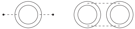
Figure 7: Feynman diagrams corresponding to (C.7). The left is planar diagram ($\mathcal{O}(N^{2})$), while the right is nonplanar ($\mathcal{O}(1)$).

Performing the similar calculations, we finally obtain (5.30).

Second, we perform a perturbative calculation of the VEV of the unknot Wilson loop (5.35) up to $\mathcal{O}(\lambda^{3})$. We expand the VEV as

$$\frac{1}{(\Lambda+1)N}\sum_{s}\langle\mathop{\rm Tr}e^{\sqrt{\lambda}\phi_{s}}\rangle =\frac{1}{(\Lambda+1)N}\sum_{l=0}^{\infty}\frac{\lambda^{l/2}}{l!}\sum_{s}\langle\mbox{tr}(\phi_{s})^{l}\rangle$$

$$=1+\frac{1}{(\Lambda+1)N}\sum_{l=1}^{\infty}\frac{\lambda^{l}}{(2l)!}\sum_{s}(\langle\mbox{tr}(\phi_{s})^{2l}\rangle_{0}+\langle\mbox{tr}(\phi_{s})^{2l}\rangle_{int}),$$ (C.8)

where $\langle\cdots\rangle_{0}$ means the ladder part and $\langle\cdots\rangle_{int}$ means to evaluate with interaction vertices. The ladder part is easily calculated as follows

$$\sum_{s}\langle\mbox{tr}\phi_{s}^{2}\rangle_{0} =(\Lambda+1)N,$$

$$\sum_{s}\langle\mbox{tr}\phi_{s}^{4}\rangle_{0} =(\Lambda+1)\left(2N+\frac{1}{N}\right),$$

$$\sum_{s}\langle\mbox{tr}\phi_{s}^{6}\rangle_{0} =(\Lambda+1)\left(5N+\frac{10}{N}\right).$$ (C.9)

Then, up to $\mathcal{O}(\lambda^{3})$ the ladder part gives

$$\frac{1}{(\Lambda+1)N}\sum_{l=0}^{\infty}\frac{\lambda^{l}}{(2l)!}\sum_{s}\langle\phi_{s}^{2l}\rangle_{0} =1+\frac{\lambda}{2}+\frac{\lambda^{2}}{4!}\left(2+\frac{1}{N^{2}}\right)+\frac{\lambda^{3}}{6!}\left(5+\frac{10}{N^{2}}\right)+\cdots.$$ (C.10)

Next, let us expand the third term in (C.8) up to $\mathcal{O}(\lambda^{3})$

$$\frac{1}{(\Lambda+1)N}\sum_{l=1}^{\infty}\frac{\lambda^{l}}{(2l)!}\sum_{s}\langle\mbox{tr}(\phi_{s})^{2l}\rangle_{int}$$

$$=\frac{1}{(\Lambda+1)N}\biggl{[}\frac{\lambda}{2!}\sum_{s}\left(-\langle\mbox{tr}(\phi_{s})^{2}\tilde{V}_{1}\rangle_{c}-\langle\mbox{tr}(\phi_{s})^{2}\tilde{V}_{2}\rangle_{c}+\frac{1}{2}\langle\mbox{tr}(\phi_{s})^{2}\tilde{V}_{1}^{2}\rangle_{c}\right)$$

$$\hskip 213.39566pt-\frac{\lambda^{2}}{4!}\sum_{s}\langle\mbox{tr}(\phi_{s})^{4}\tilde{V}_{1}\rangle_{c}+\cdots\biggr{]}.$$ (C.11)

For example, we can calculate the second term in (C.11) as

$$-\sum_{s}\langle\mbox{tr}\phi_{s}^{2}\tilde{V}_{2}\rangle_{c} =-\frac{\lambda^{2}}{32\pi^{4}}\left(2\times N\langle\mbox{tr}\phi^{2}\mbox{tr}\phi^{4}\rangle_{c}+6\langle\mbox{tr}\phi^{2}\mbox{tr}\phi^{2}\rangle_{c}\langle\mbox{tr}\phi^{2}\rangle_{c}\times 2\right)\sum_{s\neq t}\frac{1}{2(s-t)^{4}}$$

$$=-\frac{5\lambda^{2}N}{4\pi^{4}}\left(1+\frac{1}{5N^{2}}\right)(\Lambda+1)\zeta(4)$$

$$=-(\Lambda+1)N\left(1+\frac{1}{5N^{2}}\right)\frac{\lambda^{2}}{72}.$$ (C.12)

The Feynman diagrams corresponding to the leading part are depicted in Fig. 8.

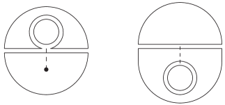
Figure 8: Wilson loop corresponding to the leading part of (C.12).

We can calculate the other terms in the same way and the result is

$$\frac{1}{(\Lambda+1)N}\sum_{l=1}^{\infty}\frac{\lambda^{l}}{(2l)!}\sum_{s}\langle\phi_{s}^{2l}\rangle_{int}$$

$$=\frac{\lambda}{2}\left(\frac{\lambda}{6}-\left(1+\frac{1}{5N^{2}}\right)\frac{\lambda^{2}}{72}+\frac{\lambda^{2}}{36}+\frac{1}{N^{2}}\frac{\lambda^{2}}{180}+\cdots\right)+\frac{\lambda^{2}}{4!}\left(1+\frac{1}{2N^{2}}\right)\frac{2\lambda}{3}+\cdots.$$ (C.13)

Finally, gathering (C.10) and (C.13), we obtain perturbative expansion of the unknot Wilson loop in our matrix model (5.38).

References

- [1] T. Eguchi and H. Kawai, Phys. Rev. Lett. 48, 1063 (1982).
- [2] G. Bhanot, U. M. Heller and H. Neuberger, Phys. Lett. B 113, 47 (1982).
- [3] G. Parisi, Phys. Lett. B 112, 463 (1982).
- [4] D. J. Gross and Y. Kitazawa, Nucl. Phys. B 206, 440 (1982).
- [5] S. R. Das and S. R. Wadia, Phys. Lett. B 117, 228 (1982) [Erratum-ibid. B 121, 456 (1983)].
- [6] A. Gonzalez-Arroyo and M. Okawa, Phys. Rev. D 27, 2397 (1983).
- [7] R. Narayanan and H. Neuberger, Phys. Rev. Lett. 91, 081601 (2003) [arXiv:hep-lat/0303023].
- [8] P. Kovtun, M. Unsal and L. G. Yaffe, JHEP 0706, 019 (2007) [arXiv:hep-th/0702021].
- [9] M. Unsal and L. G. Yaffe, Phys. Rev. D 78, 065035 (2008) [arXiv:0803.0344 [hep-th]].
- [10] B. Bringoltz and S. R. Sharpe, Phys. Rev. D 80, 065031 (2009) [arXiv:0906.3538 [hep-lat]].
- [11] E. Poppitz and M. Unsal, arXiv:0911.0358 [hep-th].
- [12] T. Ishii, G. Ishiki, S. Shimasaki and A. Tsuchiya, Phys. Rev. D 78, 106001 (2008) [arXiv:0807.2352 [hep-th]].
- [13] G. Ishiki, S. Shimasaki, Y. Takayama and A. Tsuchiya, JHEP 0611 (2006) 089 [arXiv:hep-th/0610038].
- [14] T. Ishii, G. Ishiki, S. Shimasaki and A. Tsuchiya, JHEP 0705 (2007) 014 [arXiv:hep-th/0703021].
- [15] T. Ishii, G. Ishiki, S. Shimasaki and A. Tsuchiya, Phys. Rev. D 77 (2008) 126015 [arXiv:0802.2782 [hep-th]].
- [16] M. Hanada, H. Kawai and Y. Kimura, Prog. Theor. Phys. 114, 1295 (2006) [arXiv:hep-th/0508211].
- [17] T. Banks, W. Fischler, S. H. Shenker and L. Susskind, Phys. Rev. D 55 (1997) 5112 [arXiv:hep-th/9610043].
- [18] N. Ishibashi, H. Kawai, Y. Kitazawa and A. Tsuchiya, Nucl. Phys. B 498 (1997) 467 [arXiv:hep-th/9612115].
- [19] R. Dijkgraaf, E. P. Verlinde and H. L. Verlinde, Nucl. Phys. B 500 (1997) 43 [arXiv:hep-th/9703030].
- [20] S. Catterall, arXiv:0909.4532 [hep-lat].
- [21] G. Ishiki, S. W. Kim, J. Nishimura and A. Tsuchiya, Phys. Rev. Lett. 102, 111601 (2009) [arXiv:0810.2884 [hep-th]].
- [22] G. Ishiki, S. W. Kim, J. Nishimura and A. Tsuchiya, JHEP 0909, 029 (2009) [arXiv:0907.1488 [hep-th]].
- [23] Y. Kitazawa and K. Matsumoto, arXiv:0811.0529 [hep-th].
- [24] D. E. Berenstein, J. M. Maldacena and H. S. Nastase, JHEP 0204, 013 (2002) [arXiv:hep-th/0202021].
- [25] M. Hanada, J. Nishimura and S. Takeuchi, Phys. Rev. Lett. 99 (2007) 161602 [arXiv:0706.1647 [hep-lat]].
- [26] K. N. Anagnostopoulos, M. Hanada, J. Nishimura and S. Takeuchi, Phys. Rev. Lett. 100 (2008) 021601 [arXiv:0707.4454 [hep-th]].
- [27] S. Catterall and T. Wiseman, Phys. Rev. D 78, 041502 (2008) [arXiv:0803.4273 [hep-th]].
- [28] J. M. Maldacena, Adv. Theor. Math. Phys. 2 (1998) 231 [arXiv:hep-th/9711200].
- [29] S. S. Gubser, I. R. Klebanov and A. M. Polyakov, Phys. Lett. B 428 (1998) 105 [arXiv:hep-th/9802109].
- [30] E. Witten, Adv. Theor. Math. Phys. 2 (1998) 253 [arXiv:hep-th/9802150].
- [31] E. Witten, Commun. Math. Phys. 121, 351 (1989).
- [32] G. Ishiki, S. Shimasaki and A. Tsuchiya, Phys. Rev. D 80, 086004 (2009) [arXiv:0908.1711 [hep-th]].
- [33] H. Kawai, S. Shimasaki and A. Tsuchiya, arXiv:0912.1456 [hep-th].
- [34] T. Ishii, G. Ishiki, K. Ohta, S. Shimasaki and A. Tsuchiya, Prog. Theor. Phys. 119 (2008) 863 [arXiv:0711.4235 [hep-th]].
- [35] G. Ishiki, K. Ohta, S. Shimasaki and A. Tsuchiya, Phys. Lett. B 672, 289 (2009) [arXiv:0811.3569 [hep-th]].
- [36] M. Marino, Rev. Mod. Phys. 77, 675 (2005) [arXiv:hep-th/0406005].
- [37] M. Marino, arXiv:hep-th/0410165.
- [38] M. Tierz, Mod. Phys. Lett. A 19, 1365 (2004) [arXiv:hep-th/0212128].
- [39] Y. Dolivet and M. Tierz, J. Math. Phys. 48, 023507 (2007) [arXiv:hep-th/0609167].
- [40] M. Blau and G. Thompson, JHEP 0605, 003 (2006) [arXiv:hep-th/0601068].
- [41] Y. Kitazawa, Nucl. Phys. B 642 (2002) 210 [arXiv:hep-th/0207115].
- [42] R. Dijkgraaf and C. Vafa, Nucl. Phys. B 644, 3 (2002) [arXiv:hep-th/0206255]; Nucl. Phys. B 644, 21 (2002) [arXiv:hep-th/0207106]; arXiv:hep-th/0208048.
- [43] A. A. Migdal, Sov. Phys. JETP 42, 413 (1975) [Zh. Eksp. Teor. Fiz. 69, 810 (1975)].
- [44] E. Witten, J. Geom. Phys. 9, 303 (1992) [arXiv:hep-th/9204083].
- [45] J. A. Minahan and A. P. Polychronakos, Nucl. Phys. B 422, 172 (1994) [arXiv:hep-th/9309119].
- [46] D. J. Gross and A. Matytsin, Nucl. Phys. B 429, 50 (1994) [arXiv:hep-th/9404004].
- [47] M. Blau and G. Thompson, arXiv:hep-th/9310144.
- [48] M. Aganagic, A. Klemm, M. Marino and C. Vafa, JHEP 0402, 010 (2004) [arXiv:hep-th/0211098].
- [49] M. Hanada, L. Mannelli and Y. Matsuo, JHEP 0911, 087 (2009) [arXiv:0907.4937 [hep-th]].
- [50] T. T. Wu and C. N. Yang, Nucl. Phys. B 107 (1976) 365.