High Angular Resolution Observations of Four Candidate BLAST High-Mass Starless Cores.

Abstract

We discuss high-angular resolution observations of ammonia toward four candidate high-mass starless cores (HMSCs). The cores were identified by the Balloon-borne Large Aperture Submillimeter Telescope (BLAST) during its 2005 survey of the Vulpecula region where 60 compact sources were detected simultaneously at 250, 350, and 500 µm. Four of these cores, with no IRAS-PSC or MSX counterparts, were mapped with the NRAO Very Large Array (VLA) and observed with the Effelsberg 100 m telescope in the NH₃(1,1) and (2,2) spectral lines. Our observations indicate that the four cores are cold ($T_{\rm k}<16\,$K) and show a filamentary and/or clumpy structure. They also show a significant velocity substructure within $\sim 1\,$km s^-1. The four BLAST cores appear to be colder and more quiescent than other previously observed HMSC candidates, suggesting an earlier stage of evolution.

Table 1: VLA Observing Parameters

BLAST ID	Source Name	RA[J2000]	DEC[J2000]	Synthesized beam	Sensitivity
				arcsec	mJy beam-1
V10	BLAST J194106+235513	19:41:06.5	+23:55:13.5	$3.3\times 2.9$	4.7
V11	BLAST J194136+232325	19:41:36.3	+23:23:24.9	$3.3\times 2.8$	4.3
V27	BLAST J194306+230125	19:43:06.5	+23:01:25.5	$3.4\times 2.7$	4.4
V33	BLAST J194319+232639	19:43:19.0	+23:26:39.6	$3.4\times 3.0$	5.9

Note. — The coordinates represent the BLAST core peak positions and VLA phase tracking center. The synthesized beam and sensitivity refer to the NH₃(1,1) line.

1 INTRODUCTION

The importance of massive ($M\gtrsim 8\,{\rm M}_{\odot}$) stars in shaping the Galactic structure and evolution is well known (Zinnecker & Yorke, 2007). In recent years, a major observational effort has been made to identify the earliest stages of their evolution, which are not very well constrained, yet. Systematic studies by various groups have uncovered several high-mass proto-stellar objects (HMPOs), i.e., dense gravitationally bound cores in a pre-ultracompact (UC) HII region phase with typical temperatures $T\sim 15-90\,$K (Molinari et al., 1996, Molinari et al., 2002, Sridharan et al., 2002, Beuther et al., 2002).

However, these surveys were carried out on IRAS-selected objects and thus there are very few observations of the so-called high-mass starless (or pre-protostellar) core (HMSC) stage, which is supposed to precede the HMPO phase, and their physical and kinematical properties have been barely studied. The survey by Sridharan et al. (2005) was also based on previous observations of IRAS-selected candidate HMPOs at 1.2 mm, thus quite far from the emission peak of the spectral energy distribution (SED) of the coldest ($T\lesssim 15\,$K) cores. The survey of infrared dark clouds (IRDCs) by Pillai et al. (2006) showed that IRDCs are cold ($T<20\,$K) massive ($M>100\,$M_⊙) and have linewidths $\simeq 1-3\,$km s^-1. However, these authors probed regions with typical sizes $\gtrsim 1\,$pc, thus likely to represent pre-protoclusters. Motte et al. (2007) in their unbiased survey of Cygnus X found 17 cores qualifying as good candidates for hosting massive IR-quiet protostars, driving outflows traced by SiO emission, but failed to discover the high-mass analogs of pre-stellar dense cores.

Detailed studies of individual objects (e.g., G28.34+0.06, Wang et al., 2008, Zhang et al., 2009; IRAS 05345+3157, Fontani et al., 2009; Cygnus X, Bontemps et al., 2009) are now contributing to set further constraints on the fragmentation inside massive dense clumps, leading to individual collapsing protostars. These works have tentatively identified cores in very early evolutionary stages, which make them good targets to study the initial fragmentation phases in molecular clumps. In this paper we describe four massive cores that appear to be even colder and more quiescent than similar objects observed in previous works, and may thus further constitute excellent targets for follow-up studies on the initial fragmentation phases.

The Balloon-borne Large Aperture Submillimeter Telescope (BLAST) has recently identified a new and unique sample of massive, cold dust clumps, with characteristics sizes $\lesssim 0.4\,$pc. BLAST is a 2-m stratospheric balloon telescope that observes simultaneously at 250, 350, and 500 µm using bolometric imaging arrays (Pascale et al., 2008). BLAST, until the first Galactic results from Herschel become available, is unique in its ability to detect and characterize cold dust emission from both starless and protostellar sources, constraining the temperatures of objects with $T\lesssim 25$ K using its three-band photometry near the peak of the cold core SED. During the first BLAST science flight (BLAST05), BLAST conducted the first sensitive large-scale Galactic Plane surveys at these wavelengths.

One of the regions observed by BLAST05 covered 4 deg² near the open cluster NGC 6823 in the constellation Vulpecula ($\ell=59^{\circ}$), at a distance of about 2.3 kpc (see discussion in Chapin et al., 2008). In this region, 60 compact sources ($<60^{\prime\prime}$ diameter) were detected simultaneously in all three bands. Their SEDs were constrained through BLAST, IRAS, Spitzer MIPS and MSX photometry, with inferred dust temperatures spanning $\sim 12$–40 K assuming a dust emissivity index $\beta=1.5$, and total masses $\sim 15$–700 $M_{\odot}$ (Chapin et al., 2008). At least 30% of these cores are new, with no IRAS-PSC or MSX associations. Even then, most of those with IRAS identifications have not been studied in detail. The sources detected in the BLAST bands, in particular those without IRAS counterparts, indicate the presence of significant quantities of cool dust. Thus, the BLAST observations resulted in an unique and uniform sample, which may contain a number of bona-fide HMSCs.

Among the 60 compact BLAST sources, we selected the four coldest, massive and IR-quiet cores (see Section 2.1) for observations with the NRAO Very Large Array (VLA) in the NH₃(1,1) and (2,2) spectral lines. The structure of the paper is thus the following: we describe the observations and discuss the main results in Section 2. Our analysis is presented in Section 3 and finally our conclusions are summarized in Section 4.

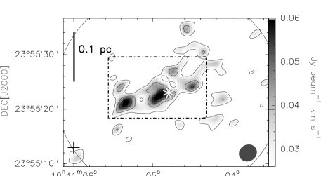
Figure 1: V10. Top. NH₃(1,1) VLA integrated spectrum of V10. Bottom. VLA map of the integrated intensity of NH₃(1,1) over main and satellite components. The first contour level is at +2-$\sigma$ and the interval between adjacent levels is 1-$\sigma$ (RMS $=13\,$mJy beam^-1 km s^-1). The values corresponding to the contour levels are also indicated by the horizontal lines drawn in the grey scale wedge to the right. The ellipse in the bottom right hand corner represents the half power width of the synthesized beam, while the cross indicates the nominal position of the BLAST core (whose uncertainty is $\sim 1\,$arcmin) and the phase tracking center. The pointing position of the 100-m observations is shown by the asterisk and the large solid circle (only partially visible) represents the half power width of the 100-m beam. The dot-dashed box represents the area where the line emission has been integrated to generate the spectrum shown in the top panel. The linear scale in the source is shown by the vertical bar in the left hand side.

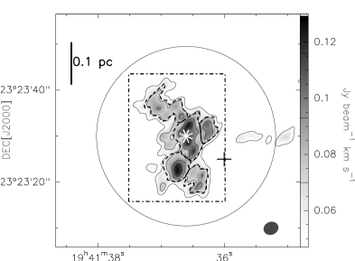
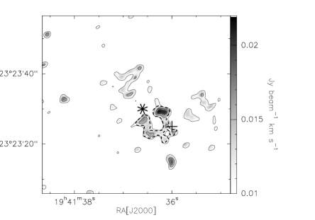
Figure 2: V11. Top. NH₃(1,1) (left) and (2,2) (right) VLA integrated spectra of V11. Bottom. VLA maps of the NH₃(1,1) (left) and (2,2) (right) lines, integrated over the main and satellite (in the case of the (1,1) line) components. The boldface dashed contours in the (1,1) map indicate the specific sub-regions used to calculate the total mass of the source (see Section 3.3). The boldface dashed contour in the (2,2) map indicates the region where emission has been averaged to produce the spectrum shown in Figure 5. Other contours and features are as in Figure 1 (with RMS $=23\,$mJy beam^-1 km s^-1 and $5\,$mJy beam^-1 km s^-1 in the (1,1) and (2,2) maps, respectively).

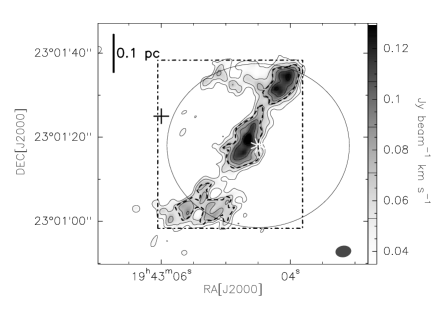
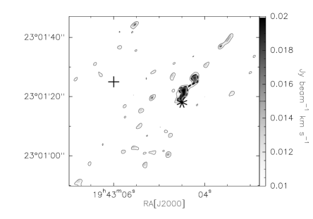
Figure 3: V27. Same as Figure 2 for V27 (with RMS $=18\,$mJy beam^-1 km s^-1 and $5\,$mJy beam^-1 km s^-1 in the (1,1) and (2,2) maps, respectively).

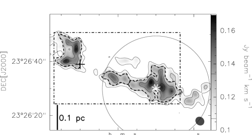
Figure 4: V33. Same as Figure 2 for V33 (with RMS $=27\,$mJy beam^-1 km s^-1 in the (1,1) map), except for the first contour level that here is at 3-$\sigma$. In the bottom panel only the map of the integrated (1,1) emission is shown (see text).

2 OBSERVATIONS AND DATA REDUCTION

2.1 The Sample

Among the starless cores candidates in Vulpecula, i.e. with no IRAS-PSC or MSX counterparts, we selected the four coldest ($T_{\rm dust}<16\,$K) BLAST sources, V10, V11, V27 and V33 (see Table 1), to be observed with the VLA. An analysis of Spitzer IRAC and MIPS images reveals that only source V11 might have an associated protostar, as we discuss later (Section 3.5).

These cores are also massive (with envelope masses $\sim 90$–200 $M_{\odot}$) and both their absolute luminosities ($L_{\rm FIR}\sim 50\,L_{\odot}$) and luminosity-to-mass ratios ($L_{\rm FIR}/M\lesssim 1\,L_{\odot}M_{\odot}^{-1}$, see Figure 18 of Chapin et al., 2008) suggest an early phase of evolution. Qualitatively, this can also be seen by positioning the four sources in the $L-M$ diagram of Molinari et al. (2008) (see their Figure 9), where they would fall in the region representing the early accretion phase. On the same diagram, it can be seen that these BLAST cores are clearly separated from the low-mass regime.

None of the selected sources in Vulpecula is listed in the catalog of Extended Green Objects (EGOs) of Cyganowski et al. (2008), a sample of massive young stellar objects outflow candidates extracted from the GLIMPSE survey (Benjamin et al., 2003). Among the Vulpecula sources that fall in the GLIMPSE survey area (which include V10, V11, V27 and V33) only V09 qualifies as an EGO. This is yet another indication of the early evolutionary phase of the BLAST cores in our sample.

These four Vulpecula cores were observed with the VLA in the NH₃(1,1) and (2,2) spectral lines, which are low-excitation molecular lines, thus appropriate to study the cold cores in the BLAST catalog. In addition, the NH₃ molecule is not expected to be much depleted in pre-stellar cores (e.g., Aikawa et al., 2005), although its exact abundance may depend on the core density (Tafalla et al., 2002, Flower et al., 2006).

2.2 VLA Observations

The VLA ammonia observations were carried out in June 2008, and the array was used in its most compact configuration (D), with baselines from 35 m to 1 km. The NH₃(1,1) and (2,2) inversion lines at 23.694496 and 23.722633 GHz, respectively (Ho & Townes, 1983), were simultaneously observed in the 1IF mode, with a bandwidth of $6.25\,$MHz and 128 channels, corresponding to a velocity coverage of about $80\,$km s^-1 and a velocity resolution of about $0.6\,$km s^-1. The mapped area in each source was $\simeq 2.5\arcmin\times 2.5\arcmin$, centered around the nominal positions of the BLAST cores shown with crosses in Figures 1 to  4 and Figures 6 and 7, and with a synthesized beam FWHM $\simeq 3\,$arcsec (see Table 1). The total time on-source varied from $\simeq 30$ to $\simeq 40\,$min per source and per line. The flux density scale was established by observing 3C48 and the phase calibration was ensured by frequent observations of the point source J19259+21064, that had a measured flux density at the time of the observations of 2.1 Jy. The data were edited and calibrated using the Astronomical Image Processing System (AIPS) following standard procedures. Imaging and deconvolution was performed using the IMAGR task and naturally weighting the visibilities. The resulting observing parameters are listed in Table 1.

Figure 5: NH₃(2,2) VLA spectra toward V11 (top panel) and V27 (bottom panel), obtained by integrating the emission within the boldface dashed contours shown in the (2,2) maps of Figures 2 and 3.

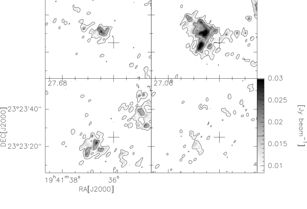
Figure 6: V11. VLA map of NH₃(1,1) main line toward V11, in four adjacent velocity channels (shown in km s^-1 in the top left corner of each panel). The lowest contour level is 2-$\sigma$. The insets show the synthesized beam at half power and the cross indicates the nominal position of the BLAST core and the phase tracking center.

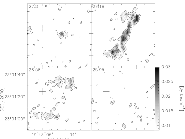
Figure 7: V27. Same as Figure 6 for V27.

Figure 8: V10. NH₃(1,1) spectrum toward V10 taken with the Effelsberg 100-m telescope. The (2,2) emission was not detected.

In order to derive the rotation temperature (Section 3.1) we also need to convert the VLA spectra in units of temperature. The conversion from flux per beam to brightness temperature measured in the synthesized beam, $T_{\rm sb}$, is obtained using the relation (at the frequency of the NH₃(1,1) line):

$$T_{\rm sb}{\rm[K]}=2.18\frac{F_{\nu}{\rm[mJy/beam]}}{\theta_{\rm min}{\rm[\arcsec]}\,\theta_{\rm max}{\rm[\arcsec]}}$$ (1)

where $\theta_{\rm min}$ and $\theta_{\rm max}$ indicate respectively the minor and major axes at half power of the elliptical synthesized beam.

Figure 9: V11. Top. NH₃(1,1) spectrum toward V11 taken with the Effelsberg 100-m telescope. Bottom. NH₃(2,2) spectrum toward V11 smoothed at a velocity resolution of 0.3 km s^-1.

2.3 Effelsberg 100-m Telescope

Single-point spectra of the four BLAST cores were also obtained with the MPIfR 100-m telescope and its 1.3-cm primary focus receiver. The pointing positions used for the 100-m telescope were different from those used with the VLA and are shown as asterisks in Figures 1 to 4. Also shown in these figures is the contour representing the half power width of the 100-m beam. The NH₃(1,1) and (2,2) lines were observed simultaneously within the same band, in position-switched mode (with a beam-throw of $200\,\arcsec$ along the RA direction), with a velocity resolution of $0.077\,$km s^-1 and $\sim 10$ minutes of on-source integration time.

Figure 10: V27. Same as Figure 9 for V27.

The calibration of the 100-m data followed a standard procedure where the arbitrary noise tube units were converted to the antenna temperature scale, and both an atmospheric opacity and elevation corrections have been applied to the antenna gain. The main beam efficiency was $\eta_{\rm mb}=0.52$, the FWHM of the 100-m beam was 39 ″and the resulting noise RMS in the spectra was $\sim 100\,$mK, corresponding to $\sim 60\,$mJy beam^-1 (at the native spectral resolution of $0.077\,$km s^-1).

For comparison with the VLA data (Section 2.5) the 100-m spectra were also converted to Jy using the conversion formula:

$$S_{\rm\lambda}[{\rm Jy}]=2.65\left(\frac{\theta_{\rm mb}[{\rm arcmin}]}{\lambda[{\rm cm}]}\right)^{2}T_{\rm mb}$$ (2)

where $\theta_{\rm mb}$ and $T_{\rm mb}$ are the main-beam FWHM and brightness temperature, respectively.

2.4 VLA Maps and Spectra

As mentioned earlier, the VLA-D has been used to map the NH₃(1,1) and (2,2) inversion transitions. The corresponding maps and integrated spectra (the integration area is represented by the dot-dashed boxes) are shown in Figures 1 to 4. Figures 6 and 7 show channel maps of the NH₃(1,1) main line toward sources V11 and V27. The NH₃(1,1) line has been detected toward all four BLAST cores,whereas the (2,2) transition has been detected in V11, V27 and V33. This is an excellent result, also because the positional errors of the BLAST sources in Vulpecula, which were estimated by Chapin et al. (2008) to be $\sim 7-70\,\arcsec$, could make these detections more difficult.

Figure 11: V33. Same as Figure 9 for V33.

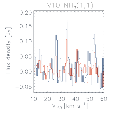
Figure 12: V10. Overlay of the NH₃(1,1) spectra of Effelsberg (blue line) and VLA (red line) in V10.

We note that in V33 a reliable image of the NH₃(2,2) emission could not be produced because of the low signal-to-noise ratio (SNR) and extended emission. However, integration of the emission in a box covering most of the NH₃(1,1) emission yielded a tentative detection of the (2,2) line, as shown in the top-right panel of Figure 4. The hyperfine components have been detected only in the (1,1) line. One can note that, in general, the emission appears to arise from a clumpy and filamentary structure. In V11 and V27 this morphology can be seen even in the weaker (2,2) transition, though at the 2-$\sigma$ level.

Table 2: Velocity, Linewidth and Total Optical Depth from Method NH₃(1,1).

	VLAa					100-m
Source	$T_{\rm ex}$	$V_{\rm lsr}$	$\Delta V$	$\tau$		$T_{\rm ex}$	$V_{\rm lsr}$	$\Delta V$	$\tau$
	K	km s-1	km s-1			K	km s-1	km s-1
V10	$4.2\pm 1.2$	$33.52\pm 0.07$	$<1.0$	$1.8\pm 1.0$		$3.23\pm 0.25$	$33.69\pm 0.02$	$0.41\pm 0.05$	$3.0\pm 0.9$
V11	$5.0\pm 1.1$	$28.24\pm 0.04$	$<1.0$	$2.0\pm 0.7$		$3.97\pm 0.27$	$28.12\pm 0.01$	$0.83\pm 0.03$	$2.1\pm 0.3$
V27	$5.5\pm 2.2$	$27.00\pm 0.03$	$<1.0$	$0.7\pm 0.5$		$4.63\pm 0.40$	$26.98\pm 0.01$	$0.70\pm 0.03$	$1.6\pm 0.2$
V33	$4.3\pm 0.4$	$22.21\pm 0.03$	$<1.0$	$2.5\pm 0.4$		$4.97\pm 0.25$	$22.26\pm 0.01$	$0.66\pm 0.02$	$2.2\pm 0.2$

The velocity scale shown in the spectra of Figures 1 to 4 (and also in all subsequent spectra) is referred to the NH₃(1,1) and (2,2) main lines. We note the excellent agreement with the velocities estimated by Chapin et al. (2008) using ¹³CO$(1-0)$. All spectral lines are clearly very narrow and the VLA observations do not resolve the lines (see later Section 3.1 and Tables 2 and 3). In the case of the (1,1) maps of sources V11 and V27 one can note in Figures 6 and 7 the sharp change in the brightness spatial distribution in adjacent velocity channels. This indicates a significant velocity substructure within $\sim 1\,$km s^-1. In V11 and V27 these features are unlikely to be a consequence of missing flux, since with the VLA-D we recover most of the flux measured by the 100-m telescope (see Section 2.5).

Although the morphological difference between these sources could be caused by both intrinsic (e.g., geometrical effects and/or different evolutionary phases) and observational effects, all these cores present very similar features. In fact, they all show an internal structure, with both smaller cores, or fragments, and an inter-core emission, which also appears to be “filamentary”. The fragments inside the cores have sizes $\lesssim 0.05\,$pc and we are unable to resolve structures smaller than $\simeq 0.034\,$pc (7100 AU).

2.5 Effelsberg Spectra

The Effelsberg telescope was used to observe the four BLAST sources toward their central positions at higher spectral resolution. The resulting spectra are shown in Figures 8 to 11, where we note that the hyperfine components of both the inner and outer satellites are partly resolved, an indication of the narrow linewidths in this source.

For comparison with the VLA, the spectra obtained with the 100-m telescope were resampled at the same spectral resolution as the VLA, and the results are shown in Figures 12 to 15. The flux measured by the VLA is almost always (exceptions are the NH₃(2,2) spectra toward V11 and V33) lower than that observed with the 100-m telescope, probably as a result of both low SNR in the VLA spectra and extended emission that is filtered out by the interferometer. If we compare the main-line emission, the amount of the single-dish flux lost by the VLA varies from $\simeq 20-30\,$% in V27 and V11 to $\simeq 50\,$% in V10 and V33. In V11 and V33 the VLA recovers most of the NH₃(2,2) single-dish flux.

3 ANALYSIS

3.1 Derivation of Physical Parameters with METHOD NH₃(1,1)

The NH₃(1,1) and (2,2) inversion lines show an electric quadrupole and magnetic hyperfine structure (see Ho & Townes, 1983 for a review). The (1,1) spectra were fitted using a non-linear least-square method (METHOD NH₃(1,1) of the CLASS program) which takes into account the 18 hyperfine components. This method can determine the optical depths and linewidths assuming that all components have equal excitation temperatures, that the line separation is fixed at the laboratory value and that the linewidths are identical.

The NH₃(2,2) lines are weaker and the sensitivity of these observations is less than the sensitivity of the NH₃(1,1) data. Thus, the quadrupole hyperfine structure of the NH₃(2,2) transition is not visible when the emission is averaged over the same large area as the (1,1) line, shown by the dot-dashed boxes in Figures 1 to 4. The hyperfine structure of the (2,2) line becomes visible in sources V11 and V27 (see Figure 5) only when the emission is averaged on smaller sub-regions, such as the ones shown by the boldface dashed contours in Figures 2 and 3. Therefore, for the purpose of using METHOD NH₃(1,1) of the CLASS program we always fitted the (2,2) profiles (obtained by integrating the VLA maps in the same region as the (1,1) transition) by simple Gaussians. Due to the hidden magnetic hyperfine structure, this tends to overestimate the intrinsic linewidths (Bachiller et al., 1987).

The results of the NH₃(1,1) fitting are listed in Table 2. The 100-m spectra have the advantage of a better SNR and spectral resolution and therefore the derived parameters are more accurate, though they do not necessarily describe the same volume of gas. The effect of the better spectral resolution is clearly visible in the resulting linewidths (see Table 2). As mentioned earlier the VLA does not resolve the lines and thus the VLA linewidths should be interpreted only as upper limits. On the other hand the 100-m results show that the linewidths are indeed different and very narrow. A temperature of $T_{\rm k}=14\,$K corresponds to a NH₃ thermal linewidth of $\Delta V_{\rm th}=0.19\,$km s^-1 ($\Delta V_{\rm th}=\sqrt{8\,\ln 2\,kT_{\rm k}/(17\,m_{\rm H})}$, where $k$ is the Boltzmann constant and $m_{\rm H}$ is the atomic hydrogen mass). Therefore, non-thermal motions definitely give an important contribution in these sources. The overall linewidths, however, are smaller (or much smaller in the case of V10) than those previously observed toward (warmer) HMPOs by, e.g., Molinari et al. (1996), who found median linewidths $\simeq 1.7-1.8$ km s^-1, and also by Motte et al. (2007) who found linewidths $\gtrsim 2.0$ km s^-1.

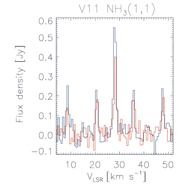
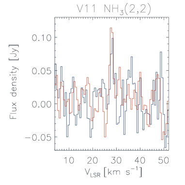
Figure 13: V11. Top. Overlay of the NH₃(1,1) spectra of Effelsberg (blue line) and VLA (red line) in V11. Bottom. Same as above for NH₃(2,2).

Table 3: Results of Gaussian Fits to the NH₃(2,2) Lines.

	VLA				100-m
Source	$T_{\rm sb}$	$V_{\rm lsr}$	$\Delta V$		$T_{\rm mb}$	$V_{\rm lsr}$	$\Delta V$
	K	km s-1	km s-1		K	km s-1	km s-1
V11	$0.46\pm 0.09$	$27.91\pm 0.13$	$1.4\pm 0.3$		$0.16\pm 0.06$	$28.23\pm 0.19$	$1.44\pm 0.56$
V27	$0.24\pm 0.06$	$27.13\pm 0.15$	$1.3\pm 0.3$		$0.33\pm 0.06$	$26.96\pm 0.08$	$1.23\pm 0.18$
V33	$0.62\pm 0.14$	$22.27\pm 0.13$	$<1.0$		$0.52\pm 0.09$	$22.36\pm 0.04$	$0.72\pm 0.08$

Note. — The VLA fits have been performed on the integrated spectra in the area shown by the dot-dashed boxes in Figures 2 to 4.

Source V11 has the largest linewidth, as measured by both (1,1) and (2,2) lines. We also note that V11 is the only source where the velocity structure shown in Figure 6 is suggesting the presence of either two cores at separate velocities or a velocity gradient, positive S to N, of $\simeq 11\,$km s^-1 pc^-1. Neither of these can be ruled out on the basis of the present data. Incidentally, V11 is also the only source with a clear positional association with a likely protostar (see Section 3.5).

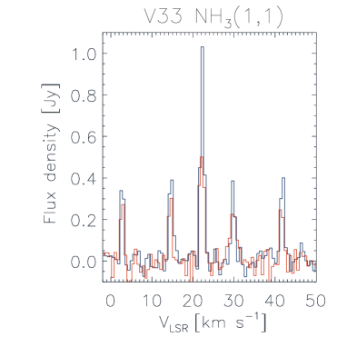
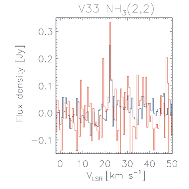
Figure 15: V33. Same as Figure 13 for V33.

The results of the Gaussian fits to the NH₃(2,2) profiles are listed in Table 3. Because the Gaussian fit does not take into account the hyperfine structure of the line, we cannot compare directly the linewidths in Tables 2 and 3. We also note the same basic behaviour among those sources with a (2,2) detection: source V33 has in fact the smallest linewidth as measured by both (1,1) and (2,2) lines. However, because in the VLA spectrum the (2,2) line is barely two channels wide (see Figure 15) in Table 3 we only list an upper limit.

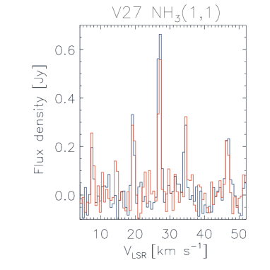
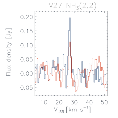
Figure 14: V27. Same as Figure 13 for V27.

Table 4: Temperature and Column Density

	VLAa				100-m
Source	$T_{12}$	$T_{\rm k}$	$N({\rm NH_{3}})$		$T_{12}$	$T_{\rm k}$	$N({\rm NH_{3}})$
	K	K	$\times 10^{14}$ cm-2		K	K	$\times 10^{14}$ cm-2
V11	$10.5\pm 0.5$	$11.1\pm 0.6$	$21.5\pm 4.7$		$11.9\pm 1.1$	$12.8\pm 1.3$	$6.6\pm 1.0$
V27	$8.7\pm 0.5$	$9.0\pm 0.6$	$34.1\pm 8.4$		$14.3\pm 0.6$	$16.0\pm 1.0$	$3.9\pm 0.4$
V33	$9.2\pm 0.2$	$9.5\pm 0.2$	$37.8\pm 6.7$		$12.2\pm 0.3$	$13.1\pm 0.5$	$6.5\pm 0.4$

3.2 Temperature

In V11, V27, and V33, where the (2,2) line was detected, we were also able to determine the rotation temperature, $T_{\rm 12}$ (and thus the kinetic temperature $T_{\rm k}$), and the column density using the method of Ungerechts et al. (1986) and Bachiller et al. (1987). In this method the required data were: (i) the product $\tau(T_{\rm ex}-T_{\rm bg})$ for the (1,1) line, where $T_{\rm ex}$ and $T_{\rm bg}=2.725\,$K are the excitation and background temperatures, respectively, and $\tau$ is the optical depth; (ii) the linewidth $\Delta V(1,1)$; and (iii) the (2,2) integrated intensity. Once $T_{\rm 12}$ has been estimated, the kinetic temperature can be determined using the analytical expression of Tafalla et al. (2004):

$$T_{\rm k}=\frac{T_{\rm 12}}{1-\frac{T_{\rm 12}}{42}\ln[1+1.1\exp(-\frac{16}{T_{\rm 12}})]}$$ (3)

which is an empirical expression that fits the $T_{\rm 12}-T_{\rm k}$ relation obtained using a radiative transfer model.

The results are shown in Table 4. The VLA physical parameters represent average values, estimated by first integrating the NH₃(1,1) in the smaller sub-regions enclosed by the boldface dashed contours shown in Figures 2 to 4 (see also Sect. 3.3); then, the parameters obtained in each of these sub-regions have been averaged together and the results listed in Table 4. Because of the coarse spectral resolution of the VLA spectra, when evaluating the physical parameters from the VLA data we have replaced the original linewidths with the 100m linewidths. Although the 100m linewidths represent themselves averages over a larger source area compared to the smaller sub-regions shown in Figures 2 to 4, they give a better estimate of the $\Delta V(1,1)$ values as compared to the upper limits given by the VLA linewidths. In addition, because of the weakness of the (2,2) transition, we could not obtain separate (2,2) integrated spectra for the sub-regions. As a consequence, we have always used the NH₃(2,2) spectrum obtained by integrating over the entire source, as shown in Figures 2 to 4.

The small linewidths listed in Table 2 and the low kinetic temperatures of Table 4 again suggest small internal motions and therefore very quiescent conditions. The four BLAST cores appear to be even colder and more quiescent than the HMSC candidates observed by Sridharan et al. (2005), who found in their sample of candidate HMSCs a median linewidth of 1.5 km s^-1, comparable with that of Molinari et al. (1996), and a median rotation temperature of 16.9 K. The average temperature of our cores is also somewhat lower than the mean kinetic temperature of 15 K found in IRDCs by Pillai et al. (2006).

Table 5: Size, Mass and Density

Source	Diametera			$M_{\rm BLAST}^{\rm b}$	$M_{\rm vir}$	$M_{\rm tot}^{\rm c}$			$\langle n_{\rm H_{2}}\rangle^{\rm c}$
	arcsec	pc		$M_{\odot}$	$M_{\odot}$	$M_{\odot}$	$M_{\odot}$		$\times 10^{5}\,$cm-3	$\times 10^{5}\,$cm-3
V10	7.6	0.08		89	1.5	-	-		-	-
V11	12.6	0.14		213	10.2	5.0	72.0		2.2	31.0
V27	11.6	0.13		105	6.7	9.7	138.5		2.3	33.4
V33	18.8	0.21		107	9.6	21.0	300.7		2.1	30.0

Note. — $M_{\rm tot}$ represents the total mass of the source as estimated by summing the masses ($M_{\rm cd}$) of the sub-regions enclosed by dashed contours shown in Figures 2 to 4. $\langle n_{\rm H_{2}}\rangle$ represents the average density among the sub-regions in which each source has been divided.

3.3 Column Density and Mass

The three fitting parameters described in Section 3.2 may also be used to determine the column densities, $N(1,1)$ and $N(2,2)$, of the (1,1) and (2,2) lines. Then, the total NH₃ column density, $N_{\rm NH_{3}}$, is obtained from $T_{\rm 12}$ using the method of Ungerechts et al. (1986). The total mass in the VLA maps has been estimated by dividing each source into smaller sub-regions (shown by the boldface dashed contours in Figures 2 to 4) and determining $N_{\rm NH_{3}}$ in each of them. The approximate size of each region represents a trade-off between the need to achieve a good SNR in the integrated spectra of each region, and the need to avoid integrating over too large an area with no NH₃ emission. For the VLA data, the values of temperatures and column densities averaged in these sub-regions in sources V11, V27 and V33 are listed in Table 4

As an example of the NH₃(1,1) spectra and line fits obtained with this procedure we show in Figure 16 the spectra obtained toward V27 by integrating the emission in the three smaller areas, enclosed within dashed contours, shown in Figure 2. As mentioned already in Section 3.2, for each sub-region we have used the same NH₃(2,2) spectrum obtained by integrating over the entire source. In addition, the NH₃(1,1) linewidths have been kept fixed, and equal to the 100m values, during the fits to the VLA spectra obtained using METHOD NH₃(1,1) of CLASS, such as the ones shown Figure 16. The total mass of each source can then be computed by adding the masses of the individual sub-regions, estimated as:

$$M_{\rm cd}=1.38\,\frac{\pi}{4}D^{2}\,N_{\rm H_{2}}\,m_{\rm H_{2}}$$ (4)

where $D$ is the sub-region diameter, $m_{\rm H_{2}}$ is the mass of the H₂ molecule, $N_{\rm H_{2}}$ is the sub-region averaged column density and 1.38 is the correction factor for the abundance of helium and heavier elements in the interstellar medium. The source diameter is actually an equivalent diameter calculated as $\sqrt{\Omega_{\rm s}/1.133}$, where $\Omega_{\rm s}$ represents the solid angle covered by the individual sub-regions shown in Figures 2 to 4. We have evaluated $M_{\rm cd}$ for two possible values of the ammonia abundance, corresponding to the minimum and maximum values found in Table 3 of Pillai et al. (2006), $X[{\rm NH_{3}}]=7\times 10^{-9}$ and $X[{\rm NH_{3}}]=10^{-7}$. The corresponding values of $M_{\rm cd}$ are listed separately in Table 5 (columns 6 and 7). The particle density has then been calculated as:

$$n_{\rm H_{2}}=\frac{3M_{\rm cd}}{4\pi(D/2)^{3}\mu\,m_{\rm H}}$$ (5)

where $\mu=2.33$ is the mean molecular weight per particle and $m_{\rm H}$ is the mass of the hydrogen atom. The two values of $n_{\rm H_{2}}$ corresponding to the choice of $X[{\rm NH_{3}}]$ are also listed separately in Table 5 (columns 8 and 9).

From the linewidths of the observed transitions and the estimated source angular diameters we can also derive the mass required for virial equilibrium. Assuming the source to be spherical and homogeneous (an assumption which is not, however, well justified in all of our sources), and neglecting contributions from magnetic field and surface pressure, the virial mass is given by (MacLaren et al., 1988):

$$M_{\rm vir}{\rm[M_{\odot}]}=0.509\,d{\rm[kpc]}\,\theta_{\rm s}{\rm[arcsec]}\,(\Delta V{\rm[km/s]})^{2}$$ (6)

where $d=2.3\,$kpc (Chapin et al., 2008) is the distance to the four BLAST sources. The estimated virial masses (column 5 in Table 5) show that the cores are more likely to be gravitionally unstable, even when the largest value of $X[{\rm NH_{3}}]=10^{-7}$ is used, are V33 and, to a lesser extent, V27. Source V11 seems to be closer to virial equilibrium, compared to V27 and V33, which would appear to be consistent with V11 being a proto-stellar core (see Section 3.5). For comparison, the virial masses listed in Table 5 are quite smaller compared to the values estimated by Fontani et al. (2004) for comparable sizes. However, these authors did not use their NH₃ map and spectra to determine the virial mass, and they measured much larger linewidths in other molecular tracers. Therefore, the virial masses of Fontani et al. (2004) are likely to reflect the much larger degree of turbulence in HMPOs.

Furthermore, apart from the various approximations involved in the calculation of $M_{\rm vir}$, its comparison with the masses obtained by the fit to the spectral energy distribution (with assumed values of the dust mass absorption coefficient at 250 µm, $k_{\rm 250}=10\,$cm²g^-1, and a dust emissivity index, $\beta=1.5$, Chapin et al., 2008) is further complicated by the fact that the BLAST05 observations were sensitive to cold dust on a much larger scale ($\gtrsim 1\,$arcmin).

The comparison between $M_{\rm tot}$ and $M_{\rm vir}$ in Table 5 is complicated by the many uncertainty factors. In addition, for a power-law density distribution of the type $n_{\rm H_{2}}(r)\propto r^{-m}$, the virial mass obtained from Eq. (6) must be multiplied by a factor $\frac{3}{5}\,\frac{5-2m}{3-m}$ (see MacLaren et al., 1988). For example, Fontani et al. (2004) found that $m=2.3$ in the HMPO IRAS 23385+6053 and thus their virial masses had to be multiplied by a factor $\simeq 0.35$.

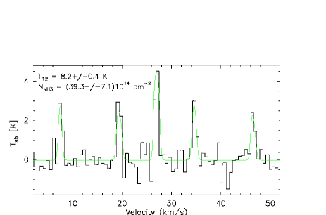
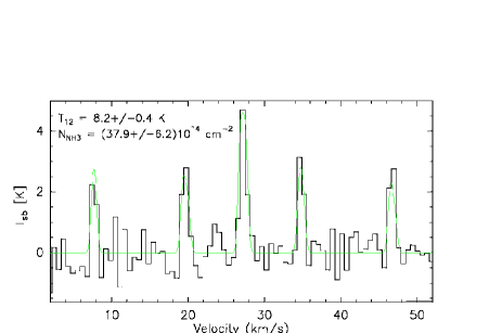
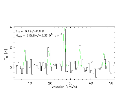
Figure 16: VLA spectra obtained towards V27 by selecting the three smaller sub-regions enclosed by the boldface dashed contours shown in Figure 3. The solid line represents the fit obtained with METHOD NH₃(1,1) of the CLASS program, by setting the VLA linewidths to the 100m values (see text). Also shown are the values of the rotation temperature (Section 3.2) and NH₃ column density as obtained in each separate sub-region (see Section 3.3 and Table 4, where the parameters listed are weighted averages).

3.4 Comparison with Low-Mass Pre-Stellar Cores

To analyze the origin of the V10, V11, V27 and V33 cores, we can compare the properties of these cores with the well-studied low-mass pre-stellar core L1544 in the Taurus molecular cloud (at a distance of 140 pc) that appears to be gravitationally unstable (for a review see Doty et al., 2005 and references therein). The L1544 core has a continuum source with a flux density of 17.4 Jy at 450 µm (Shirley et al., 2000), corresponding to a gas+dust mass of 3.2 M_⊙, and a density of $1.5\times 10^{6}\,$cm^-3 (Ward-Thompson et al., 1999). The N₂H⁺ linewidth toward L1544 is 0.3 km s^-1, and observations toward several low-mass starless cores in NH₃ and N₂H⁺ show similar linewidths for both molecules (Tafalla et al., 2004).

In order to compare the physical properties of L1544 with those of the BLAST cores listed in Table 5, we note that the peak NH₃ abundance determined by Tafalla et al. (2002) toward L1544 was $4.0\times 10^{-9}$. Therefore, if we consider the physical parameters in Table 5 corresponding to the lower value of the NH₃ abundance ($7.0\times 10^{-9}$, close enough to that estimated in L1544), we see that the number density in the BLAST cores is quite similar to that of L1544, while their mass is a factor of $\sim 20-100$ higher, and is quite higher even when one considers the masses of the smaller sub-regions within each source, as described in Section 3.3.

As far as the velocity dispersion is concerned, the BLAST cores have NH₃ linewidths more than double that of L1544, with the exception of V10 which has a linewidth (0.41 km s^-1, see Table 2) only slightly higher than that of L1544. This would be consistent with the BLAST cores being more turbulent and could also possibly hide other systematic internal motions (see the case of V11, Section 3.1).

What would a core like L1544 appear in the BLAST05 map of Vulpecula? Scaling the 450 µm L1544 emission to 500 µm at a distance of 2.3 kpc, we would expect an integrated flux density of about 40 mJy and thus it would go undetected in the BLAST05 map of Vulpecula (Chapin et al., 2008). This is consistent with the four BLAST sources being separated, if they were plotted on the $L-M$ diagram of Molinari et al. (2008), from the low-mass regime, as mentioned in Section 2.1.

Table 5 shows that only in the case of V11 the total mass inferred from the BLAST observations is significantly larger than the mass estimate based on NH₃ emission, given the NH₃ abundance range that we have selected. In V27 and V33, the mass range obtained from our observations is consistent with the BLAST mass estimate. It is possible that in the case of V11 the ammonia emission results from only a small fraction of molecular material that is concentrated in a denser and more compact structure. A similar scenario, for example, has been found by Shepherd et al. (2004) toward the core G192 S3, and it could also be the case in V27 and V33 if the NH₃ abundance were near the upper limit of the range listed in Table 5. In this case, an interesting question would be whether the mass determined from the VLA NH₃ observations represents the total reservoir from which any star formation will eventually take place in these cores or, rather, further mass will be accreted from the larger mass reservoir detected by BLAST. In the first scenario, it is unlikely that these cores will produce massive stars, unless the total gas and dust mass is much higher, as it would result if $X[{\rm NH_{3}}]<<10^{-7}$.

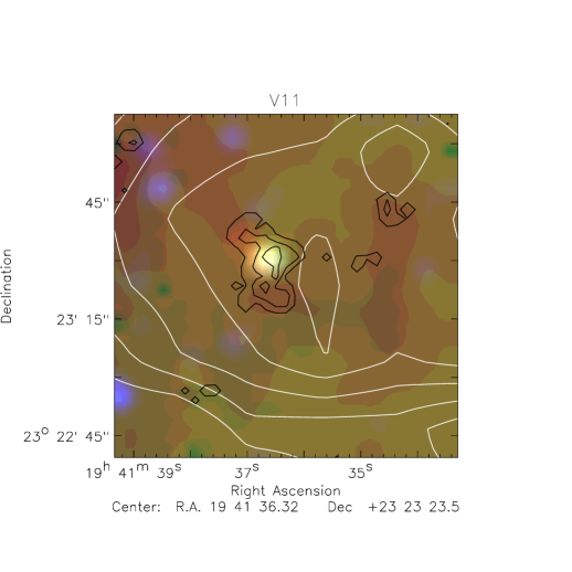
Figure 17: Three-color Spitzer image 3.6 µm (blue), 8 µm (green), and 24 µm (red) of V11 (at the angular resolution of the MIPS 24 µm map). The overlaid white, solid contours represent the BLAST 350 µm emission (from $4.3\times 10^{7}$ to $1.2\times 10^{8}$ by $1.6\times 10^{7}$ Jy srad^-1). The black, solid contours represent the integrated NH₃(1,1) VLA emission (from 0.039 to 0.112 by 0.036 Jy beam^-1 km s^-1).

Likewise, one might ask whether the lower-mass fragments in these regions could at a later stage merge to form a more massive pre-stellar core that could then evolve toward a high-mass star. Clearly, we cannot currently determine the relative motions of the individual fragments in the observed cores. However, we can use the NH₃ linewidths as a rough estimate of the average turbulent motion, though they do not necessarily represent the relative velocities of coherent sub-structures within the cores. If we take $\sim 0.1$ pc and $0.8\sqrt{3}$ km s^-1 as the typical fragment (de-projected) separation and 3D velocity dispersion, respectively, we obtain a time-scale $\sim 8\times 10^{4}$ yr. Although this time-scale is comparable to the accretion time-scales estimated by Bonnell & Bate (2006) for the formation of high-mass stars in the competitive accretion scenario, the most significant individual fragments inside the cores appear to be more massive than the thermal Jeans mass ($\sim 1\,M_{\odot}$), which is inconsistent with the model of Bonnell & Bate (2006) for competitive accretion. Alternatively, it is quite possible that we are observing these cores at a phase when merging of low-mass fragments has already occurred, and that the less significant fragments in Figures 1 to 4, with masses $\gtrsim 1\,M_{\odot}$, are actually the remnants of this accreting phase.

3.5 Evolutionary Phase of the Cores

As we have seen in Section 3.2 and Section 3.3, our cores have similar temperatures but are more compact, and possibly less massive (depending on the NH₃ abundance), than IRDCs, which have a typical size $\gtrsim 1\,$pc. This suggests that they may be similar to the unresolved cores found toward IRDCs, but in an earlier stage of evolution compared to the sources observed by Molinari et al. (1996) and Sridharan et al. (2005).

This conclusion is supported by the lack of an IRAS and MSX counterpart to these sources, as mentioned in Section 2.1. However, we have also inspected the IRAC and MIPS images and found that only in the case of V11 an IRAC/MIPS point source is found to be positionally coincident with the NH₃(1,1) integrated emission. As shown in Figure 17 this source has the colors expected for an embedded protostar. Aperture photometry confirms that the SED of this infrared source is rising between 3.6 and 24 µm. However, we find no point source in the 70 µm MIPS image. No other infrared source with similar colors is found within $\simeq 1\,$arcmin from the peak of either the NH₃(1,1) or the BLAST emission. Together with the larger linewidth and a more systematic velocity shift across the source structure, as discussed in Section 3.1, these properties suggest that V11 is probably the most evolved of all four observed cores, and is likely to harbour a protostar.

In addition, we have also searched for possible radio continuum emission toward the four Vulpecula sources. In order to do this we have analyzed both the continuum images constructed from the line-free channels of our VLA observations, and the available maps from the CORNISH survey of the Galactic Plane (Purcell et al., 2008). We do not detect any continuum emission at the level of $\simeq 0.4\,$mJy beam^-1, in our line-free channels maps, which is about the same as the noise level achieved at 5 GHz in the CORNISH maps. Thus, both the upper limit to the continuum emission (see Purcell et al., 2008) and the luminosity estimated from SED fits ($L\sim 50\,L_{\odot}$, Chapin et al., 2008) imply an ionizing source much less than a B3 zero-age main-sequence star. The low-luminosity in the radio continuum could be because the central object has not yet developed an UC HII region, or because of opacity if the surroundings of the protostar (if any) are very dense.

4 CONCLUSIONS

We have observed four candidate high-mass starless cores selected from the BLAST05 survey of the Vulpecula region. Our VLA-D observations in the NH₃(1,1) and (2,2) lines suggest that these cores are in very early stages of evolution, prior to the formation of a (proto)star or proto-cluster. In only one of these cores, V11, the VLA peak emission of NH₃(1,1) is associated with an infrared source having the colors expected for an embedded protostar. The four cores are cold ($T_{\rm k}<16\,$K), relatively quiescent ($\Delta V\lesssim 0.8\,$km s^-1) but with a higher velocity dispersion compared to e.g., L1544, and show a filamentary and clumpy structure. Our VLA-D data have limited spectral resolution, but we can clearly observe a significant velocity substructure within $\sim 1\,$km s^-1.

Based on the comparison with a typical low-mass pre-stellar core, we find that these BLAST cores are more massive and more luminous. V11 is likely to have already formed an intermediate-mass (proto)star and given the mass range obtained for V27 and V33 they too could form intermediate- or even high-mass stars. However, a confirmation of this conclusion will require a more accurate determination of the NH₃ abundance in these cores.

References

- Aikawa et al. (2005) Aikawa, Y., Herbst, E., Roberts, H., & Caselli, P. 2005, ApJ, 620, 330
- Bachiller et al. (1987) Bachiller, R., Guilloteau, S., & Kahane, C. 1987, A&A, 173, 324
- Benjamin et al. (2003) Benjamin, R. A., Churchwell, E., Babler, B. L., Bania, T. M., Clemens, D. P., Cohen, M., Dickey, J. M., Indebetouw, R., Jackson, J. M., Kobulnicky, H. A., Lazarian, A., Marston, A. P., Mathis, J. S., Meade, M. R., Seager, S., Stolovy, S. R., Watson, C., Whitney, B. A., Wolff, M. J., & Wolfire, M. G. 2003, PASP, 115, 953
- Beuther et al. (2002) Beuther, H., Schilke, P., Menten, K. M., Motte, F., Sridharan, T. K., & Wyrowski, F. 2002, ApJ, 566, 945
- Bonnell & Bate (2006) Bonnell, I. A. & Bate, M. R. 2006, MNRAS, 370, 488
- Bontemps et al. (2009) Bontemps, S., Motte, F., Csengeri, T., & Schneider, N. 2009, ArXiv e-prints
- Chapin et al. (2008) Chapin, E. et al. 2008, ApJ, 681, 428
- Cyganowski et al. (2008) Cyganowski, C. J., Whitney, B. A., Holden, E., Braden, E., Brogan, C. L., Churchwell, E., Indebetouw, R., Watson, D. F., Babler, B. L., Benjamin, R., Gomez, M., Meade, M. R., Povich, M. S., Robitaille, T. P., & Watson, C. 2008, AJ, 136, 2391
- Doty et al. (2005) Doty, S. D., Everett, S. E., Shirley, Y. L., Evans, N. J., & Palotti, M. L. 2005, MNRAS, 359, 228
- Flower et al. (2006) Flower, D. R., Pineau Des Forêts, G., & Walmsley, C. M. 2006, A&A, 456, 215
- Fontani et al. (2004) Fontani, F., Cesaroni, R., Testi, L., Walmsley, C. M., Molinari, S., Neri, R., Shepherd, D., Brand, J., Palla, F., & Zhang, Q. 2004, A&A, 414, 299
- Fontani et al. (2009) Fontani, F., Zhang, Q., Caselli, P., & Bourke, T. L. 2009, VizieR Online Data Catalog, 349, 90233
- Ho & Townes (1983) Ho, P. T. P. & Townes, C. H. 1983, ARA&A, 21, 239
- MacLaren et al. (1988) MacLaren, I., Richardson, K. M., & Wolfendale, A. W. 1988, ApJ, 333, 821
- Molinari et al. (1996) Molinari, S., Brand, J., Cesaroni, R., & Palla, F. 1996, A&A, 308, 573
- Molinari et al. (2008) Molinari, S., Pezzuto, S., Cesaroni, R., Brand, J., Faustini, F., & Testi, L. 2008, A&A, 481, 345
- Molinari et al. (2002) Molinari, S., Testi, L., Rodríguez, L. F., & Zhang, Q. 2002, ApJ, 570, 758
- Motte et al. (2007) Motte, F., Bontemps, S., Schilke, P., Schneider, N., Menten, K. M., & Broguiére, D. 2007, A&A, 476, 1243
- Pascale et al. (2008) Pascale, E. et al. 2008, ApJ, 681, 400
- Pillai et al. (2006) Pillai, T., Wyrowski, F., Carey, S. J., & Menten, K. M. 2006, A&A, 450, 569
- Purcell et al. (2008) Purcell, C. R., Hoare, M. G., & Diamond, P. 2008, in Astronomical Society of the Pacific Conference Series, Vol. 387, Massive Star Formation: Observations Confront Theory, ed. H. Beuther, H. Linz, & T. Henning, 389
- Shepherd et al. (2004) Shepherd, D. S., Borders, T., Claussen, M., Shirley, Y., & Kurtz, S. 2004, ApJ, 614, 211
- Shirley et al. (2000) Shirley, Y. L., Evans, II, N. J., Rawlings, J. M. C., & Gregersen, E. M. 2000, ApJS, 131, 249
- Sridharan et al. (2005) Sridharan, T. K., Beuther, H., Saito, M., Wyrowski, F., & Schilke, P. 2005, ApJ, 634, L57
- Sridharan et al. (2002) Sridharan, T. K., Beuther, H., Schilke, P., Menten, K. M., & Wyrowski, F. 2002, ApJ, 566, 931
- Tafalla et al. (2004) Tafalla, M., Myers, P. C., Caselli, P., & Walmsley, C. M. 2004, A&A, 416, 191
- Tafalla et al. (2002) Tafalla, M., Myers, P. C., Caselli, P., Walmsley, C. M., & Comito, C. 2002, ApJ, 569, 815
- Ungerechts et al. (1986) Ungerechts, H., Winnewisser, G., & Walmsley, C. M. 1986, A&A, 157, 207
- Wang et al. (2008) Wang, Y., Zhang, Q., Pillai, T., Wyrowski, F., & Wu, Y. 2008, ApJ, 672, L33
- Ward-Thompson et al. (1999) Ward-Thompson, D., Motte, F., & André, P. 1999, MNRAS, 305, 143
- Zhang et al. (2009) Zhang, Q., Wang, Y., Pillai, T., & Rathborne, J. 2009, ApJ, 696, 268
- Zinnecker & Yorke (2007) Zinnecker, H. & Yorke, H. W. 2007, ARA&A, 45, 481