A spatial model of autocatalytic reactions

Abstract

Biological cells with all of their surface structure and complex interior stripped away are essentially vesicles — membranes composed of lipid bilayers which form closed sacs. Vesicles are thought to be relevant as models of primitive protocells, and they could have provided the ideal environment for pre-biotic reactions to occur. In this paper, we investigate the stochastic dynamics of a set of autocatalytic reactions, within a spatially bounded domain, so as to mimic a primordial cell. The discreteness of the constituents of the autocatalytic reactions gives rise to large sustained oscillations, even when the number of constituents is quite large. These oscillations are spatio-temporal in nature, unlike those found in previous studies, which consisted only of temporal oscillations. We speculate that these oscillations may have a role in seeding membrane instabilities which lead to vesicle division. In this way synchronization could be achieved between protocell growth and the reproduction rate of the constituents (the protogenetic material) in simple protocells.

I Introduction

The cell is a structural and functional unit, the building block of any living system. Cells consist of a membrane, made of a lipid bilayer, which encloses and protects the contents of the cell, including genetic material. The membrane is semi-permeable: nutrients can diffuse in and serve as energy to support the functioning of the machinery alb02 . Cells undergo replication (cell division): this is a process by which a cell, hereafter called the parent cell, divides into two or more cells, called the daughters. The daughter cell contains in principle an exact replica of the parent’s inner constituents, this property being ultimately a prerequisite for stable living organisms to exist. Such a process clearly relies on the synchronization between the duplication rate of the constituents and the growth of the container. In modern cells this condition is of paramount importance and is efficiently realized via dedicated control mechanisms, expressed as pathways of nested molecular checkpoints alb02 . This complex and delicate machinery has evolved; presumably the first minimalistic cells (so-called protocells dea86 -ras08 ) had a far more straightforward and less elaborate way of dividing. So focusing on the primordial cell units postulated to be present at the origin of life on Earth, can we conceive of a simple, though efficient, mechanism which could govern the division process? A possible answer to this question will emerge as a result of the calculations carried out in this paper.

One of the most persuasive scenarios concerning the origin of life on Earth identifies vesicles as protocells lui06 . These are tiny closed sacs in which the outer membrane takes the form of a lipid bilayer, and so are good candidates for a minimal cell. Despite the dramatic reduction in complexity as compared to modern cells, vesicles still display many fascinating properties, as revealed in laboratory experiments sei97 ; lui06 . They are semi-permeable and allow for different types of chemicals to enter the enclosed volume, and so sustain any reaction cycles that may be taking place. In addition, vesicles can grow due to inclusion of lipid constituents into their surface, progressively adjust their shape, and eventually divide to produce daughter vesicles. Vesicles which are initially spherical can pass through a number of intermediate shapes before they divide, for instance a vesicle may first change into an ellipsoid, then into a dumbbell shape and finally into two attached spheres, at which point it will divide in two sei97 .

However it must be said there is in reality very little theoretical evidence that the shape of the vesicle always follows this particular sequence, and even less experimental evidence. It may be more appropriate to talk about an ensemble of vesicles and typical pathways to the state where division takes place. Similarly there may only be a mean time to division, although it should be noted that there would then be a selection process which would favor the types of vesicles (if they could be distinguished) which would undergo the division proceeding at the fastest rate.

When modeling protocells, one needs to relate the mechanism of growth and division to the actual microscopic dynamics of the internal constituents. While vesicles can possibly define the scaffold of prototypical cell models, what can one say about the internal constituents? It is customarily believed that autocatalytic reactions gra85 might have had a role in producing complex molecules required for the origin of life dys85 -wac90 . A chemical reaction is called autocatalytic if one of the reaction products is itself a catalyst for the chemical reaction. Clearly the reaction will speed up as more catalyst is produced. If there are several catalytic reactions, rather than just one — an autocatalytic set jai98 — then more complex behavior is possible, with some reactions producing catalysts for other reactions. This suggests that the interior of the protocell might have been occupied by interacting families of replicators, organized in autocatalytic cycles.

Autocatalytic reactions have also been invoked in the context of studies on the origin of life as a possible solution of the famous Eigen paradox eig71 . This is a puzzle, since it limits the size of self-replicating molecules to perhaps a few hundred base pairs. At odds with this conclusion, almost all life on Earth requires much longer molecules to encode their genetic information. This problem is dealt with in living cells by the presence of enzymes which repair mutations, allowing the encoding molecules to reach sizes on the order of millions of base pairs lod99 . In primordial organisms, autocatalytic cycles might have provided the required degree of microscopic cooperation to prevent Eigen’s evolutionary drive to self-destruction to occur.

In this paper we will investigate the properties of autocatalytic reactions within a bounded region of space, which we will identify with the vesicle, the whole structure being a reference model for a protocell. The autocatalytic reactions will be taken to have the form proposed by Togashi and Kaneko tog01 ; tog03 . In their work, Togashi and Kaneko emphasized the role played by the noise intrinsic to the system of elementary constituents. This model was recently revisited by Dauxois et al. dau09 , who used an approach based on expanding the master equation in a system-size expansion van07 , to make analytic progress in the description of the process. This approach has recently been applied to a number of processes in biological systems to show how large oscillations can emerge, sustained by the stochastic component of the dynamics mck05 -alo07 . The analysis has also been extended to a spatial model lug08 , and our calculations will mirror those in this paper.

Therefore here we will ask what happens once space (i.e. microscopic particle diffusion) is incorporated into the model. Are the oscillations robust or, conversely, do they get washed out through coarse-grained averaging? We shall demonstrate that spatio-temporal patterns do emerge and influence the mass transport inside the cell. We will also speculate that the division of the protocell requires an inherent degree of synchronization which may be triggered by collective, spatially ordered fluctuations in the concentration. Building on this scenario, one can imagine that localized peaks in the concentration might develop at a given stage of the vesicle evolution. Denser patches could then drive an instability which could potentially lead to the distortion of the membrane and so to division.

II The model

The model we will use is a spatial version of the autocatalytic model discussed in dau09 . The idea is to introduce a spatial coarse-graining and divide the vesicle into small micro-cells, within which autocatalytic reactions occur. The cells adjoining the membrane which forms the limit of the vesicle have a special status, since the membrane allows chemicals to diffuse in from the environment and out into the environment. In this paper we will focus only on these micro-cells — those that are adjacent to the boundary — and lump all the interior micro-cells together into an inner region. We do not give the environment or this inner region any spatial structure; they simply act as a particle reservoir for the chemicals in the micro-cells adjacent to the membrane.

In each micro-cell autocatalytic reactions as specified in dau09 occur, see Fig. 1. More specifically we consider $k$ chemical species, here labeled $X^{j}_{s}$, with the index $s=1,\ldots,k$ labeling the species and $j=1,...,\Omega$, the $\Omega$ micro-cells where the reactions occur. The autocatalytic reactions take the form dau09

$$X_{s}^{j}+X_{s+1}^{j}\stackrel{{\scriptstyle\eta_{s+1}}}{{\longrightarrow}}2X_{s+1}^{j}.$$ (1)

The reactions are taken to be cyclic, so that $X_{k+1}^{j}=X_{1}^{j}$.

The spatial element of the model is introduced through migration of chemical species between neighboring cells. The boundary cells will form a periodic structure in two dimensions, so that a Fourier-based approach can be used in the analysis described below. The geometry is schematically depicted in Fig. 2, in a two-dimensional setting, so that the micro-cells form a one-dimensional periodic structure. It should be emphasized that although the scheme is illustrated in Fig. 2 with reference to a two-dimensional vesicle for simplicity, the setting and analysis apply in any spatial dimension including the relevant three-dimensional case. If the vesicle is $d+1$-dimensional, clearly the micro-cells will form a $d$-dimensional periodic structure.

The migration between adjacent cells is encapsulated in the following relations

$$X_{s}^{j}+E^{j^{\prime}}\stackrel{{\scriptstyle\alpha_{s}}}{{\longrightarrow}}X_{s}^{j^{\prime}}+E^{j}\,,\\$$ (2)

$$E^{j}+X_{s}^{j^{\prime}}\stackrel{{\scriptstyle\alpha_{s}}}{{\longrightarrow}}E^{j^{\prime}}+X_{s}^{j}\,,$$ (3)

where $j$ and $j^{\prime}$ label the adjacent cells and $E^{i}$ represents the number of vacancies in cell $i$. We will assume that the capacity of each cell is $N$, so that sum of the number of molecules of each species plus the number of vacancies equals $N$ for every cell.

Finally, cell $j$ may lose a molecule $X^{j}_{s}$ to the environment or inner region leaving a vacancy $E^{j}$ or a gain of a molecule $X^{j}_{s}$ from the environment or inner region, i.e.

$$X_{s}^{j}\stackrel{{\scriptstyle\gamma_{s}}}{{\longrightarrow}}E^{j};\qquad E^{j}\stackrel{{\scriptstyle\beta_{s}}}{{\longrightarrow}}X_{s}^{j}.$$ (4)

There is no need to distinguish between the environment and inner region; the rates $\gamma_{s}$ and $\beta_{s}$ can simply be regarded as the combined rates for both processes. In the rest of the paper we will simply refer to both these regions as “the environment”.

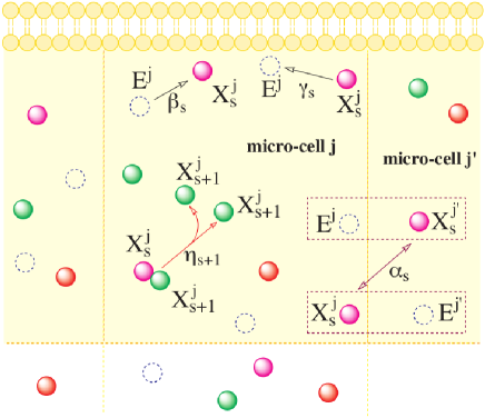
Figure 1: (Color online) The volume of the cells adjacent to the boundary is imagined to be partitioned into $\Omega$ micro-cells (see also Figure 2). Within micro-cell $j$ the molecular species interact according to the autocatalytic reactions specified by Eqs. (1). In addition, the molecules can migrate from micro-cell $j$ to its nearest neighbors, e.g. micro-cell $j^{\prime}$, as depicted in the cartoon. A molecule of type $X_{s}^{j}$ (full circle) takes over a vacancy (dashed empty circle) of micro-cell $E^{j^{\prime}}$, and so transforms into $X_{s}^{j^{\prime}}$, leaving behind a vacancy $E^{j}$. Finally, the chemical can also diffuse in from the environment, a reaction that in turn implies changing $E^{j}$ into $X_{s}^{j}$. The opposite holds for molecules that diffuse out into the environment.

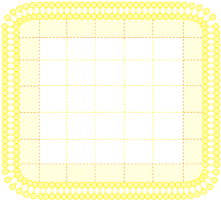
Figure 2: (Color online) In the spatial autocatalytic model considered here the vesicle is imagined to be divided into small micro-cells. We are specifically interested in the micro-cells adjoining the membrane, shown in darker outline in the figure. These latter link up together and constitute a sort of inner shell, immediately adjacent to the vesicle wall. Within each micro-cell the chemicals interact as shown in Figure 1.

In the following we will formulate the model in terms of a chemical master equation and find the mean-field solution as well as determining stochastic corrections to this which occurs when $N$ is finite. We will also simulate the stochastic dynamics and compare the results with the analytic formulas we obtain.

To describe the model as a chemical master equation, we denote the number of molecules of chemical species $s$ in cell $j$ by $n_{s}^{j}$, and so the state of the system can be characterized by the vector $\textbf{n}=(\textbf{n}^{1},\textbf{n}^{2},...,\textbf{n}^{\Omega})$ where $\textbf{n}^{j}=(n_{1}^{j},n_{2}^{j},...,n_{k}^{j})$. The transition rate from one state $\textbf{n}^{\prime}$, to another n, is denoted by $T(\textbf{n}|\textbf{n}^{\prime})$ — with the initial state being on the right. For example, the transitions stemming from the autocatalytic cycles are

$$T(n_{s}^{j}-1,n_{s+1}^{j}+1|n_{s}^{j},n_{s+1}^{j})=\frac{\eta_{s+1}}{\Omega}\frac{n_{s}^{j}}{N}\frac{n_{s+1}^{j}}{N},$$ (5)

where within the brackets we have chosen to indicate only the dependence on those species which are involved in the reaction. The transition rates associated with the migration between adjacent micro-cells take the form

$$T(n_{s}^{j}-1,n_{s}^{j^{\prime}}+1|n_{s}^{j},n_{k}^{j^{\prime}}) = \frac{\alpha_{s}}{z\Omega}\frac{n_{s}^{j}}{N}\Big{(}1-\sum_{m=1}^{k}\frac{n^{j^{\prime}}_{m}}{N}\Big{)},$$

$$T(n_{s}^{j}+1,n_{s}^{j^{\prime}}-1|n_{s}^{j},n_{s}^{j^{\prime}}) = \frac{\alpha_{s}}{z\Omega}\frac{n_{s}^{j^{\prime}}}{N}\Big{(}1-\sum_{m=1}^{k}\frac{n^{j}_{m}}{N}\Big{)},$$ (6)

where $z$ is the number of nearest neighbors that each micro-cell has. Finally, for the interaction with the environment, the transition rates are

$$T(n_{s}^{j}-1|n_{s}^{j})=\frac{\gamma_{s}}{\Omega}\frac{n_{s}^{j}}{N},$$

$$T(n_{s}^{j}+1|n_{s}^{j})=\frac{\beta_{s}}{\Omega}\Big{(}1-\sum_{m=1}^{k}\frac{n^{j}_{m}}{N}\Big{)}.$$ (7)

In Eqs. (6) and (7), explicit use has been made of the condition

$$\sum^{k}_{s=1}\frac{n^{j}_{s}}{N}+\frac{n^{j}_{E}}{N}=1,$$ (8)

to eliminate $n^{j}_{E}$, the number of vacancies in cell $j$.

The system is intrinsically stochastic and may be described by the probability density function, $P(\textbf{n},t)$, which gives the probability of finding the system in state n at time $t$. The equation which governs the dynamical evolution of $P(\textbf{n},t)$ is the master equation van07 , which for the system under consideration here takes the form

$$\frac{dP(\textbf{n},t)}{dt} = \sum^{\Omega}_{j=1}{\cal T}^{j}_{\rm loc}P(\textbf{n},t)+\sum^{\Omega}_{j=1}\sum_{j^{\prime}\in j}{\cal T}^{jj^{\prime}}_{\rm mig}P(\textbf{n},t)$$ (9)

$$+ \sum^{\Omega}_{j=1}{\cal T}^{j}_{\rm env}P(\textbf{n},t),$$

where the three terms on the right-hand side refer to the local terms for the chemical reactions, the migration of chemical species between the micro-cells, and the interaction with the environment, respectively. The notation $j^{\prime}\in j$ means that the cell $j^{\prime}$ is a nearest-neighbor of the cell $j$. The three terms in the master equation can be expressed in a concise, but transparent, form by introducing the step operator van07 ${\cal E}^{\pm 1}_{s,j}$ defined by

$${\cal E}^{\pm 1}_{s,j}f(\{n^{i}_{m}\})=f(\ldots,n^{j}_{s}\pm 1,\ldots),$$ (10)

where $f$ is an arbitrary function. The explicit forms for these three terms are

$${\cal T}^{j}_{\rm loc} = \sum^{k}_{s=1}\left({\cal E}_{s,j}{\cal E}^{-1}_{s+1,j}-1\right)T(n^{j}_{s}-1,n^{j}_{s+1}+1|n^{j}_{s},n^{j}_{s+1})$$

$${\cal T}^{jj^{\prime}}_{\rm mig} = \sum^{k}_{s=1}\left({\cal E}_{s,j}{\cal E}^{-1}_{s,j^{\prime}}-1\right)T(n^{j}_{s}-1,n^{j^{\prime}}_{s}+1|n^{j}_{s},n^{j^{\prime}}_{s})$$

$$+\sum^{k}_{s=1}\left({\cal E}_{s,j^{\prime}}{\cal E}^{-1}_{s,j}-1\right)T(n^{j^{\prime}}_{s}-1,n^{j}_{s}+1|n^{j^{\prime}}_{s},n^{j}_{s})$$

$${\cal T}^{j}_{\rm env} = \sum^{k}_{s=1}\left[\left({\cal E}_{s,j}-1\right)T(n^{j}_{s}-1|n^{j}_{s})\right.$$ (13)

$$+\left.\left({\cal E}^{-1}_{s,j}-1\right)T(n^{j}_{s}+1|n^{j}_{s})\right],$$

where it is understood that the operator ${\cal E}^{\pm 1}_{s,j}$ also acts on $P(\textbf{n},t)$ when these expressions are substituted into Eq. (9). In Eq. (LABEL:local) the cyclic nature of the reactions means that $n^{j}_{k+1}$ should be identified as $n^{j}_{1}$ and ${\cal E}^{\pm 1}_{k+1,j}$ should be identified as ${\cal E}^{\pm 1}_{1,j}$. The explicit expressions for the transition rates are given by Eqs. (5)-(7). These, together with Eqs. (9)-(13) define the model.

The above description is exact; no approximations have yet been made. At this stage we could also resort to direct numerical simulations of the chemical reaction system by use of the Gillespie algorithm gil76 ; gil77 . This method produces realizations of the stochastic dynamics which are formally equivalent to those found from the master equation (9). Averaging over many realizations enables us to calculate quantities of interest. We will discuss the results of performing such simulations in Section IV, but a very accurate approximation scheme exists which can be used to investigate models of this type analytically. This is the van Kampen system-size expansion van07 . It is effectively an expansion in powers of $N^{-1/2}$, which to leading order ($N\to\infty$) gives the deterministic equations describing the system, and which at next-to-leading order gives finite $N$ corrections to these. These latter corrections take the form of linear stochastic differential equations which can then be analyzed straightforwardly, especially in the case when the deterministic system has approached a stable fixed point. The method is based on substituting the ansatz

$$\frac{n_{s}^{j}}{N}=\phi_{s}^{j}+\frac{1}{\sqrt{N}}\xi_{s}^{j},$$ (14)

into the master equation (9). Here $\phi_{s}^{j}(t)$ is the solution to the deterministic equation, and $\xi_{s}^{j}(t)$ is a stochastic term which is the difference between the actual value $n_{s}^{j}/N$ and $\phi_{s}^{j}$ at time $t$.

We develop this approximation in the next two sections. In Section III we carry out the analysis to leading order, finding the deterministic equations and the relevant fixed point. In Section IV we carry through the calculation to next-to-leading order, investigating the linear stochastic differential equations by taking their Fourier transforms. The derivations of these equations is lengthy, though straightforward, and the details of the expansion are provided in Appendices A and B.

III Leading order: the deterministic equations

In the limit where the number of molecules (including vacancies) in each micro-cell, $N$, goes to infinity, the system becomes deterministic and is governed by a set of ordinary differential equations. These are found by substituting the ansatz (14) into the master equation (9) and letting $N\to\infty$, after the introduction of a rescaled time $\tau={t}/{(N\Omega)}$. The calculation is described in Appendix A, but the same equation can also be found by multiplying Eq. (9) by $n^{i}_{r}$ and summing over all states n. Either way one obtains the following equation for species $s$ in cell $j$

$$\frac{d\phi_{s}^{j}}{d\tau} = \eta_{s}\phi_{s-1}^{j}\phi_{s}^{j}-\eta_{s+1}\phi_{s}^{j}\phi_{s+1}^{j}$$ (15)

$$+ \alpha_{s}\Big{(}\Delta\phi_{s}^{j}(1-\sum_{m=1}^{k}\phi_{m}^{j})+\phi_{s}^{j}\sum_{m=1}^{k}\Delta\phi_{m}^{j}\Big{)}$$

$$+ \beta_{s}(1-\sum_{m=1}^{k}\phi_{m}^{j})-\gamma_{s}\phi_{s}^{j},$$

where $\Delta$ is the discrete Laplacian operator $\Delta f_{s}^{j}=(2/z)\sum_{j^{\prime}\in j}(f_{s}^{j^{\prime}}-f_{s}^{j})$. In the limit where the size of the micro-cells tends to zero, these equations become partial differential equations, with $\Delta$ becoming the familiar Laplacian operator. In this respect, Eq. (15) generalizes the results of dau09 to the case of a spatially-extended system. When turning off the migration mechanism between neighboring micro-cells, i.e. imposing $\alpha_{s}=0$ for any species $s$, the spatial aspects drop out and one formally recovers the ordinary differential equations given in dau09 .

To proceed with the analysis, and to make contact with the investigation carried out in tog01 ; dau09 , we shall now assign the same chemical parameters to all the species. The migration rate is the only exception to this, and may have a different value for each species. We will see later that this will be necessary in order to find spatio-temporal oscillations but also, as we will see shortly, a straightforward analysis is still possible if we maintain in $\alpha_{s}$, and none of the other parameters, an explicit reference to the index $s$. We will be concerned with finding the homogeneous solution of Eq. (15), that is, the solution with no spatial variation. The homogeneous solution is found to be an attractor of the deterministic dynamics, even when the system is initially prepared in a non-homogeneous configuration. This observation follows from numerical simulations, but can in principle be made quantitative by investigating the stability of the homogeneous fixed point. This means that no gradient in concentration is allowed between neighboring micro-cells, once the asymptotic regime is attained. So, when searching for fixed points of the dynamics, one can set the terms involving the Laplacian in Eq. (15) to zero. Since the only dependence on $s$, appearing in $\alpha_{s}$, multiplies these terms, there is also no dependence remaining on the species type, $s$, and so the fixed points are both independent of $j$ and of $s$. Under these conditions a unique fixed point for the concentration, $\phi^{*}$, is easily found to be

$$\phi^{*}=\frac{\beta}{k\beta+\gamma},$$ (16)

for any $s=1,...,k$ and $j=1,...,\Omega$. The result (16) is identical to that obtained in dau09 , when dealing with the non-spatial homologous model.

In dau09 , fluctuations for finite $N$ were shown to induce regular temporal oscillations in the species populations, so significantly altering the predicted deterministic dynamics. What is going to happen in the present spatial context? In Section IV we shall investigate this, the central point of the paper, by focusing on the next-to-leading order corrections in the van Kampen expansion.

IV Next-to-leading order: the stochastic corrections

Equating the terms of next-to-leading order in the master equation, after rescaling the time, leads to the Fokker-Planck equation (35) which governs the probability density function of the fluctuations. This Fokker-Planck equation is formally equivalent to the following Langevin equation gar04 ; ris89

$$\frac{d\xi^{j}_{s}}{d\tau}=\sum_{j^{\prime},r}M_{sr}^{jj^{\prime}}\xi^{j^{\prime}}_{r}+\lambda^{j}_{s}(\tau),$$ (17)

where

$$\langle\lambda_{s}^{j}(\tau)\lambda_{r}^{j^{\prime}}(\tau^{\prime})\rangle=\mathcal{B}_{sr}^{jj^{\prime}}\delta(\tau-\tau^{\prime}).$$ (18)

The noise term, $\lambda^{j}_{s}(\tau)$, in Eq. (17) is Gaussian with zero mean and with a correlator given by Eq. (18), from which it can be seen to be white. The form of the two matrices $M$ and $\mathcal{B}$ are discussed in Appendix B. They depend on the solution of the deterministic equation $\phi_{s}^{j}(\tau)$, and so in principle are time-dependent, since $\phi_{s}^{j}$ is. However, in practice we are interested in fluctuations about the stationary state, $\phi^{*}$, and so they lose their time dependence. They also only have a non-trivial spatial dependence through the presence of the discrete Laplacian, because the stationary state is homogeneous. Therefore the calculation can be considerably simplified by taking the spatial Fourier transform of Eqs. (17) and (18). As discussed in Appendix B this gives (see also lug08 )

$$\frac{d\xi^{\textbf{k}}_{s}}{d\tau}=\sum_{r}M_{sr}^{\textbf{k}}\xi^{\textbf{k}}_{r}+\lambda^{\textbf{k}}_{s}(\tau),$$ (19)

where

$$\langle\lambda_{s}^{\textbf{k}}(\tau)\lambda_{r}^{\textbf{k}^{\prime}}(\tau^{\prime})\rangle=\mathcal{B}_{sr}^{\textbf{k}}\Omega a^{d}\delta_{\textbf{k}+\textbf{k}^{\prime},0}\delta(\tau-\tau^{\prime}),$$ (20)

and where k is the wavevector. Here we have assumed that the micro-cells form a hypercubic lattice in $d-$dimensions with a lattice spacing $a$. The matrices $M^{\textbf{k}}$ and $\mathcal{B}^{\textbf{k}}$ are given by Eqs. (43)-(50) and Eqs. (52)-(59) respectively. However the important point is that now k is simply a label and the matrix structure originating from the spatial nature of the problem has been lost. Thus both $M^{\textbf{k}}$ and $\mathcal{B}^{\textbf{k}}$ are simply $k\times k$ matrices (recall that $k$ is the number of chemical species) and the analysis from now on is as in the non-spatial case dau09 .

As we have already stressed in this paper, fluctuations about the stationary state need to be taken into account, since they can be significant even if $N$ is quite large. The fact we can investigate these systematically is crucially dependent on the linearity of Eq. (19) and that the $M^{\textbf{k}}$ and $\mathcal{B}^{\textbf{k}}$ matrices are time-independent. It means that we can straightforwardly take the temporal Fourier transform of Eq. (19) to obtain

$$\sum^{k}_{r=1}\left(-i\omega\delta_{sr}-M_{sr}^{\textbf{k}}\right)\tilde{\xi}^{\textbf{k}}_{r}(\omega)=\tilde{\lambda}^{\textbf{k}}_{s}(\omega),$$ (21)

where $\tilde{f}$ denotes the temporal Fourier transform of the function $f$. Defining the matrix $(-i\omega\delta_{sr}-M_{sr}^{\textbf{k}})$ to be $\Phi^{\textbf{k}}_{sr}(\omega)$, the solution to Eq. (21) is

$$\tilde{\xi}^{\textbf{k}}_{r}(\omega)=\sum^{k}_{s=1}\left[\Phi^{\textbf{k}}(\omega)\right]^{-1}_{rs}\tilde{\lambda}^{\textbf{k}}_{s}(\omega).$$ (22)

From previous investigations, and the nature of the system, we expect that the fluctuations about the stationary state (16) will oscillate, and will also be sustained and enhanced by a resonant effect mck05 ; dau09 . This is indeed what is seen. To investigate this effect systematically we focus our attention on the power spectrum $P_{s}(\textbf{k},\omega)$ of the fluctuations of species $s$,

$$P_{s}(\textbf{k},\omega)\equiv\left\langle|\xi^{\textbf{k}}_{s}(\omega)|^{2}\right\rangle=$$

$$\Omega a^{d}\sum^{k}_{r=1}\sum^{k}_{u=1}\left[\Phi^{\textbf{k}}(\omega)\right]^{-1}_{sr}\mathcal{B}^{\textbf{k}}_{ru}\left[\Phi^{\textbf{k}\,{\dagger}}(\omega)\right]^{-1}_{us}.$$ (23)

The theoretical power spectrum can be found and plotted out, for any given choice of the chemical parameters, from Eq. (23). To make contact with earlier investigations dau09 , and aiming at elucidating the spatial effects, we here solely focus on the choice $k=4$ and select $\eta=10$, $\beta=5/32$, and $\gamma=5/32$. When the $\alpha_{s}$ are set equal to zero, the communication between neighboring micro-cells is silenced, each spatial block behaving as an independent unit. Based on Eq. (23), a temporal peak in the power spectrum is predicted to occur. The peak is approximately located at $\omega\simeq 4$, in agreement with the analysis developed in dau09 . Another simple limit is when the $\alpha_{s}$ are made equal for all of the $k$ chemical species. In this case, the temporal peak gets progressively damped at large k, the effect being more pronounced the larger the values for the migration parameters. A similar phenomenon was also reported to occur in lug08 .

More interestingly, in Fig. 3, we show the theoretical power spectrum Eq. (23) for $\alpha_{s}$ that take different values for each of the species in the case of a two-dimensional vesicle (a one-dimensional periodic lattice of micro-cells, i.e. $d=1$). The range of variation of the $\alpha_{s}$ covers several orders of magnitude, which in turn corresponds to assigning a significantly different degree of mobility to the species. Molecules characterized by large values of $\alpha_{s}$ will quickly diffuse, while those with smaller $\alpha_{s}$ are associated with relatively static, and presumably, more massive, species. A localized peak is clearly displayed suggesting that organized spatio-temporal patterns can spontaneously emerge, due to the inherent stochasticity of the system. From an inspection of Figs. 3, it is also evident that the power spectrum shows a clear peak for all four species. We found that making the $\alpha_{s}$ significantly different among species was a simple way to produce localized spatio-temporal patterns. We also found that they could be produced if (at least) one of the $\alpha_{s}$ was sufficiently large, when compared with the others.

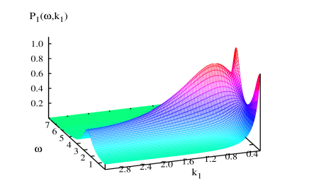
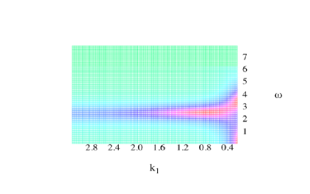
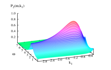
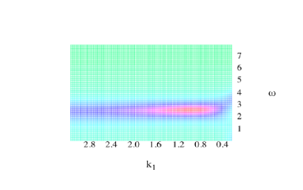
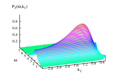
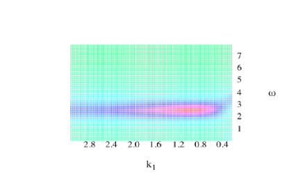
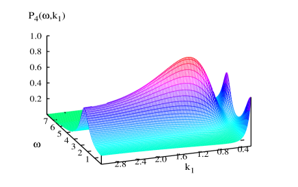
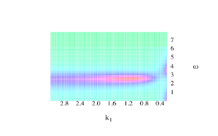
Figure 3: (Color online) Power spectra calculated from Eq. (23) for $k=4$ species and for a two-dimensional vesicle (one-dimensional periodic array of micro-cells). Here $N=5000$, $\Omega=256$, $\eta=10$, $\beta=5/32$, $\gamma=5/32$ and $\boldsymbol{\alpha}=[100,0.001,1,500]$. Each pair of panels (the three-dimensional plot and its two-dimensional projection) refers to a different chemical species. A localized peak is displayed predicting the existence of regular spatio-temporal patterns.

The conclusion of the above analysis, as well as the accuracy of the approximations that have been employed, can be tested via direct numerical simulations. By averaging over many realizations, we can calculate the power spectra after Fourier transformation. Results of the simulation are displayed in Fig. 4 for the same choice of parameters as in Fig. 3. The correspondence between the profiles is excellent and so confirms the correctness of our theoretical scheme.

In summary, we have unambiguously demonstrated that organized spatio-temporal cycles can emerge in a simple model of protocells where the constituents inside the vesicle interact via an autocatalytic scheme. As we shall argue in the following, this finding provides a possible mechanism to drive a dynamical synchronization between the duplication of genetic material inside a protocell and the division of the vesicle membrane.

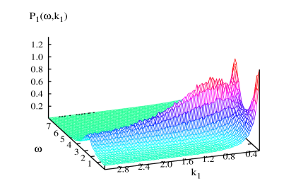
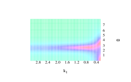
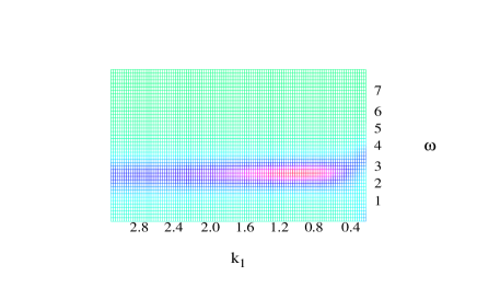
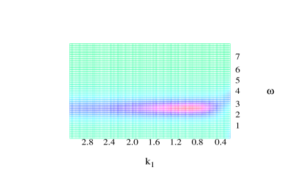
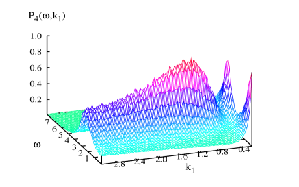
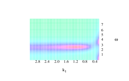
Figure 4: (Color online) Numerically calculated power spectra obtained from averaging 800 realizations. Stochastic simulations are performed via the Gillespie algorithm. Parameters are set as in Fig. 3.

V Discussion

In this paper we have investigated how the discreteness of the constituents in an autocatalytic chemical reaction can lead to spatio-temporal oscillations. The occurrence of temporal oscillations in such a setting, but without a spatial element, has previously been studied tog01 ; dau09 . Similarly, such oscillations have been studied for a predator-prey system in a spatial framework lug08 , but the oscillations in this case did not occur at a non-zero value of k. In this paper, we have combined and generalized these treatments, and also put them into the context of vesicles, which suggests an interesting consequence of the oscillatory behavior.

We can speculate that the natural tendency of the chemical constituents to organize in regular spatio-temporal cycles can be instrumental in achieving a degree of synchronization between the outer membrane of the vesicle and the mixture of chemicals inside. In the context of protocells, these chemicals undergoing autocatalytic reactions are to be interpreted as a primitive form of genetic material. One would expect, as a minimal self-consistency requirement, that within a stable population, a vesicle would split into two when the chemical material contained within it had approximately doubled in size. It is tempting to postulate that such a property is a dynamical phenomenon, the density fluctuations acting as a positive feedback on the vesicle growth, so signaling when the constituents inside the vesicle are ready for the splitting to take place.

Now let us imagine that the vesicle containing the chemical species grows, because of the inclusion of successive membrane constituents from the environment in which it moves. Laboratory experiments indicate lui06 that a vesicle filled with water or solutes is kept in a turgid spherical shape while growing by additional material of a similar kind flowing in from the outside environment. It is believed that the vesicle remains spherical until a thermodynamic instability sets in which distorts the structure fan08 , eventually leading to fissioning. Now suppose that the vesicle is filled by a discrete population of chemical constituents, which undergo an independent dynamics of the autocatalytic type. As illustrated in this paper, the chemicals experience a first rapid evolution towards the stationary state, where enhanced oscillations appear due to the intrinsic finiteness of the interacting constituents. Such oscillations might seed an instability mac07a ; mac07b , which could resonate with the innate ability of the container to divide, so initiating the splitting process. These ideas could be extended to protocells, where enhanced oscillations could originate in the primitive genetic material. These oscillations could signal to the membrane that the genetic evolution had been virtually taken to completion and that the fission could now occur, so ensuring that the genetic material is passed on to the daughter protocells. This is a highly speculative suggestion, which calls for further investigation in the context of self-consistent formulations, where both the membrane and the genetic material are dynamically evolved.

It is clear that the work presented here can be extended in various ways. The nature of the lattice structure that is assumed can be generalized. For instance it is straightforward to include next-nearest neighbors, next-next nearest neighbor and so on. The analytical treatment is analogous, and the results the same; only the form of the operator $\Delta_{\textbf{k}}$ changes. Numerical simulations could also be performed in higher dimensions. In particular, a toroidal (donut-like) cell embedded in a three-dimensional space can be straightforwardly simulated. The inner volume of the cell is again partitioned into micro-cells, and distinct diffusion rates are assigned to the radial and longitudinal directions. Preliminary simulations indicate that collective modes can develop giving rise to organized spatio-temporal dynamics dipa10 .

Appendix A The van-Kampen expansion

In this Appendix we will give more details of the application of the van Kampen system-size expansion to the master equation (9). A general discussion of the method is given in van Kampen’s book van07 and a description of the application to a simple model showing sustained and enhanced stochastic fluctuations is given in mck05 . The calculations given below build upon those carried out for the non-spatial version of the model considered in this paper dau09 and a spatial predator-prey model lug08 . We will occasionally refer back to these two papers below.

The starting point for the expansion in powers of $N^{-1/2}$ is the ansatz (14). From this the following two results can be derived van07 . First, the left-hand side of the master equation (9) is given by

$$\frac{dP(\textbf{n},t)}{dt}=\frac{\partial\Pi(\xi_{m}^{i},t)}{\partial t}-N^{\frac{1}{2}}\sum_{j=1}^{\Omega}\sum_{s=1}^{k}\frac{\partial\Pi(\xi_{m}^{i},t)}{\partial\xi_{s}^{j}}\frac{d\phi_{s}^{j}}{dt},$$ (24)

where $\Pi(\xi_{m}^{i},t)\equiv P(n_{m}^{i},t)$. Second, the step operator ${\cal E}^{\pm 1}_{s,j}$ may be expanded:

$${\cal E}^{\pm 1}_{s,j} = 1\pm N^{-\frac{1}{2}}\frac{\partial}{\partial\xi_{s}^{j}}+(2N)^{-1}\frac{\partial^{2}}{\partial(\xi_{s}^{j})^{2}}+\ldots$$ (25)

$$\equiv 1\pm N^{-\frac{1}{2}}\partial_{\xi_{s}^{j}}+(2N)^{-1}\partial^{2}_{\xi_{s}^{j}}+\ldots.$$

The right-hand side of the master equation may be also expanded. We begin by defining new operators which are the coefficients of $N^{-1/2}$ and $N^{-1}$ in the expansion of the particular combinations of the step operators which appear in the model. These are

$$({\cal E}_{s,j}{\cal E}_{s+1,j}^{-1}-1)\simeq N^{-\frac{1}{2}}\Big{(}\partial_{\xi_{s}^{j}}-\partial_{\xi_{s+1}^{j}}\Big{)}$$

$$+\frac{1}{2}\Big{[}N^{-\frac{1}{2}}\Big{(}\partial_{\xi_{s}^{j}}-\partial_{\xi_{s+1}^{j}}\Big{)}\Big{]}^{2}\equiv N^{-\frac{1}{2}}\widehat{L}_{1s}+\frac{1}{2}N^{-1}\widehat{L}_{2s},$$

$$({\cal E}_{s,j}{\cal E}_{s,j^{\prime}}^{-1}-1)\simeq N^{-\frac{1}{2}}\Big{(}\partial_{\xi_{s}^{j}}-\partial_{\xi_{s}^{j^{\prime}}}\Big{)}$$

$$+\frac{1}{2}\Big{[}N^{-\frac{1}{2}}\Big{(}\partial_{\xi_{s}^{j}}-\partial_{\xi_{s}^{j^{\prime}}}\Big{)}\Big{]}^{2}\equiv N^{-\frac{1}{2}}\widehat{L}_{1j}+\frac{1}{2}N^{-1}\widehat{L}_{2j},$$

where the operators $\widehat{L}_{1s}$ and $\widehat{L}_{2s}$ read

$$\widehat{L}_{1s}=\Big{(}\partial_{\xi_{s}^{j}}-\partial_{\xi_{s+1}^{j}}\Big{)},\ \ \widehat{L}_{2s}=\Big{(}\partial_{\xi_{s}^{j}}-\partial_{\xi_{s+1}^{j}}\Big{)}^{2},$$

and where $\widehat{L}_{1j}$ and $\widehat{L}_{2j}$ read

$$\widehat{L}_{1j}=\Big{(}\partial_{\xi_{s}^{j}}-\partial_{\xi_{s}^{j^{\prime}}}\Big{)},\ \ \widehat{L}_{2j}=\Big{(}\partial_{\xi_{s}^{j}}-\partial_{\xi_{s}^{j^{\prime}}}\Big{)}^{2}.$$

In addition

$$({\cal E}_{s,j}^{-1}-1)\sim-N^{-\frac{1}{2}}\ \partial_{\xi_{s}^{j}}+\frac{1}{2}N^{-1}\partial^{2}_{\xi_{s}^{j}},$$

$$({\cal E}_{s,j}-1)\sim N^{-\frac{1}{2}}\ \partial_{\xi_{s}^{j}}+\frac{1}{2}N^{-1}\partial^{2}_{\xi_{s}^{j}}.$$

For each of the three terms appearing in Eq. (9), namely the local, migration and environmental terms, we can now identify the various contributions in the van Kampen expansion: those of order $N^{-1/2}$, those of order $N^{-1}$ involving a single derivative, and those of order $N^{-1}$ but involving two derivatives. We will examine these in turn.

A.1 Right-hand side of the master equation: the $N^{-1/2}$ terms

The contribution from ${\cal T}^{j}_{\rm loc}$, defined by Eq. (LABEL:local), is

$$\sum_{s}\frac{\eta_{s+1}}{\Omega}\widehat{L}_{1s}(\phi_{s}^{j}\phi_{s+1}^{j}).$$

Using the definition of $\widehat{L}_{1s}$, shifting the sum on $s$ and remembering that quantities with subscripts $k+1$ are to be identified with those with subscripts $1$, we obtain

$${\cal T}^{j(1)}_{\rm loc}=\frac{1}{\Omega}\sum_{s}(\eta_{s+1}\phi_{s}^{j}\phi_{s+1}^{j}-\eta_{s}\phi_{s-1}^{j}\phi_{s}^{j})\partial_{\xi_{s}^{j}},$$ (26)

where the superscript $(1)$ indicates that this is only the contribution to ${\cal T}^{j}_{\rm loc}$ from terms of order $N^{-1/2}$. It should be noted that Eq. (26) operates on $\Pi(\xi_{m}^{i},t)$.

The contribution from ${\cal T}^{jj^{\prime}}_{\rm mig}$, defined by Eq. (LABEL:migration) and using the definition of $\widehat{L}_{1j}$, is

$$\frac{2}{z\Omega}\sum_{s}\alpha_{s}\partial_{\xi_{s}^{j}}\left(\phi_{s}^{j}(1-\sum_{m}\phi_{m}^{j^{\prime}})-\phi_{s}^{j^{\prime}}(1-\sum_{m}\phi_{m}^{j})\right).$$

To write this contribution in a way which naturally involves the Laplacian operator we add to this sum two terms which add to zero, namely

$$0=\phi_{s}^{j}\sum_{m}\phi_{m}^{j}-\phi_{s}^{j}\sum_{m}\phi_{m}^{j}.$$

Summing the contribution over $j^{\prime}\in j$ and introducing the discrete Laplacian $\Delta f_{s}^{j}=(2/z)\sum_{j^{\prime}\in j}(f_{s}^{j^{\prime}}-f_{s}^{j})$ we obtain

$$\sum_{j^{\prime}}{\cal T}^{jj^{\prime}(1)}_{\rm mig}=-\sum_{s}\frac{\alpha_{s}}{\Omega}\Big{(}\Delta\phi_{s}^{j}(1-\sum_{m}\phi_{m}^{j})+\phi_{s}^{j}\sum_{m}\Delta\phi_{m}^{j}\Big{)}.$$ (27)

The contribution from ${\cal T}^{j}_{\rm env}$, defined by Eq. (13), is immediately found to be

$${\cal T}^{j(1)}_{\rm env}=\sum_{s}\Big{[}\frac{\partial}{\partial\xi_{s}^{j}}\Big{(}\frac{\gamma_{s}}{\Omega}\phi_{s}^{j}-\frac{\beta_{s}}{\Omega}(1-\sum_{m}\phi_{m}^{j})\Big{)}\Big{]}.$$ (28)

Adding the three terms (26)-(28) together, and letting them act on $\Pi(\xi_{m}^{i},t)$ and summing over $j$, we may equate the resulting expression to the order $N^{1/2}$ term in Eq. (24), after the rescaling of time $\tau=t/(N\Omega)$. The resulting equation describes the deterministic time-evolution of the species $s$ in micro-cell $j$ in the limit $N\to\infty$, and is given by Eq. (15) in the main text.

A.2 Right-hand side of the master equation: the $N^{-1}$ terms with a single derivative

These contributions are expressed in terms of the operators $\widehat{L}_{1s}$ and $\widehat{L}_{1j}$, and so are a function of the first derivatives in the fluctuation variables. We proceed as we did for the terms of order $N^{-1/2}$.

The contribution from ${\cal T}^{j}_{\rm loc}$, defined by Eq. (LABEL:local), is

$${\cal T}^{j(2)}_{\rm loc}=\sum_{s=1}^{k}\frac{\eta_{s+1}}{\Omega}\Big{[}\widehat{L}_{1s}\Big{(}\phi_{s}^{j}\xi_{s+1}^{j}+\phi_{s+1}^{j}\xi_{s}^{j}\Big{)}\Big{]}$$ (29)

$$= \frac{1}{\Omega}\sum_{s=1}^{k}\Big{[}\frac{\partial}{\partial\xi_{s}^{j}}\Big{(}\phi_{s}^{j}(\eta_{s+1}\xi_{s+1}^{j}-\eta_{s}\xi_{s-1}^{j})$$

$$+ \xi_{s}^{j}(\eta_{s+1}\phi_{s+1}^{j}-\eta_{s}\phi_{s-1}^{j})\Big{)}\Big{]},$$

where once again use has been made of the definition $\widehat{L}_{1s}$, the cyclic nature of the species, and the sum on $s$ has been shifted. Here the superscript $(2)$ indicates that this is only the contribution to ${\cal T}^{j}_{\rm loc}$ from terms of order $N^{-1}$ with a single derivative.

The contribution from ${\cal T}^{jj^{\prime}}_{\rm mig}$, defined by Eq. (LABEL:migration), is

$$\frac{2}{z\Omega}\sum_{s}\alpha_{s}\Big{[}\widehat{L}_{1j}\Big{(}\phi_{s}^{j}(-\sum_{m}\xi_{m}^{j^{\prime}})+\xi_{s}^{j}(1-\sum_{m}\phi_{m}^{j^{\prime}})\Big{)}\Big{]}.$$

Performing the same manipulations as before, but also inserting the identities

$$0=\xi_{s}^{j}\sum_{m}\phi_{m}^{j}-\xi_{s}^{j}\sum_{m}\phi_{m}^{j},\ \ 0=\phi_{s}^{j}\sum_{m}\xi_{m}^{j}-\phi_{s}^{j}\sum_{m}\xi_{m}^{j},$$

gives, after summing over $j^{\prime}\in j$,

$$\sum_{j^{\prime}}{\cal T}^{jj^{\prime}(2)}_{\rm mig}=-\frac{1}{\Omega}\sum_{s}\alpha_{s}\Big{[}\frac{\partial}{\partial\xi_{s}^{j}}\Big{(}\Delta\xi_{s}^{j}+\xi_{s}^{j}\sum_{m}\Delta\phi_{m}^{j}$$ (30)

$$- \Delta\phi_{s}^{j}\sum_{m}\xi_{m}^{j}+\phi_{s}^{j}\sum_{m}\Delta\xi_{m}^{j}-\Delta\xi_{s}^{j}\sum_{m}\phi_{m}^{j}\Big{)}\Big{]}.$$

Finally, the contribution from ${\cal T}^{j}_{\rm env}$, defined by Eq. (13), is immediately found to be

$${\cal T}^{j(2)}_{\rm env}=\sum_{s}\Big{[}\frac{\partial}{\partial\xi_{s}^{j}}\Big{(}\frac{\gamma_{s}}{\Omega}\xi_{s}^{j}+\frac{\beta_{s}}{\Omega}\sum_{m}\xi_{m}^{j}\Big{)}\Big{]}.$$ (31)

A.3 Right-hand side of the master equation: the $N^{-1}$ terms with two derivatives

These terms are expressed in terms of the operator $\widehat{L}_{2s}$ and $\widehat{L}_{2j}$, and so are a function of the second order derivatives in the fluctuation variables. We proceed as we did in the two previous cases.

The contribution from ${\cal T}^{j}_{\rm loc}$ is

$${\cal T}^{j(3)}_{\rm loc}=\frac{1}{\Omega}\sum_{s}\eta_{s+1}\frac{1}{2}\widehat{L}_{2s}(\phi_{s}^{j}\phi_{s+1}^{j})$$ (32)

$$= \frac{1}{2\Omega}\sum_{s}\eta_{s+1}(\phi_{s}^{j}\phi_{s+1}^{j})\Big{(}\frac{\partial^{2}}{\partial(\xi_{s}^{j})^{2}}$$

$$+\frac{\partial^{2}}{\partial(\xi_{s+1}^{j})^{2}}-2\frac{\partial^{2}}{\partial\xi_{s}^{j}\partial\xi_{s+1}^{j}}\Big{)}.$$

The contribution from ${\cal T}^{jj^{\prime}}_{\rm mig}$ is

$${\cal T}^{jj^{\prime}(3)}_{\rm mig}=\frac{1}{z\Omega}\sum_{s}\alpha_{s}\frac{1}{2}\Big{[}\widehat{L}_{2j}(\phi_{s}^{j}(1-\sum_{m}\phi_{m}^{j^{\prime}}))\Big{]}=$$

$$\alpha_{s}\frac{1}{z\Omega}\sum_{s}\Big{(}\phi_{s}^{j}(1-\sum_{m}\phi_{m}^{j^{\prime}})\Big{)}\Big{[}\frac{\partial}{\partial\xi_{s}^{j}}-\frac{\partial}{\partial\xi_{s}^{j^{\prime}}}\Big{]}^{2}.$$ (33)

Finally, the contribution from ${\cal T}^{j}_{\rm env}$ is found to be

$${\cal T}^{j(3)}_{\rm env}=\frac{1}{2}\sum_{s}\Big{(}\frac{\beta_{s}}{\Omega}(1-\sum_{m}\phi_{m}^{j})+\frac{\gamma_{s}}{\Omega}\phi_{s}^{j}\Big{)}\frac{\partial^{2}}{\partial(\xi_{s}^{j})^{2}}.$$ (34)

Adding the six terms (29)-(34) together, and letting them act on $\Pi(\xi_{m}^{i},t)$ and summing over $j$, we may equate the resulting expression to the order one term in Eq. (24), after the rescaling of time $\tau=t/(N\Omega)$. The resulting equation gives the stochastic time-evolution of the species $s$ in micro-cell $j$. It takes the form of a Fokker-Planck equation which we now examine.

Appendix B The form of the matrices $M$ and $\mathcal{B}$

To write down the differential equation for $\Pi(\xi_{s}^{j},\tau)$, it is convenient to combine the indices $s$ and $j$, labeling the species and micro-cells respectively, by a single index $p$. To do this we imagine the $k\Omega$-dimensional vector with components $\xi_{s}^{j}$ as an ordered sequence of $\Omega$ vectors, each of $k$ components. This can be achieved by defining $p=(j-1)k+s$, so that the component $\xi_{p}$ represents the fluctuations associated with the $s$-th species in the $j$-th micro-cell.

Now the terms in Eqs. (29)-(31) take the form of a single derivative of $\xi_{p}$ acting on a linear combination of $\xi_{l}$, $l=1,\ldots,k\Omega$ and the terms in Eqs. (32)-(34) are a linear combination of second order derivatives. Therefore using this more compact notation the Fokker-Planck takes the form

$$\frac{\partial\Pi}{\partial\tau} = -\sum_{p}\frac{\partial}{\partial\xi_{p}}\Big{[}\mathcal{A}_{p}(\boldsymbol{\xi})\Pi\Big{]}+\frac{1}{2}\sum_{l,p}\mathcal{B}_{lp}\frac{\partial^{2}\Pi}{\partial\xi_{l}\partial\xi_{p}},$$

(35)

where the matrix $\mathcal{A}$ can be re-written as

$$\mathcal{A}_{p}(\boldsymbol{\xi})=\sum_{l}M_{pl}\xi_{l}.$$ (36)

So to specify the Fokker-Planck equation we need to give the form of the two $(k\Omega)\times(k\Omega)$ matrices $M$ and $\mathcal{B}$. We first note that although they do not depend on the fluctuations $\xi_{p}(\tau)$, they do depend on the solution of the deterministic differential equation (15), as well as on the reaction rates $\eta_{s},\alpha_{s},\beta_{s}$ and $\gamma_{s}$. However since we are only interested in the fluctuations about the stationary state $\phi^{*}$ given by Eq, (16), and since we obtained this solution under the assumption that $\eta_{s},\beta_{s}$ and $\gamma_{s}$ were independent of $s$, we take the two matrices to only depend on $\phi^{*},\eta,\beta,\gamma$ and $\alpha_{s}$. An inspection of Eqs. (29)-(34) reveals that the only spatial dependence in $M$ and $\mathcal{B}$ originates from the discrete Laplacian. This suggests that if we introduce spatial Fourier transforms, we should be able to diagonalize $M$ and $\mathcal{B}$, and so be left with matrices only in the species space. This is most easily carried out by not continuing to work with the Fokker-Planck equation (35), but instead with the equivalent Langevin equation gar04 ; ris89

$$\frac{d\xi_{p}}{d\tau}=\mathcal{A}_{p}(\boldsymbol{\xi})+\lambda_{p}(\tau),$$ (37)

where

$$\langle\lambda_{p}(\tau)\lambda_{q}(\tau^{\prime})=\mathcal{B}_{pq}\delta(\tau-\tau^{\prime}),$$ (38)

and where the noise term, $\lambda_{p}(\tau)$, in Eq. (37) is Gaussian with zero mean. This is Eq. (17) in the main text, but using the single index notation.

We follow the conventions and methods of lug08 for the spatial Fourier transforms. For simplicity, we shall assume that the lattice is a $d-$dimensional hypercubic lattice, with lattice spacing $a$. Then the Fourier transform, $f_{s}^{\bf k}$, of a function $f_{s}^{\bf j}$, is defined by

$$f_{s}^{\bf k}=a^{d}\sum_{\bf j}e^{-i{\bf k}.a{\bf j}}\,f_{s}^{\bf j},$$ (39)

where we have now written the lattice site label ${\bf j}$ as a vector to emphasize the $d-$dimensional nature of the transform. We may now take the spatial Fourier transform of the matrix $M$. Since the only spatial dependence is through the discrete Laplacian, we may decompose Eq. (36) as follows:

$$A^{\textbf{j}}_{s}=\sum_{\textbf{j}^{\prime}}\sum_{r}M^{\textbf{jj}^{\prime}}_{sr}\xi^{\textbf{j}^{\prime}}_{r}=\sum_{r}\left[M^{(NS)}_{sr}\xi^{\textbf{j}}_{r}+M^{(SP)}_{sr}\Delta\xi^{\textbf{j}}_{r}\right],$$ (40)

where the two $k\times k$ matrices $M^{(NS)}$ and $M^{(SP)}$ will be specified below. It is now straightforward to take the spatial Fourier transform of Eq. (40) to obtain lug08

$$A^{\textbf{k}}_{s}=\sum_{r}\left[M^{(NS)}_{sr}+M^{(SP)}_{sr}\Delta_{\textbf{k}}\right]\xi^{{\textbf{k}}}_{r},$$ (41)

where $\Delta_{\textbf{k}}$ is the Fourier transform of the discrete Laplacian and is given by

$$\Delta_{\textbf{k}}=\frac{2}{d}\sum_{\gamma=1}^{d}\left[\cos(\textrm{k}_{\gamma}a)-1\right].$$ (42)

Care should be taken not to confuse the components of the wavevector k, and $k$, the number of chemical species. We have denoted the $\gamma$-th component of the wave vector k by $\textrm{k}_{\gamma}$ to help avoid this confusion.

The quantity within the square brackets in Eq. (41) is the spatial Fourier transform of the matrix $M$. It is diagonal in $\textbf{k}-$space and so depends on the single label k. We may therefore write it as

$$M^{\textbf{k}}_{sr}=M^{(NS)}_{sr}+M^{(SP)}_{sr}\Delta_{\textbf{k}},$$ (43)

where the two matrices $M^{(NS)}$ and $M^{(SP)}$ may be read off from Eqs. (29)-(31), and are given by

$$M^{(NS)}_{ss}=-\beta-\gamma$$ (44)

$$M^{(NS)}_{sr}=\left\{\begin{array}[]{ll}-\eta\phi^{*}-\beta,&\qquad\textrm{if }r=s+1\\ \eta\phi^{*}-\beta,&\qquad\textrm{if }r=s-1\\ -\beta,&\qquad\textrm{if }|s-r|>1,\end{array}\right.$$ (48)

and

$$M^{(SP)}_{ss}=\alpha_{s}\left[1+(1-k)\phi^{*}\right]$$ (49)

$$M^{(SP)}_{sr}=\alpha_{s}\phi^{*}\ \ \textrm{if}\ s\neq r.$$ (50)

The matrix $M^{(NP)}$ is exactly the one found in the non-spatial version of the model dau09 , which is why we have attached the label ‘$NS$’ to it to signify the non-spatial contribution to $M$. The spatial, or ‘$SP$’, contribution is simply $M^{(SP)}\Delta_{\textbf{k}}$.

To take the Fourier transform of the matrix $\mathcal{B}$, we note that out of the three terms — given by Eqs. (32)-(34) — from which this matrix is constructed, the only non-trivial spatial dependence comes from Eq. (33). We display the contribution containing this dependence by noting the following relation:

$$\sum_{\textbf{j}}\sum_{\textbf{j}^{\prime}\in\textbf{j}}\Big{[}\frac{\partial}{\partial\xi_{s}^{\textbf{j}}}-\frac{\partial}{\partial\xi_{s}^{\textbf{j}^{\prime}}}\Big{]}^{2}=$$

$$2\sum_{\textbf{j}}\sum_{\textbf{j}^{\prime}}\Big{[}z\frac{\partial^{2}}{\partial(\xi_{s}^{\textbf{j}})^{2}}\delta_{\textbf{jj}^{\prime}}-\frac{\partial^{2}}{\partial\xi_{s}^{\textbf{j}}\partial\xi_{s}^{\textbf{j}^{\prime}}}J_{<\textbf{jj}^{\prime}>}\Big{]},$$ (51)

where $J_{<\textbf{jj}^{\prime}>}$ is equal to $1$ if $\textbf{j}^{\prime}$ and j are nearest neighbors, and zero otherwise. The part of the $\mathcal{B}$ matrix corresponding to the expression (51) is $(2z\delta_{\textbf{jj}^{\prime}}-2J_{<\textbf{jj}^{\prime}>})$ which has Fourier transform

$$a^{d}\left[2z-4\sum_{\gamma=1}^{d}\cos(\textrm{k}_{\gamma}a)\right]=-za^{d}\Delta_{\textbf{k}},$$

using Eq. (42) and $z=2d$. Therefore we may express the matrix $\mathcal{B}$ in Fourier space in a similar way to Eq. (43):

$$\mathcal{B}^{\textbf{k}}_{sr}=\mathcal{B}^{(NS)}_{sr}+\mathcal{B}^{(SP)}_{sr}\Delta_{\textbf{k}},$$ (52)

where the two $k\times k$ matrices $\mathcal{B}^{(NS)}$ and $\mathcal{B}^{(SP)}$ may be read off from Eqs. (32)-(34), and are given by

$$\mathcal{B}^{(NS)}_{ss}=a^{d}\left[\beta(1-k\phi^{*})+\gamma\phi^{*}+2\eta\left(\phi^{*}\right)^{2}\right]$$ (53)

$$\mathcal{B}^{(NS)}_{sr}=\left\{\begin{array}[]{ll}-a^{d}\eta\left(\phi^{*}\right)^{2},&\qquad\textrm{if }r=s+1\\ -a^{d}\eta\left(\phi^{*}\right)^{2},&\qquad\textrm{if }r=s-1\\ 0&\qquad\textrm{if }|s-r|>1,\end{array}\right.$$ (57)

and

$$\mathcal{B}^{(SP)}_{ss}=-2a^{d}\alpha_{s}\phi^{*}\left(1-k\phi^{*}\right)$$ (58)

$$\mathcal{B}^{(SP)}_{sr}=0\ \ \textrm{if}\ s\neq r.$$ (59)

Once again, the matrix $\mathcal{B}^{(NS)}$ is exactly the one found in the non-spatial version of the model dau09 , up to a factor of $a^{d}$, which is why we have attached the label ‘$NS$’ to it. The spatial contribution is $\mathcal{B}^{(SP)}\Delta_{\textbf{k}}$.

References

- (1) B. Alberts et al. Molecular Biology of the Cell, (Garland Science, New York, 2007). Fifth edition.
- (2) D. W. Deamer. Orig. Life Evol. Biosph. 17, 3 (1986).
- (3) H. J. Morowitz, B. Heinz, and D. W. Deamer. Orig. Life Evol. Biosph. 18, 281 (1988).
- (4) G. Ourisson and Y. Nakatani. Tetrahedron 55, 3183 (1999).
- (5) J. W. Szostak, D. P. Bartel and P. L. Luisi. Nature 409, 387 (2001).
- (6) S. Rasmussen et al. Science 303, 963 (2004).
- (7) I. A. Chen, R. W. Roberts, and J. W. Szostak. Science 305, 1474 (2004).
- (8) P. Stano and P. L. Luisi. Orig. Life Evol. Biosph. 37, 303 (2007).
- (9) D. Deamer. Prog. Theor. Phys. (Suppl) 173, 11 (2008).
- (10) S. Rasmussen et al. Protocells: Bridging nonliving and living matter, (MIT Press, Cambridge MA, 2008).
- (11) P. L. Luisi. The Emergence of Life, (Cambridge University Press, Cambridge, 2006).
- (12) U. Seifert. Adv. Phys. 46, 13 (1997).
- (13) P. Gray and S. K. Scott. J. Phys. Chem. 89, 22 (1985).
- (14) F. Dyson. Origins of Life (Cambridge University Press, Cambridge, England, 1985).
- (15) S. A. Kauffman. J. Theor. Biol. 119, 1 (1986); The Origins of Order (Oxford University Press, Oxford, 1993).
- (16) P. F. Stadler and P. Schuster, Bull. Math. Biol. 52, 485 (1990).
- (17) G. Wächtershäuser. Proc. Natl. Acad. Sci. U.S.A. 87, 200 (1990).
- (18) S. Jain and S. Krishna. Phys. Rev. Lett. 81, 5684 (1998).
- (19) M. Eigen. Naturwissenschaften 58, 465 (1971).
- (20) H. Lodish et al. Molecular Cell Biology (W. H. Freeman and Co., New York, 2008). Sixth edition.
- (21) Y. Togashi and K. Kaneko. Phys. Rev. Lett. 86, 2459 (2001).
- (22) Y. Togashi and K. Kaneko. J. Phys. Soc. Jpn. 72, 62 (2003).
- (23) T. Dauxois, F. Di Patti, D. Fanelli, and A. J. McKane. Phys. Rev. E 79, 036112 (2009).
- (24) N. G. van Kampen. Stochastic Processes in Physics and Chemistry (Elsevier, Amsterdam, 2007). Third edition.
- (25) A. J. McKane and T. J. Newman. Phys. Rev. Lett. 94, 218102 (2005).
- (26) A. J. McKane, J. D. Nagy, T. J. Newman, and M. O. Stefanini. J. Stat. Phys. 128, 165 (2007).
- (27) D. Alonso, A. J. McKane, and M. Pascual. J. R. Soc. Interface 4, 575 (2007).
- (28) C. A. Lugo and A. J. McKane. Phys. Rev. E 78, 051911 (2008).
- (29) D. T. Gillespie. J. Comput. Phys. 22, 403 (1976).
- (30) D. T. Gillespie. J. Phys. Chem. 81, 2340 (1977).
- (31) C. W. Gardiner. Handbook of Stochastic Methods (Springer-Verlag, Berlin, 2004). Third edition.
- (32) H. Risken. The Fokker-Planck Equation (Springer-Verlag, Berlin, 1989). Second edition.
- (33) D. Fanelli and A. J. McKane. Phys. Rev. E 78, 051406 (2008).
- (34) J. Macia and R. V. Solé, J. Theor. Biol. 245, 400 (2007).
- (35) J. Macia and R. V. Solé, Philos. Trans. R. Soc. London, Ser. B 362, 1821 (2007).
- (36) F. Di Patti, T. Dauxois, P. de Anna, D. Fanelli, and A. J. McKane. HCP-Europa 2, Final Report (2010).