IPPP/10/05 Resonant particle production at hadron colliders

Abstract:

We present a method to compute off-shell effects for processes involving resonant particles at hadron colliders with the possibility to include realistic cuts on the decay products. The method is based on an effective theory approach to unstable particle production and, as an example, is applied to $t$-channel single top production at the LHC.

1 Introduction

Heavy unstable particles such as the top quark, $Z$ and $W$ bosons as well as virtually all hypothetical particles in beyond-the-Standard-Model scenarios can only be studied through their decay products. The simplest way to compute cross sections involving such particles is to first consider on-shell production of the heavy particle and then its subsequent decay. Taking into account the matrix element of the decay of the on-shell particle — this is sometimes called the improved narrow-width approximation — it is possible to apply realistic cuts on the decay products. In this framework we can go to higher orders in perturbation theory by computing separately corrections to the production and the decay of the on-shell heavy particle. While this approximation is very often good enough, this talk addresses the question on how to go beyond and include off-shell effects in a systematic way. Thus we are led to consider processes with resonant (nearly on-shell) rather than on-shell heavy particles.

Even though the framework for computing off-shell effects presented here is quite general, let us consider an explicit example, $t$-channel single top production. More precisely we consider the partonic process $u(p_{1})\,b(p_{2})\to d(p_{3})b(p_{4})\,W^{+}(p_{W})\to d(p_{3})\,b(p_{4})\,e^{+}(p_{5})\,\nu(p_{6})$, where the invariant mass of the top decay products is understood to be close (but not necessarily equal) to the top mass, i.e. $(p_{4}+p_{W})^{2}=m_{t}^{2}+\Delta$ with $\Delta/m^{2}_{t}\ll 1$. The decay $W^{+}\to e^{+}\,\nu$ is taken into account in the improved narrow-width approximation. It is clear that the dominant contribution to this process with its kinematic constraint is given by production and subsequent decay of a top quark. Self-energy resummation avoids the non-integrable singularity in the top propagator at $(p_{4}+p_{W})^{2}=m_{t}^{2}$ by changing the denominator of the propagator to $(p_{4}+p_{W})^{2}-m_{t}^{2}+im_{t}\Gamma_{t}$, where $\Gamma_{t}$ is the width of the top. But even at tree-level, at some point we will have to take into account so called background diagrams which do not refer to a top quark at all. The situation becomes even more involved if we want to include higher-order effects. This can be done using the pole approximation [1], which can be considered as a first step towards a systematic expansion of the amplitude in $\Gamma_{t}/m_{t}$ around the complex pole. Within the pole approximation the one-loop corrections can be split in a gauge-invariant way into factorizable and non-factorizable corrections [2]. Factorizable corrections correspond to corrections to the production and decay part of the unstable particle, whereas non-factorizable corrections link the two parts. Even though non-factorizable corrections (and off-shell effects in general) have been studied extensively in the literature [3] they are usually neglected for processes at hadron colliders, because in most cases they are found to be small [4]. In fact there are large cancellations [5] that are partly responsible for the smallness of the corrections. However, with cuts in the final state these cancellations are not perfect any longer and, as stated above, it is the purpose of this work to study these corrections.

2 Effective theory and virtual corrections

The salient feature in the problem at hand is the presence of different scales, $m_{t}\gg\Gamma_{t}$. This calls for using an effective theory (ET) approach to the problem. Indeed, it has been found [6] that in an ET approach factorizable corrections simply correspond to the hard corrections. In this context, hard is understood as a mode using the method of regions [7] and means momenta that scale as $p\sim m_{t}$. The standard procedure within an ET approach is to first integrate out the hard modes and thereby obtain an effective Lagrangian. This Lagrangian consists of gauge invariant operators multiplied by matching (Wilson) coefficients, which have a perturbative expansion in the coupling and are gauge independent as well. The matching is done on-shell with $p_{t}^{2}=m_{t}^{2}-i\,m_{t}\Gamma_{t}$. While the matching coefficients take into account the factorizable corrections, the non-factorizable corrections are reproduced in the effective theory by the still dynamical soft (and possibly other) modes. A soft mode corresponds to a momentum scaling as $p\sim m_{t}\delta$ where we use $\delta\sim\Delta/m^{2}_{t}\sim\Gamma_{t}/m_{t}\sim\alpha_{\rm ew}\sim\alpha^{2}_{\rm s}$ to generically denote a small quantity. The construction of an effective Lagrangian is a standard procedure and has been used in many different contexts. For the application to unstable particles it has been explained in detail in Ref. [8]. We thus restrict ourselves to a few remarks relevant for our example.

The (strictly fixed-order) tree-level amplitude is a function of $m_{t}$, other masses and the momenta $p_{1}\ldots p_{6}$. Choosing $\Delta\equiv(p_{W}+p_{b})^{2}-m_{t}^{2}$ as one of the independent kinematic variables and expanding around the pole in $\Delta$ we write

$${\cal A}^{{\rm tree}}=\delta_{31}\delta_{42}\Big{(}g_{ew}^{3}\,A^{(3,0)}_{(-1)}+g_{ew}^{3}\,A^{(3,0)}_{(0)}+\ldots\Big{)}+T^{a}_{31}T^{a}_{42}\,g_{ew}g_{s}^{2}\,A^{(1,2)}$$ (1)

The leading part, $g_{ew}^{3}\,A^{(3,0)}_{(-1)}$, receives contributions solely from the resonant diagram, part (a) of Figure 1, and scales as $\delta^{1/2}$, whereas for the subleading part $g_{ew}^{3}\,A^{(3,0)}_{(0)}\sim\delta^{3/2}$ also background diagrams have to be taken into account. Given that ${\cal A}^{{\rm tree}}$ is gauge invariant it is clear that each term in the expansion in Eq. (1) is separately gauge invariant. Note that we also include the QCD contribution $g_{ew}g_{s}^{2}\,A^{(1,2)}\sim\delta$ which is usually considered to be a background. However, from our point of view this part has the same final state and contributes to ${\cal A}$, albeit only at subleading order. Squaring the amplitude we obtain

$$M^{{\rm tree}}=g_{ew}^{6}\,N^{2}_{c}\,\left|A^{(3,0)}_{(-1)}\right|^{2}+g_{ew}^{6}\,N^{2}_{c}\,2\,{\rm Re}\left(A^{(3,0)}_{(-1)}\,[A^{(3,0)}_{(0)}]^{*}\right)+g_{ew}^{2}g_{s}^{4}\,N_{c}\,C_{F}/2\left|A^{(1,2)}\right|^{2}+\ldots$$ (2)

This is simply an expansion of $M^{{\rm tree}}$ in the kinematic variable $\Delta$ which we constrain to be small. The (first) leading term scales as $g_{ew}^{6}\,\Delta^{-2}\sim\delta$. The subleading electroweak and the QCD term scale as $g_{ew}^{6}\,\Delta^{-1}\sim\delta^{2}$ and $g_{ew}^{2}g_{s}^{4}\sim\delta^{2}$ respectively, and omitted terms are further suppressed in $\delta$. This expansion is not complete yet, because it takes into account only the small parameter $\Delta/m_{t}^{2}\sim\delta$ but not $\alpha_{\rm ew}\sim\Gamma_{t}/m_{t}\sim\delta$. The two small parameters are intrinsically linked and when the corresponding expansions are combined the ET becomes a very powerful tool.

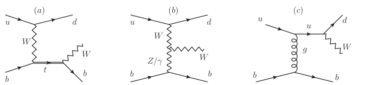
Figure 1: (a) resonant tree-level diagram contributing to $A^{(3,0)}_{(-1)}$ and $A^{(3,0)}_{(0)}$; (b) example of a background diagram contributing to $A^{(3,0)}_{(0)}$; (c) example of a QCD diagram contributing to $A^{(1,2)}$.

Within the ET framework, the leading contribution to ${\cal A}^{{\rm tree}}$ is reproduced in three steps: production of an on-shell top (through an operator in the ET with its matching coefficient), propagation of a resonant top (through the leading bilinear top operator) and decay of an on-shell top ( through a decay operator in the ET with its matching coefficient). The bilinear operator resums the (gauge-invariant) hard part of the self energy. The subleading terms give rise to 5-point operators. Again, the operators as well as their matching coefficients are separately gauge invariant.

We aim at computing the cross section up to ${\cal O}(\delta^{3/2})\sim{\cal O}(\alpha_{\rm s}\delta)$, which corresponds to including one-loop QCD corrections to the leading resonant part. Within the ET approach this will amount to computing one-loop corrections to the Wilson coefficients for the leading production and decay operators, as well as explicit calculation of one-loop corrections within the effective theory. To illustrate the connection between the ET and standard loop calculations, let us consider two examples, shown in Figure 2.

Figure 2: Two examples of how usual loop diagrams are reproduced by the ET. Grey lines indicate soft gluons, solid (hollow) dots indicate tree-level (one-loop) matching coefficients.

Example (a) illustrates how the self-energy is split into a hard part and a soft part. The hard part scales as ${\cal O}(\delta^{0})$ and, therefore, has to be resummed. The soft part is suppressed by an additional power $\delta^{1/2}$ with respect to ${\cal A}^{{\rm tree}}$. Thus we need to include only one soft self-energy insertion at ${\cal O}(\delta^{3/2})$. Example (b) illustrates how a normal loop diagram is split into a hard (factorizable) contribution included in the matching coefficient and a soft (non-factorizable) contribution where the gluon is still dynamical in the ET. The situation is not affected by including an arbitrary number of hard self-energy contributions to the top propagator, but an additional soft self-energy insertion results in a contribution beyond ${\cal O}(\delta^{3/2})$.

The ET allows us to identify and compute the minimal set of corrections needed at a certain order in $\delta$. In particular a full one-loop calculation including all non-resonant diagrams is not needed at this order. The price to be paid for this simplification is that we have to insist on the kinematical constraint $\Delta/m_{t}^{2}\ll 1$. A corresponding calculation using e.g. the complex mass scheme [9] would be more complicated, but would allow us to study observables without this constraint.

3 Real corrections

Using an ET approach as described in the previous section is a well established tool for the calculation of total cross sections [10]. When computing real corrections for more general observables within an ET approach we run into difficulties. The problem is related to the fact that an ET approach relies on knowing and making explicit all scales of the problem. As long as we have not precisely defined the observable we are interested in, this is not the case.

In Section 2 we based the expansion on the small scale $\Delta$ (and the couplings), implicitly assuming there are no further small scales. While this does put some restrictions on possible observables (similar to any fixed-order calculation) it allows us to study a large class of physical quantities. In the case of real corrections, we have an additional gluon present in the final state. Depending on $p_{7}$, the momentum of the gluon, the expansion parameter does change. Consider e.g. the case where $p_{7}$ is collinear to $p_{4}$, the momentum of the outgoing $b$ quark. In this case $p_{7}$ and $p_{4}$ will combine to a jet and the proper expansion parameter would be $(p_{4}+p_{7}+p_{W})^{2}-m_{t}^{2}$. On the other hand, if $p_{7}$ is well resolved, this will give rise to an additional (gluon) jet and the proper expansion parameter would be $(p_{4}+p_{W})^{2}-m_{t}^{2}$, as in Section 2.

In order to deal with this we deviate from a strict ET approach. Using the subtraction method to compute the real corrections we write

$$\int d\Phi_{n+1}M_{n+1} = \int d\Phi_{n+1}\left(M_{n+1}-M^{\rm sing}_{n(+1)}\right)+\int d\Phi_{n+1}\,M^{\rm sing}_{n(+1)}$$

$$\simeq \int d\Phi_{n+1}\left(M_{n+1}-M^{\rm sing}_{n(+1)}\right)+\int d\Phi_{n+1}\,M^{\rm sing\ {exp}}_{n(+1)}$$

Here $M_{n+1}$ is the matrix element squared for the process $u\,b\to d\,b\,e^{+}\,\nu\,g$ and $M^{\rm sing}_{n(+1)}$ denote the limits of the matrix elements in the singular (soft and collinear) regions. Upon phase-space integration the term $\int d\Phi_{n+1}M^{\rm sing}_{n(+1)}$ would match the infrared singularities of the full virtual one-loop amplitude. Since we use only the expanded virtual term, there is a mismatch between the singularities. Fortunately, the singular limits have only $n$-parton kinematics and we can use the same expansion as for the tree-level and virtual amplitudes. Computing $\int d\Phi_{n+1}\,M^{\rm sing\ {exp}}_{n(+1)}$, i.e. integrating the expanded singular limits over the phase space, produces the same infrared singularities as the expanded virtual corrections. In the first term on the r.h.s. of Eq. (3) we do not perform any expansion. The mismatch between what we subtract and what we add back is subleading in $\delta$ and beyond the accuracy we are aiming at.

In principle we should use the full matrix element $M_{n+1}$ in Eq. (3) to ensure gauge invariance. We can simplify the calculation by taking only resonant real diagrams. This potentially introduces a gauge dependence which, however, is beyond the accuracy of our calculation. Thus the situation is completely analogous to the renormalization or factorization scale dependence, which is widely accepted as long as it is beyond the accuracy of the calculation. A variation of $\mu$ within a reasonable window tells us as much (or as little) about the size of neglected higher-order terms as a variation of the gauge parameter $\xi$ within a window around 1. Of course, it is always possible that there are terms that are parametrically of higher order, but numerically important. This is usually associated with the presence of widely different scales and requires additional resummations.

4 Results and outlook

We are now ready to compute an arbitrary infrared-safe quantity at ${\cal O}(\delta^{3/2})$. As always, the word arbitrary has to be taken with some caution. First of all we have to enforce the constraint $\Delta\sim m_{t}\Gamma_{t}$. Second, we implicitly assume there are no other small scales introduced through the observable. A similar requirement is present for any fixed-order calculation.

As an example we consider $u\,b\to W$ plus jets, defining the jets using a $k_{\perp}$ cluster algorithm. We require a $b$ jet, $J_{b}$, and at least one more jet, both with $p_{\perp}>20$ GeV. In addition we require $150~{}{\rm GeV}\leq M^{\rm inv}\leq 200$ GeV, where $M^{\rm inv}=\sqrt{(p_{W}+p_{J_{b}})^{2}}$ is the invariant mass of the ($W\,J_{b}$) pair. We stress that we could add cuts on the decay products of the $W$ or any other ’reasonable’ cuts.

In Figure 3 we show the $M^{\rm inv}$ and $M^{T}$ distribution for the LHC with $\sqrt{s}=10$ GeV, where $M^{T}$ is the transverse mass of the ($W\,J_{b}$) system. We set $\mu_{F}=\mu_{R}=100$ GeV, $m_{t}=171.3$ GeV and $\Gamma_{t}=1.32$ GeV and use NLO MSTW pdfs [11] for the LO and NLO results. Compared to previous NLO calculations [12] our result also includes non-factorizable corrections which leads to a small but visible deviation from a Breit-Wigner shape in the in the $M^{\rm inv}$ distribution.

  

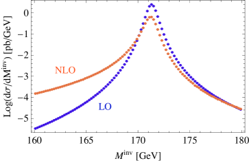
Figure 3: Invariant and transverse mass distribution at ${\cal O}(\delta)$ (blue, dark) and ${\cal O}(\delta^{3/2})$ (red, light).

Of course, the results shown in Figure 3 are not complete, since at NLO we also have to include gluon-initiated processes and there are other partonic initial states such as $b\,u\to d\,b\,W$ and $c\,b\to s\,b\,W$. A full analysis as well as the potential impact of non-factorizable corrections on a measurement of $m_{t}$ for single top and in particular $t\bar{t}$ pair production is left for future work.

References

-
[1]
R. G. Stuart,
Phys. Lett. B262, 113 (1991);
A. Aeppli, G. J. van Oldenborgh and D. Wyler, Nucl. Phys. B428, 126 (1994), [hep-ph/9312212]. - [2] V. S. Fadin, V. A. Khoze and A. D. Martin, Phys. Rev. D49, 2247 (1994).
-
[3]
K. Melnikov and O. I. Yakovlev,
Nucl. Phys. B 471 (1996) 90
[hep-ph/9501358];
W. Beenakker, A. P. Chapovsky and F. A. Berends, Nucl. Phys. B 508 (1997) 17 [hep-ph/9707326];
A. Denner, S. Dittmaier and M. Roth, Nucl. Phys. B 519 (1998) 39 [hep-ph/9710521];
N. Kauer, Phys. Rev. D 67 (2003) 054013 [arXiv:hep-ph/0212091]. -
[4]
R. Pittau,
Phys. Lett. B 386 (1996) 397 [arXiv:hep-ph/9603265];
W. Beenakker et al., Phys. Lett. B 454 (1999) 129 [arXiv:hep-ph/9902304]. -
[5]
V. S. Fadin, V. A. Khoze and A. D. Martin,
Phys. Rev. D 49 (1994) 2247;
K. Melnikov and O. I. Yakovlev, Phys. Lett. B 324 (1994) 217 [hep-ph/9302311]. - [6] A. P. Chapovsky et al., Nucl. Phys. B621, 257 (2002), [hep-ph/0108190].
-
[7]
M. Beneke and V. A. Smirnov,
Nucl. Phys. B522 (1998) 321 [hep-ph/9711391];
- [8] M. Beneke et al., Nucl. Phys. B 686 (2004) 205 [arXiv:hep-ph/0401002].
- [9] A. Denner and S. Dittmaier, Nucl. Phys. Proc. Suppl. 160 (2006) 22 [arXiv:hep-ph/0605312].
-
[10]
A. H. Hoang et al.,
Eur. Phys. J. direct C 2 (2000) 1
[arXiv:hep-ph/0001286];
M. Beneke et al., Nucl. Phys. B 792 (2008) 89 [arXiv:0707.0773 [hep-ph]]. - [11] A. D. Martin et al., Eur. Phys. J. C 63 (2009) 189 [arXiv:0901.0002 [hep-ph]].
- [12] J. M. Campbell et al., Phys. Rev. Lett. 102 (2009) 182003 [arXiv:0903.0005 [hep-ph]].