Quantum Algorithm of Evolutionary Analysis of 1D Cellular Automata

Abstract

It is shown that irreversible classical cellular automata can be performed by quantum algorithm using additional ancilla registers. The algorithm for cellular automata states analysis has been proposed. This algorithm is based on the elements of Grover’s algorithm - the inversion of amplitude of searched states and unitary transform of inversion about the average. The inversion of searched states amplitudes can be performed by quantum Toffoli gate.

Introduction

The cellular automata (CA) is a computational model which has been studied in many scientific works . These models are based on simple updating rules and show the perspective for computational applications.

The aim of our study is to design the algorithms which allow to use quantum parallelism for the investigation of CA evolution for all initial states simultaneously. For example, if one dimensional CA consists from only 100 cells with 2 possible states, then one quantum evolution can evaluate $2^{100}$ evolutions for the same number of initial states. It is important to answer a question - does or does not some searched finish state (”good state”) in CA evolution for analyzed CA updating rules exist? We will use Grover’s algorithms ideas to answer this question in case of one dimensional quantum cellular automata.

Quantum cellular automata (QCA) are being investigated in many modern works. In the work [2] QCA for universal quantum computation has been presented. In [3, 4] one dimensional QCA has been investigated. In [5] QCA formalism based on a lattice of qubits has been described. In [6, 7] reversible QCA was considered. In [8, 9] the survey of QCA investigations has been presented.

One Dimension Cellular Automata

Let us consider the ability of implementation of synchronous cellular automata by the quantum logical gates when all cells switch to a new state simultaneously. Such a circuit can be performed by using additinal qubits named ancilla. Let us consider for determinance one of CA rules for updating CA states. For example, a cell switches to state ”0” if its neighbors have the same value, otherwise this cell switches to value ”1”. This rule can be written as

$$x^{{}^{\prime}}[i]:=x[i-1]\oplus x[i+1].$$ (1)

In the classical CA such evolution is irreversible. If the results of previous iteration are saved in an additional ancilla, then CA evolution reversibility and unitarity can be achieved. Consider unitary operator for performing rule (1). This operator acts on three qubits - $|x_{i-1}\rangle,|x_{i+1}\rangle$ , $|a_{i}\rangle$ two neighbors and ancilla from the additional register:

$$C=(X\otimes X\otimes I)\cdot T\cdot(X\otimes X\otimes I)\cdot T\cdot(I\otimes I\otimes X).$$ (2)

Before the iteration all additional ancilla are in the state

$$|0,0,\ldots,0\rangle_{n}$$ (3)

The series of unitary transformations for qubits can be written as

$$C_{i}:I\otimes I\otimes X|x_{i-1},x_{i+1},0\rangle\rightarrow T|x_{i-1},x_{i+1},1\rangle\rightarrow|x_{i-1},x_{i+1},1\oplus x_{i-1}x_{i+1}\rangle$$

$$\rightarrow X\otimes X\otimes I|x_{i-1},x_{i+1},1\oplus x_{i-1}x_{i+1}\rangle\rightarrow|\neg x_{i-1},\neg x_{i+1},1\oplus x_{i-1}x_{i+1}\rangle$$

$$\rightarrow T|\neg x_{i-1},\neg x_{i+1},1\oplus x_{i-1}x_{i+1}\rangle\rightarrow|\neg x_{i-1},\neg x_{i+1},1\oplus x_{i-1}x_{i+1}\oplus\neg x_{i-1}\neg x_{i+1}\rangle$$

$$\rightarrow X\otimes X\otimes I|\neg x_{i-1},\neg x_{i+1},1\oplus x_{i-1}x_{i+1}\oplus\neg x_{i-1}\neg x_{i+1}\rangle\rightarrow|x_{i-1},x_{i+1},x_{i}^{t+1}\rangle$$ (4)

The action of operator $C_{i}$ on the possible qubits values can be described as

$$C_{i}:|0\rangle_{i-1,t}|0\rangle_{i+1,t}|0\rangle_{a,t+1}\rightarrow|0\rangle_{i-1,t}|0\rangle_{i+1,t}|0\rangle_{a,t+1}$$

$$C_{i}:|1\rangle_{i-1,t}|1\rangle_{i+1,t}|0\rangle_{a,t+1}\rightarrow|1\rangle_{i-1,t}|1\rangle_{i+1,t}|0\rangle_{a,t+1}$$

$$C_{i}:|1\rangle_{i-1,t}|0\rangle_{i+1,t}|0\rangle_{a,t+1}\rightarrow|1\rangle_{i-1,t}|0\rangle_{i+1,t}|1\rangle_{a,t+1}$$

$$C_{i}:|0\rangle_{i-1,t}|1\rangle_{i+1,t}|0\rangle_{a,t+1}\rightarrow|0\rangle_{i-1,t}|1\rangle_{i+1,t}|1\rangle_{a,t+1}$$ (5)

CA updating rules (1)-(5) can be described by quantum circuit in fig.1

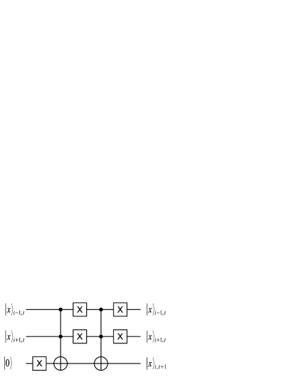
Figure 1: Quantum circuit implementation for CA updating rules

CA state at $j$ iteration can be described using the following operator

$$A_{j}=C_{n}\ldots C_{2}C_{1}.$$ (6)

Let us consider the first CA iteration with the additional ancilla register.

$$A_{1}:|x\rangle_{0}|0\rangle_{1}\rightarrow|x\rangle_{0}|f(x)\rangle_{1}.$$ (7)

where $|x\rangle=|x_{1},x_{2}\ldots x_{n}\rangle$ - is initial CA register, $f(x)$ - is some function which expresses CA rules for CA updating (1)-(5). On the next iteration the new ancilla register is being added. It can be described as

$$A_{2}:|x\rangle_{0}|f(x)\rangle_{1}|0\rangle_{2}^{\otimes n}\rightarrow|x\rangle_{0}|f(x)\rangle_{1}|f(f(x))\rangle_{2}.$$ (8)

CA evolution after $m$ iteration can be written as

$$A_{m}\ldots A_{2}A_{1}:|x\rangle_{0}|0\rangle_{1}^{\otimes n}\ldots|0\rangle_{m}^{\otimes n}\rightarrow|x\rangle_{0}|f(x)\rangle_{1}\ldots|f^{(m)}(x)\rangle_{m}.$$ (9)

Our next step is to perform the iteration which is inversed to the one that is defined by operator $A_{m-1}$, where

$$A_{m-1}(A_{m-1})^{-1}=I.$$ (10)

Applying of such an operator to the registers system after $m$ iterations (9) can be written as

$$(A_{m-1})^{-1}:|x\rangle_{0}|f(x)\rangle_{1}\ldots|f^{(m-1)}(x)\rangle_{m-1}|f^{(m)}(x)\rangle_{m}\rightarrow$$

$$\rightarrow|x\rangle_{0}|f(x)\rangle_{1}\ldots|0\rangle_{m-1}^{\otimes n}|f^{(m)}(x)\rangle_{m}.$$ (11)

A set of inversed transformations can be written as

$$(A_{1})^{-1}\ldots(A_{m-2})^{-1}(A_{m-1})^{-1}:|x\rangle_{0}|f(x)\rangle_{1}\ldots|f^{(m-1)}(x)\rangle_{m-1}|f^{(m)}(x)\rangle_{m}\rightarrow$$

$$\rightarrow|x\rangle_{0}|0\rangle_{1}^{\otimes n}\ldots|0\rangle_{m-1}^{\otimes n}|f^{(m)}(x)\rangle_{m}.$$ (12)

As a result of applying the operators of inversed evolutions, the registers of additional qubits will be in initial states and can be removed without the affection on other qubits. General evolution of CA can be described by operator

$$U_{CA}=(A_{1})^{-1}\ldots(A_{m-2})^{-1}(A_{m-1})^{-1}A_{m}A_{m-1}\ldots A_{1}.$$ (13)

The resulted evolution of quantum CA can be written as

$$U_{CA}:|x\rangle|0\rangle^{\otimes n}\rightarrow|x\rangle|f^{(m)}(x)\rangle.$$ (14)

Let us consider the steps of implementation of quantum cellular automata:

1. At the first step the CA register in the basic state is initialized

   $$|x_{1},x_{2},\ldots x_{n}\rangle_{n}\rightarrow|0_{1},0_{2},\ldots 0_{n}\rangle_{n}$$ (15)

2. Let us apply the Hadamar operator to each qubit of CA register. This operator is given by matrix

   $$H=\frac{1}{\sqrt{2}}\left(\begin{array}[]{cc}1&1\\ 1&-1\\ \end{array}\right).$$ (16)

3. As a result we obtain the following superposition

   $$H^{\otimes n}|0_{1},0_{2},\ldots 0_{n}\rangle_{n}=\frac{1}{\sqrt{2^{n}}}\sum_{x=1}^{x=2^{n}}{|x\rangle}$$ (17)

   where $|x\rangle$ denotes computational basis states $|x_{1},x_{2},\ldots x_{n}\rangle_{n}$

   The Hadamar transformation generates the superposition of all possible $2^{n}$ states with the equal amplitudes.

   Let us apply unitary transformation (14)

   $$|\Psi_{CA}\rangle=U_{CA}\left(H^{\otimes n}|0\rangle^{\otimes n}\right)|0\rangle^{\otimes n}=\frac{1}{\sqrt{2^{n}}}\sum_{x=1}^{2^{n}}{|x\rangle|f^{(m)}(x)}\rangle$$ (18)

   Superposition $|\Psi_{CA}\rangle$ includes all $2^{n}$ results of evolutions initial states of CA with dimension n. With one quantum evolution of CA, all possible CA evolutions for initial states with defined CA updating rules are performed.

Analysis of Cellular Automata Evolution

Let us consider the ability to amplify the amplitudes of searched states with using the ideas of Grover’s algorithm which is being being used for searching files in the quantum database [10, 11, 12]. The difference between this task and Grover’s algorithm is that unknown states are not being searched in this task, these searched states are known and we need to get the answer that such states exist in CA evolution. Let us introduce an additional qubit - ancilla which will be controlled by n-qubit Toffoli gate where n-qubit of CA state are controlling the ancilla state in the Toffoli gate. This gate can be described by unitary matrix

$$T=\left(\begin{array}[]{cccc}1&\ldots&\ldots&0\\ \ldots&\ldots&\ldots&\ldots\\ \ldots&\ldots&0&1\\ 0&\ldots&1&0\\ \end{array}\right).$$ (19)

Let us consider the unitary operator which is defined as tensor product of one qubits operators

$$S_{T}=\bigotimes_{i=1}^{n}S_{i}$$ (20)

where

$$S_{i}=\left\{\begin{array}[]{ll}I,&\textrm{ $e_{i}=1$}\\ X,&\textrm{ $e_{i}=0$}\end{array}\right.$$ (21)

The operator $S_{T}$ flips searched states $|e_{1},e_{2},\ldots e_{n}\rangle$ into the state $|1_{1},1_{2},\ldots 1_{n}\rangle$. It is necessary for implementation of anclilla inversion for searched states by Toffoli transformation (19) Apply hadamar operator to ancilla $|z\rangle$ in prepared state $|1\rangle$

$$|z\rangle=H|1\rangle=\frac{1}{\sqrt{2}}(|0\rangle-|1\rangle)$$ (22)

Let consider an operator

$$U_{T}=(I^{\otimes n}\otimes S_{T}\otimes I)(I^{\otimes n}\otimes T_{n})(I^{\otimes n}\otimes S_{T}\otimes I)$$ (23)

Let apply this operator to the system of qubits registers $|x\rangle|f^{(m)}(x)\rangle|z\rangle$. the first group of operators on the right side which is delimited by brackets performs flipping into the state $|1_{1},1_{2},\ldots 1_{n}\rangle$ of searched finish states, the second group performs ancilla $|z\rangle$ inversion for searched states and the third group returns states which are changed by the first group into the state before applying the operator. Additional controlled qubit stays in the state (22). The result of the operator (23) acting is

$$U_{T}(|x\rangle|f^{(m)}(x)\rangle|z\rangle)=\frac{1}{\sqrt{2^{n}}}\left(\sum_{x\notin X_{q}}|x\rangle|f^{(m)}(x)\rangle-\sum_{x\in X_{q}}|x\rangle|q\rangle\right)\otimes|z\rangle$$ (24)

where $X_{q}$ - is set of initial states $|x\rangle$, which leads to the searched states $|q\rangle$ in the CA evolutional process after $m$ CA iterations. Ancilla $|z\rangle$ in a new basis leaves in the unchanged state, but in the superpositions states the inversion of amplitudes signs for subsystem $\sum_{x\in X_{q}}|x\rangle|q\rangle$ appears. It is caused by the transformation of ancilla $|z\rangle$ to new state (22) before applying the operator (24).

Let us consider the inversion operator from Grover’s algorithm

$$U_{G}=2|\Psi_{c}\rangle\langle\Psi_{c}|-I$$ (25)

where

$$|\Psi_{c}\rangle=H^{\otimes n}|0\rangle^{\otimes n}=\frac{1}{\sqrt{2^{n}}}\sum_{i=1}^{i=2^{n}}{|i\rangle}$$ (26)

This operator will be used for the states $\sum_{x\in X_{q}}|x\rangle|q\rangle$ amplitudes amplification. The operator $U_{G}$ reflect any vector around the axis defined by vector $|\Psi_{c}\rangle$. The operator $U_{G}$ can be decomposed by one-qubit operators

$$U_{G}=H^{\otimes n}(2|0\rangle\langle 0|-I)H^{\otimes n}$$ (27)

The operator $U_{G}$ also has been called as the operator of inversion about the average. The transformation (25) can also be defined as

$$U_{G}:\sum_{i}{a_{i}|i\rangle}\rightarrow\sum_{i}{(2A-a_{i})|i\rangle}$$ (28)

where $A$ - means the average value of $a_{i}$ amplitudes.

If searched state $\sum_{x\in X_{q}}|x\rangle|q\rangle$ can be realized only once from one initial CA state, then its amplitude is

$$\beta=\frac{1}{\sqrt{2^{n}}}$$ (29)

It can be shown that performing of CA iteration

$$U_{G}U_{T}(|x\rangle|f^{(m)}(x)\rangle|z\rangle)$$ (30)

we obtain the amplitude amplification by 3 times that match the implementation of inversion iteration in the Grover’s algorithm [10, 11, 12]. The transformation $U_{G}U_{T}$ can be described by quantum circuit in fig.2.

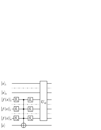
Figure 2: Quantum circuit implementation of the transformation $U_{G}U_{T}$

Let us consider the number of iterations necessary for enough amplification of searched states amplitudes. If only one initial state $|x\rangle$ of cellular automata leads to the searched finish state $|q\rangle$, then using the ideas similar to Grover’s algorithms [10, 11, 12] we can find the optimal number of unitary transform $U_{G}U_{T}$ .

$$k\approx\frac{\pi}{4}\sqrt{N},N=2^{n}$$ (31)

It follows from this result that algorithm complexity is $O(\sqrt{N})$. In comparision with analogical classical algorithm $O(N)$ it means polinomial computational speedup. If instead 1 matching initial state there are $l$ matching states which lead to the searched finish state, then

$$k\approx\frac{\pi}{4}\sqrt{\frac{N}{l}},$$ (32)

if $l$ is unknown, then Grover’s algorithm could be run several times when

$$L=1,2,4,8\ldots$$ (33)

It can be shown, that for such series calculation the complexity will be still $O(\sqrt{N})$.

Conclusion

It is shown that irreversible classical cellular automata can be performed by quantum algorithm using additional ancilla registers. The algorithm for cellular automata states analysis has been proposed. This algorithm is based on the elements of Grover’s algorithm - the inversion of amplitude of searched states and unitary transform of inversion about the average. The inversion of searched states amplitudes can be performed by quantum Toffoli gate.

References

• [1] S. Wolfram, Universality and complexity in cellular automata, Physica D, 10, (1984), p.1-35.
• [2] K.G.H. Vollbrecht, J.I. Cirac, Reversible universal quantum computation within translation-invariant systems, Phys. Rev. A 73, 012324 (2006)
• [3] Pablo Arrighi, Renan Fargetton, and Zizhu Wang, Intrinsically universal one-dimensional quantum cellular automata in two avours, arXiv:0704.3961v3 (2008)
• [4] Pablo Arrighi, Vincent Nesme, Reinhard Werner, One-dimensional quantum cellular automata over finite, unbounded configurations, arXiv:0711.3517v1 (2007)
• [5] Carlos A. Perez-Delgado, Donny Cheung Local Unitary Quantum Cellular Automata, arXiv:0709.0006v1 (2007)
• [6] B. Schumacher, R.F. Werner, Reversible Quantum Cellular Automata, arXiv:quant-ph/0405174v1, (2004)
• [7] Dirk-M. Schlingemann, Holger Vogts, Reinhard F. Werner, On the structure of Clifford quantum cellular automata, arXiv:0804.4447v1 (2008)
• [8] Karoline Wiesner, Quantum Cellular Automata, arXiv:0808.0679v1 (2008)
• [9] B. Aoun, M. Tarifi, Introduction to Quantum Cellular Automata, arXiv:quant-ph/0401123v1 (2004)
• [10] L.K. Grover, Quantum Mechanics helps in searching for a needle in haystack, Phys.Rev. Lett. 79(2):325-328, 1997,
• [11] C. Zalka, Grover’s quantum searching algorithm is optimal, Phys. Rev. A., 60(4):2746-2751, 1999.
• [12] C. Lavor, L.R.U. Manssur, R. Portugal, Grover’s Algorithm: Quantum Database Search, arXiv:quant-ph/0301079v1 (2003)