Entropy and specific heat for open systems in steady states

Abstract

The fundamental assumption of statistical mechanics is that the system is equally likely in any of the accessible microstates. Based on this assumption, the Boltzmann distribution is derived and the full theory of statistical thermodynamics can be built. In this paper, we show that the Boltzmann distribution in general can not describe the steady state of open system. Based on the effective Hamiltonian approach, we calculate the specific heat, the free energy and the entropy for an open system in steady states. Examples are illustrated and discussed.

I introduction

The fundamental postulate in statistical mechanics is as follows: For a conservative system the path of the system in phase space passes through all points of the energy surface and in such a manner that this surface is covered uniformly. This postulate (called ergodic hypothesis) indicates that a conservative system in equilibrium does not have any preference for any of its available microstates, i.e., given $\Omega$ microstates at a particular energy, the probability of finding the system in a particular microstate is $p=1/\Omega$. By using the ergodic hypothesis, one can conclude that for a system at equilibrium, the thermodynamic state which results from the largest number of microstates is the most probable macrostate of the system. With these results, the probability $p_{i}$ that a macroscopic system in thermal equilibrium with its environment in a given microstate with energy $E_{i}$ can be derived, $p_{i}=exp(-\beta E_{i})/\sum_{j}exp(-\beta E_{j})$ and $\beta=1/k_{B}T,$ which is the so-called Boltzmann distribution.

It is believed that a generic system that interacts with a generic environment evolves into an equilibrium described by the Boltzmann distributiondevi09 . Experience shows that this is true but a detailed understanding of this process, which is crucial for a rigorous justification of statistical physics and thermodynamics, is lackingreimann08 ; goldstein06 ; popescu06 ; tasaki98 ; jensen85 ; bocchieri59 . The key question is to what extent the evolution to equilibrium depends on the details of the system-environment couplingbertin09 . In fact, detailed analysis shows that it is not always the case that the system evolves into the equilibrium state described by Boltzmann distribution. Then two questions arise: (1) Given a dynamical process, how far does the steady state differ from the equilibrium state? (2)What is the free energy and specific heat of such a system?

Here, we shall answer these questions by considering an open system coupled to two independent environments at different temperatures. The dynamics of the open system is assume to fulfill a master equation in the Lindblad form, steady state is achieved by the effective Hamiltonian approach. We find that the steady state is not the thermal equilibrium state even if the environments have the same temperature. Free energy, the specific heat and the entropy are calculated and discussed.

II formalism

Imagine to prepare an open quantum system surrounded by two independent environments at different temperatures $T_{1}$ and $T_{2}$, respectively. See Fig.1.

Figure 1: (Color online) A given system immersed in two environments at temperature $T_{1}$ and $T_{2}$, respectively. Eventually, the system arrives at a steady state depending on the system-environment couplings and the temperature.

In the weak coupling limit and under the Markov approximation, the dynamics of the quantum system is govern by,

$$i\frac{\partial}{\partial t}\rho = [H,~{}\rho]+\mathcal{L}_{1}\rho+\mathcal{L}_{2}\rho,$$ (1)

where $\mathcal{L}_{1}\rho=\frac{i}{2}\sum_{k}\gamma_{k}(T_{1})(2L_{k}\rho L_{k}^{{\dagger}}-L_{k}^{{\dagger}}L_{k}\rho-\rho L_{k}^{{\dagger}}L_{k}),\mathcal{L}_{2}\rho=\frac{i}{2}\sum_{k}\Gamma_{k}(T_{2})(2X_{k}\rho X_{k}^{{\dagger}}-X_{k}^{{\dagger}}X_{k}\rho-\rho X_{k}^{{\dagger}}X_{k}).$ $\rho(t)$ represents the reduced density matrix of the system, $H$ represents the free Hamiltonian of the system and $L_{k}(L_{k}^{\dagger})$ and $X_{k}(X_{k}^{\dagger})$ are operators of the system through which the system and its environments coupled. The master equation can be solved by the effective Hamiltonian approachyi01 .

The main idea of The effective Hamiltonian approach can be outlined as follows. By introducing an ancilla, which has the same dimension of Hilbert space as the system, we can map the system density matrix $\rho(t)$ to a wave function of the composite system (system + ancilla). A Schrödinger -like equation can be derived from the master equation. The solution of the master equation can be obtained by mapping the solution of the Schrödinger -like equation back to the density matrix. Assume the dimension of the Hilbert space for both the system and the ancilla is $N$, and let $|E_{n}(0)\rangle$ and $|e_{m}(0)\rangle$ denote the eigenstates for the system and the ancilla, respectively. The mathematical representation of the above idea can be formulated as follows. A wave function for the composite system in the $N^{2}$-dimensional Hilbert space may be constructed as $\rho(t)\rightarrow|\Psi(t)\rangle_{\rho}=\sum_{m,n=1}^{N}\rho_{mn}(t)|E_{m}(0)\rangle|e_{n}(0)\rangle,$ where $\rho_{mn}(t)=\langle E_{m}(0)|\rho(t)|E_{n}(0)\rangle$. Note that ${}_{\rho}\langle\Psi|\Psi\rangle_{\rho}=\text{Tr}(\rho^{2})\leq 1$, i.e. this pure bipartite state is not normalized except when the state of the open system is pure. With these definitions, the master equation ($\hbar=1$ hereafter) can be rewritten in a Schrödinger-like equationyi01

$$i\frac{\partial}{\partial t}|\Psi(t)\rangle_{\rho}=\mathcal{H}_{\text{eff}}|\Psi(t)\rangle_{\rho},$$ (2)

where $\mathcal{H}_{\text{eff}}$ is the so-called effective Hamiltonian and is defined by

$$\mathcal{H}_{\text{eff}}=\mathcal{H}-\mathcal{H}^{A}$$

$$+i\sum_{k}\gamma_{k}(T_{1})L_{k}^{A}L_{k}+i\sum_{k}\Gamma_{k}(T_{2})X_{k}^{A}X_{k},$$ (3)

where $\mathcal{H}=H-\frac{i}{2}\sum_{k}\gamma_{k}(T_{1})L_{k}^{{\dagger}}L_{k}-\frac{i}{2}\sum_{k}\Gamma_{k}(T_{2})X_{k}^{{\dagger}}X_{k},$ $\mathcal{H}^{A}$, $L^{A}_{k}$ and $X^{A}_{k}$ are operators for the ancilla defined by ($O=L,X,H$), $\langle e_{m}(0)|O^{A}|e_{n}(0)\rangle=\langle E_{n}(0)|O^{{\dagger}}|E_{m}(0)\rangle.$ By this effective Hamiltonian approach, it is easy to prove that the steady state $\rho_{S}$ can be given by mapping the eigenstate of $\mathcal{H}_{\text{eff}}$ with zero eigenvalue. Namely, calculating $|R_{0}\rangle$ by

$$\mathcal{H}_{\text{eff}}|R_{0}\rangle=0,$$ (4)

we can obtain elements of the steady state density matrix, $\rho_{S,mn}=\langle E_{m}(0)|\rho_{S}|E_{n}(0)\rangle=\langle E_{m}(0)|\langle e_{n}(0)|R_{0}\rangle.$ Given a steady state, the single-particle energy $U$ would be equal to,

$$U=\text{Tr}(\rho_{S}H).$$ (5)

If a system consists of many non-interacting particles, the total energy equals to the sum of the single-particle energy. The specific heat for a single particle now would be given by

$$C_{T_{i}}=\frac{\partial U}{\partial T_{i}}.$$ (6)

Given the steady state density matrix $\rho_{S}$, von Neumann defined the entropy as

$$S=-\rho_{S}\ln\rho_{S},$$ (7)

which is a proper extension of the Gibbs entropy to the quantum case. We note that the entropy $S$ times the Boltzmann constant $k_{B}$ ($k_{B}=1$ in this Letter) equals the thermodynamical entropy. If the system is finite dimensional, the entropy describes the distance of the steady state from a pure state.

III examples

To illustrate the general formalism, we present here three examples. In the first example, we consider a two-level system coupled to two independent environments at different temperatures $T_{1}$ and $T_{2}$, respectively. The dynamics is described by Eq.(1) with $\gamma_{1}(T_{1})=\gamma\bar{n}_{1},~{}~{}\gamma_{2}(T_{1})=\gamma(\bar{n}_{1}+1),$ $L_{1}=\sigma^{+},~{}~{}L_{2}=\sigma^{-},$ $\Gamma_{1}(T_{2})=\Gamma(2\bar{n}_{2}+1),~{}~{}X_{1}=\sigma^{x}$ and $\bar{n}_{i}=\frac{1}{e^{\beta_{i}\Omega}-1}(i=1,2).$ The system Hamiltonian is specified to be $H=\frac{\Omega}{2}\sigma^{z}.$ By the effective Hamiltonian approach, we arrive at density matrix elements of the steady state $\frac{\rho_{11}}{\rho_{00}}=\frac{\gamma_{1}+\Gamma_{1}}{\gamma_{2}+\Gamma_{1}}$ with the trace preserving condition $\rho_{11}+\rho_{00}=1.$ Fig.2 depicts the specific heat $C_{T_{1}},C_{T_{2}}$, the free energy $U$ and the entropy $S$ as a function of temperature $T_{1}$ and $T_{2}$. We note that for $T_{1}\rightarrow 0$ and $T_{1}\rightarrow\infty$ the specific heat $C_{T_{1}}$ tends to zero, the population is then said to be frozen. For a fixed $T_{1}$ being of order of $\Omega$, $C_{T_{1}}$ decreases as $T_{2}$ increases, and $C_{T_{1}}$ tends to zero as $T_{2}\rightarrow\infty$. $C_{T_{2}}$ behaves similarly. The free energy $U$ and the entropy $S$ approach constants with $T_{1}$ and $T_{2}$ tend to infinity, confirming that the population is frozen at sufficiently high temperatures. At low temperature, $U$ and $S$ increase as the temperature increases, indicating that the degree of mixture of the steady state grows with the increasing of temperature.

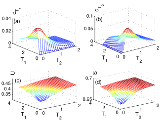
Figure 2: (Color online)The specific heat, the free energy and the entropy for the open two-level system as a function of temperature (in units of $\frac{\hbar\Omega}{k_{B}}$). The parameters chosen are $\gamma=0.2\Omega,$ $\Gamma=0.3\Omega.$ The energy was plotted in units of $\hbar\Omega$. The units for the specific heat and entropy were set accordingly.

We take two coupled qubits subject to decoherence as the second example. The system Hamiltonian is, $H=\Omega_{1}|e\rangle_{1}\langle e|+\Omega_{2}|e\rangle_{2}\langle e|+J\sigma^{x}_{1}\sigma^{x}_{2}.$ Suppose that the qubit 1 interacts with its environment at temperature $T_{1}$ via $\sigma_{1}^{-}$ and $\sigma_{1}^{+}$, while the qubit 2 through $\sigma_{2}^{x}$ couples to its environment at temperature $T_{2}$. The Liouvillian superoperators are then,

$$\mathcal{L}_{1}\rho=\frac{i}{2}\gamma(\bar{n}_{1}+1)(2\sigma^{-}_{1}\rho\sigma^{+}_{1}-\rho\sigma^{+}_{1}\sigma^{-}_{1}-\sigma^{+}_{1}\sigma^{-}_{1}\rho)$$

$$+\frac{i}{2}\gamma\bar{n}_{1}(2\sigma^{+}_{1}\rho\sigma^{-}_{1}-\rho\sigma^{-}_{1}\sigma^{+}_{1}-\sigma^{-}_{1}\sigma^{+}_{1}\rho)$$ (8)

and

$$\mathcal{L}_{2}\rho=\frac{i}{2}\Gamma(2\bar{n}_{2}+1)(2\sigma^{x}_{2}\rho\sigma^{x}_{2}-2\rho),$$ (9)

where $\bar{n}_{1}=\frac{1}{e^{\beta_{1}\Omega_{1}}-1},~{}~{}\bar{n}_{2}=\frac{1}{e^{\beta_{2}\Omega_{2}}-1}.$ $C_{T_{2}}\rightarrow 0$ as $T_{1}$ and $T_{2}$ tend to $\infty$ as Fig.3(b) shows. For $C_{T_{1}}$, however, it approaches a constant as $T_{2}\rightarrow\infty$ when $T_{1}$ takes a value of order of $\Omega_{i}$ (Fig.3(a)).

Figure 3: (Color online) The specific heats $C_{T_{1}}$ and $C_{T_{2}}$ versus temperature $T_{1}$ and $T_{2}$ for two interacting qubits dissipatively coupled to two independent environments. $\Omega_{1}=\Omega_{2},\gamma=0.2\Omega_{1},J=0.2\Omega_{1},\Gamma=0.3\Omega_{1}$ are chosen for this plot.

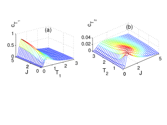
Figure 4: (Color online) $C_{T_{1}}$ and $C_{T_{2}}$ as a function of temperature and the coupling constant $J$. $T_{2}=1.5$ for (a) and $T_{1}=1.5$ for (b). The other parameters are the same as in Fig.3.

At $T_{1}=0,$ $C_{T_{1}}$ is always zero. For fixed $T_{1}$, $C_{T_{1}}$ tends to a constant with $J\rightarrow\infty,$ while $C_{T_{2}}$ always tends to zero as $J\rightarrow\infty,$ as Fig.4 shows. Equilibrium statistical mechanics tells us that the population of excited states (given by the Boltzmann distribution) grows as the temperature increases. The populations obtained from the steady state are different (see Fig.5). E. g., the population of the ground state increases as the temperature $T_{2}$ increases (Fig.5 (left)), whereas the population of the second excited state (labeled by (3)) decreases as the temperature increases. Similar observation can be found from Fig.5(right), the population of the first excited state decreases as the temperature $T_{1}$ increases. We will quantify this difference between the steady state and the equilibrium state by fidelity later.

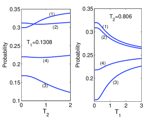
Figure 5: Probability for finding the system in the eigenstates of the Hamiltonian. $\Omega_{1}=\Omega_{2},\gamma=0.2\Omega_{1},J=0.2\Omega_{1},\Gamma=0.3\Omega_{1}.$ (1)-(4) label the eigenstates by the corresponding eigenvalues in increasing order, i.e., (1) labels the lowest eigenstate, while (4) the highest eigenstate.

In the third example, we consider a damped harmonic oscillator. The system Hamiltonian takes $H=\omega a^{{\dagger}}a.$ Consider a simple system-bath (at temperature $T_{1}$) Hamiltonian of the form $H_{int}=\sum_{j}g_{j}(b_{j}a^{\dagger}+b_{j}^{\dagger}a).$ The damping rates follows by the standard procedure, $\gamma_{1}(T_{1})=\gamma\bar{n}_{1},~{}~{}L_{1}=a^{{\dagger}}$, $\gamma_{2}(T_{1})=\gamma(\bar{n}_{1}+1),~{}~{}L_{2}=a.$ Suppose that the harmonic oscillator interacts with the environment at temperature $T_{2}$ through $(a^{{\dagger}}+a)$, the corresponding damping rate is $\Gamma_{1}(T_{2})=\Gamma(2\bar{n}_{2}+1),$ and $X_{1}=(a^{{\dagger}}+a).$ All these together give a master equation for the damped harmonic oscillator,

$$i\frac{\partial}{\partial t}\rho = [H,~{}\rho]+\frac{i}{2}\gamma_{1}(2a^{{\dagger}}\rho a-\rho aa^{{\dagger}}-aa^{{\dagger}}\rho)$$

$$+\frac{i}{2}\gamma_{2}(2a\rho a^{{\dagger}}-\rho a^{{\dagger}}a-a^{{\dagger}}a\rho)$$

$$+\frac{i}{2}\Gamma_{1}[2(a^{{\dagger}}{+}a)\rho(a^{{\dagger}}{+}a){-}(a^{{\dagger}}{+}a)^{2}\rho{-}\rho(a^{{\dagger}}{+}a)^{2}].$$

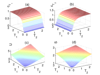
Figure 6: (Color online) Illustration of $C_{T_{1}},C_{T_{2}},U$ and $S$ as a function of temperature $T_{1}$ and $T_{2}$. In this plot, the dimension cutoff is $N=100,$ and $\gamma=0.3\omega,\Gamma=0.2\omega$. The energy is in units of $\hbar\omega$ and the temperature is in units of $\frac{\hbar\omega}{k_{B}}.$

Fig.6 shows the specific heat, the free energy, and the entropy as a function of temperature. We note that the specific heat $C_{T_{1}}$ ($C_{T_{2}}$) is vanishingly small for $T_{1}\rightarrow 0(T_{2}\rightarrow 0),$ it rises rapidly when $T_{1}$ ($T_{2}$) is of order of $\omega$ and approaches a limiting value, which depends on the damping rates $\Gamma_{1}$ and $\gamma.$ Note that at sufficiently high temperature, $C_{T_{i}}$ ($i=1,2$) are the same as that in equilibrium statistical mechanics.

The results presented in the examples clearly show that $C_{T_{i}}(i=1,2)$, $U$ and $S$ behaves different from those given by equilibrium statistical mechanics. The differences result from the deviation of the steady state density matrix from the equilibrium thermal state (Boltzmann distribution). We will use the fidelity to quantify this deviation. Fidelity as a measure of distance between two states is an important concept in quantum information theorynielsen00 . The well-known quantum fidelity for two general mixed states $\rho_{1}$ and $\rho_{2}$ is given by the Uhlmann’s fidelitybures69

$$F(\rho_{1},\rho_{2})=\mbox{Tr}\sqrt{\sqrt{\rho_{1}}\rho_{2}\sqrt{\rho_{1}}},$$ (11)

this fidelity possesses many advantages such as concavity and multiplicativity under tensor product and it satisfies all Josza’s four axiomsjozsa94 .

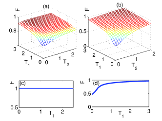
Figure 7: (Color online) Distance between the steady states and thermal states (Boltzmann distribution) measured by the fidelity as a function of temperature. (a) and (c) are for the damped oscillator, while (b) and (d) for the two coupled qubits. The steady state in (a) and (b) are obtained by solving the master equations Eqs. (8), (9) and (III). The steady states in (c) and (d) are for $\Gamma_{1}=0$ and $\Gamma=0,$ respectively. $\Omega_{1}=\Omega_{2},J=0.2\Omega_{1}.$

Fig.7 shows the fidelity between thermal states and the steady states. For both the coupled qubits and the damped harmonic oscillator, the fidelity arrives at its maximum when the temperatures tend to infinity (see Fig.7(a) and (b)). Note that the steady states depends on how the system couples to its environments. For example, the master equation Eq.(III) with $\Gamma_{1}=0$ can describe the thermalization of the oscillator, the simulation shows that this is exactly the case (Fig.7(c)). Differently, for the coupled two qubits system, the steady state given by the master equation (Eqs.(8) and (9)) with $\Gamma=0$ is not the equilibrium thermal state at low temperature (see Fig.7 (d)).

One may have doubts about the realizability of the master equations Eqs. (1), (8), (9) and (III). The technology in engineered reservoirsmyatt00 ; cirone09 shows that there is no problem to simulate an reservoir in which the system-environment coupling and state of the environment are controllable.

In summary, we study the deviation of steady state from equilibrium thermal state for an open system. The specific heat, free energy, and entropy are calculated and discussed. This study applies to several occasions, where a great many of physical phenomena of interests concern collective behavior of an open system in steady state. This work provides the exact solution for the nonequilibrium distribution and statistical quantities for steady states, thus giving insight on how to build a statistical mechanics for open systems.

This work is supported by NSF of China under grant Nos 10775023 and 10935010.

References

(1)N. Linden, S. Popescu, A. J. Short, and A. Winter,
Phys. Rev. E 79, 061103 (2009); A. R. Usha Devi and A. K.
Rajagopal, Phys. Rev. E 80, 011136 (2009).
(2) P. Reimann, Phys. Rev. Lett. 101,
190403 (2008); P. Reimann, Phys. Rev. Lett. 99, 160404 (2007).
(3) S. Goldstein, J. L. Lebowitz, R. Tumulka, and
N. Zanghi, Phys. Rev. Lett. 96, 050403 (2006).
(4) S. Popescu, A. J. Short, and A. Winter, Nature Phys. 2,
758 (2006).
(5) H. Tasaki, Phys. Rev. Lett. 80, 1373 (1998).
(6) R. V. Jensen and R. Shankar, Phys. Rev. Lett. 54, 1879
(1985).
(7) P. Bocchieri and A. Loinger, Phys. Rev. 114, 948 (1959).
(8) E. Bertin and O. Dauchot, Phys. Rev. Lett. 102, 160601 (2009).
(9)X. X. Yi and S. X. Yu, J. Opt. B, 3, 372 (2001);
X. X. Yi, D. M. Tong, L. C. Kwek, and C. H. Oh, J. Phys. B 40, 281
(2007); X. L. Huang, X. X. Yi, Chunfeng Wu, X. L. Feng, S. X. Yu,
C. H. Oh, Phys. Rev. A 78, 062114 (2008).
(10)M. A. Nielsen and I. L. Chuang, Quantum Computation and
Quantum Information (Cambridge University Press, Cambridge, UK,
2000).
(11) D. Bures, Tran. Am. Math. Soc. 135, 199 (1969);
A. Uhlmann, Rep. Math. Phys. 9, 273 (1976).
(12) R. Jozsa, J. Mod. Opt. 41, 2315 (1994).
(13) C. J. Myatt, B. E. King, Q. A. Turchette, C. A. Sackett,
D. Kielpinski, W. M. Itano, C. Monroe and D. J. Wineland,
Nature 403, 269 (2000).
(14)M. A. Cirone, G. M. Palma,
Advanced Science Letters 2, 503 (2009).