A systematic approach to the Planck LFI end-to-end test and its application to the DPC Level 1 pipeline

Abstract

The Level 1 of the Planck LFI Data Processing Centre (DPC) is devoted to the handling of the scientific and housekeeping telemetry. It is a critical component of the Planck ground segment which has to strictly commit to the project schedule to be ready for the launch and flight operations. In order to guarantee the quality necessary to achieve the objectives of the Planck mission, the design and development of the Level 1 software has followed the ESA Software Engineering Standards. A fundamental step in the software life cycle is the Verification and Validation of the software. The purpose of this work is to show an example of procedures, test development and analysis successfully applied to a key software project of an ESA mission. We present the end-to-end validation tests performed on the Level 1 of the LFI-DPC, by detailing the methods used and the results obtained. Different approaches have been used to test the scientific and housekeeping data processing. Scientific data processing has been tested by injecting signals with known properties directly into the acquisition electronics, in order to generate a test dataset of real telemetry data and reproduce as much as possible nominal conditions. For the HK telemetry processing, validation software have been developed to inject known parameter values into a set of real housekeeping packets and perform a comparison with the corresponding timelines generated by the Level 1. With the proposed validation and verification procedure, where the on-board and ground processing are viewed as a single pipeline, we demonstrated that the scientific and housekeeping processing of the Planck/LFI raw data is correct and meets the project requirements.

1 Introduction

The design and development of the LFI-DPC software follows the guidelines provided by the ESA Software Engineering Standards [1]. The purpose of these standards is to guarantee as much as possible the quality of the software produced, in terms of compliance with the user and software requirements, stability, accuracy, efficiency and commitment to the project schedule.

A fundamental stage in the software life cycle is the software verification and validation. According to the ESA standard [2], “verification” means the act of reviewing, inspecting, testing, checking, auditing, or otherwise establishing and documenting whether items, processes, services or documents conform to specified requirements. “Validation” is the process of evaluating a system or component during or at the end of the development process to determine whether it satisfies specified requirements. Hence, validation consists of an “end-to-end” verification, where known inputs are provided to the system and, after correct processing, the outputs are analyzed and cross-checked with the expected results.

In this paper we present the approach adopted by the LFI DPC for the end-to-end tests of the LFI Level 1 software by describing methods, test procedures and results of the validation. The Level 1 (L1) of the LFI processing is formed by three subsystems:

• A Real-time Assessment system (RTA): based on SCOS 2000, the ESA generic mission control system and Electrical Ground Segment Equipment (EGSE), it is a system for the real-time monitoring of the housekeeping telemetry, in order to verify the overall health of the instrument and detect possible anomalies. It receives telemetry packets directly from the instrument and provides TCP/IP and CORBA interfaces to communicate with external devices and software.

• A TeleMetry Handler system (TMH): developed by the ISDC (Integral Science Data Center) team, on the basis of the user requirements defined by the LFI DPC, the TMH system is the core of the L1 pipeline. It receives in real-time scientific (SCI) and housekeeping (HK) telemetry packets from the RTA system, then it decodes their content, reconstructs the time of the SCI and HK samples and creates time series (also called Time Ordered Information, TOIs) for each data source and acquisition mode.

• A Telemetry Quick-Look system (TQL): mainly developed to perform an interactive quick analysis of the LFI data, it provides a set of graphical tools to display the LFI scientific data and the satellite HK data and calculates quick statistics and fast Fourier transforms.

A more detailed description of the LFI-DPC Level 1 software can be found in [6].

The development and release of the Level 1 software has followed the model philosophy adopted for the development stages of the LFI instrument (and in general for the space projects [3]). Each model of the software implemented the additional functionalities necessary to support the tests, calibration and operations of the corresponding model of the instrument. First, a Bread-Board Model of the Level 1 was released in 2002, followed by a Demonstration Model [4]. For the Qualification Model of the instrument, providing a prototype fully representative of the instrument functionality [5], a Qualification Model version of the Level 1 was released in 2005. A Flight Model release has followed to support the calibration and integration tests of Planck/LFI. The last Level 1 software model, the Operations Model, integrating all the Planck Science Ground Segment interfaces, has been finally released to support the Planck nominal flight operations.

The tests have been focused on the validation of the TMH/TQL system and the customizations applied to the standard distribution of SCOS 2000. The tailoring of SCOS concerns the task handling the reception of the telemetry from an external source, the task sending the telemetry to the TMH and the definition of the Mission Information Base. A first run of the tests has been performed on the Qualification Model of the TMH/TQL. Subsequently, tests have been repeated on the Flight Model, after solving the bugs identified in the previous release.

The main testing scheme used is a black-box testing, where known inputs have been provided to the pipeline and the results of the processing have been compared with the expected outputs. To test the scientific telemetry processing, a digital signal generator has been connected directly to the analog gates of the LFI acquisition chain in order to sample a signal with known properties. Metrics have been applied to the output of the TMH/TQL to assess the proper reconstruction of the input signal. For the housekeeping telemetry processing, software have been developed to insert known parameter values into an archive of real LFI HK packets [7].

2 The LFI software verification and validation

Verification & Validation (V&V), within the Planck/LFI DPC context, has to be intended as Scientific Software Verification and Validation. This means that the main subject of V&V is the quality of the scientific product which may be obtained with the software delivered and installed at the DPC. The validation process assures that all scientific software meet their functional and performance requirements according to a given set of validity criteria.

First, a Software Integration, Verification and Validation Plan (SIVVP) has been developed by the LFI DPC to define the basic principles, methods and procedures that shall be followed for the software verification and validation at the acceptance point [8], in order to assure

• the validation of each software block taking into account its functional and performance requirements;

• the verification of each software component at specific points of its life cycle;

• the accuracy of the software against the accuracy stated by the software procedures;

• that the software satisfies all the requirements defined in the corresponding User Requirement Document (URD).

Acceptance testing should require no knowledge of the internal workings of the software. Hence, the general procedure for the verification and validation of the software, at the acceptance point, is a black-box test. In such type of tests, the software is treated as a “black-box” whose internals cannot be seen [11]. The validation process consists of the comparison of the results of each software component with the results expected by the user for a given predefined input dataset through the application of predefined validity criteria. When an incremental delivery approach is used, acceptance tests only address the user requirements of the new release, since regression tests are performed in system testing. For each test, validity criteria are given as a list of Test Pass/Fail Criteria (TP/FCs).

3 The LFI acquisition chain and the L1 pipeline

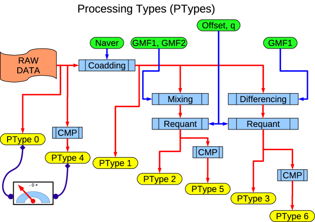
Figure 1: Schematic representation of the scientific on–board processing, processing parameters and processing types for the LFI. The diagram shows the sequence of operations leading to each processing type: coadding, mixing, requantization (Requant) and compression (CMP). A detailed description of the operations is given in [6].

A detailed description of the LFI on–board acquisition chain and the LFI L1 processing is given by [6]. In this work, we use a simplified model of the L1 pipeline in order to present the test methods and procedures applied for the end-to-end tests of the L1 software.

In this model, data in form of time series are generated from various SCI and HK sources (i.e. analog detectors, sensors, registers) on–board the spacecraft and read by the Digital Acquisition Electronics (DAE) which samples the analog signals at discrete times. The analog output of the instrument read by each scientific ADC is either a sequence of interleaved sky and reference–load measures, or a sequence of measures of only sky or only reference–load, depending on the status of the phase–switches associated with each radiometer of the LFI instrument.

The DAE is polled at regular intervals by the on-board processor, the REBA, which runs a pre-processing pipeline, reducing the amount of scientific data generated by the instrument and storing the data in telemetry packets to be sent to ground. A set of 7 extraction points are defined along the REBA pipeline, in order to recover valuable diagnostic data. Each point corresponds to a Processing Type (PType) applied by the REBA on the scientific data (see figure 1). The REBA software can apply concurrently two different PTypes to a single LFI channel. So, in nominal conditions, the instrument will generate just PType 5 data from all of its 44 detectors and short chunks of PType 1 data from a single detector in turn.

In particular, in PType 5 three main processing steps are applied [6]. First, a double difference is performed between two averaged sky and reference–load samples, $\overline{S}_{sky}$ and $\overline{S}_{load}$:

$$P_{1} = \overline{S}_{sky}-\mathrm{GMF1}\cdot\overline{S}_{load}$$ (1)

$$P_{2} = \overline{S}_{sky}-\mathrm{GMF2}\cdot\overline{S}_{load}$$ (2)

where $\mathrm{GMF1}$ and $\mathrm{GMF2}$ are two different gain modulation factors. Then, the two values obtained are requantized converting them into two 16-bit signed integers:

$$Q_{i}=\mathrm{round}\left[\mathrm{q}\cdot\left(P_{i}+\mathrm{Offset}\right)\right]$$ (3)

Finally, the REBA performs a loss-less adaptive arithmetic compression of the data obtained in the previous step. Hence, the REBA pipeline is tunable through a set of processing parameters or REBA parameters: $\mathrm{N_{aver}}$ (the number of consecutive sky or load samples that are averaged), $\mathrm{q}$, $\mathrm{Offset}$, $\mathrm{GMF1}$ and $\mathrm{GMF2}$ [6].

The L1 ground software receives the telemetry packets generated by the instrument. In particular, the scientific telemetry is processed by the TMH/TQL system, which has to handle properly each PType in order to regenerate the time series acquired on-board. The exact steps of the L1 pipeline processing depend on the data source and the PType of each telemetry packet.

4 End-to-end test objectives and methods

To validate the Demonstration Model of the L1 software, developed before the integration and delivery of the LFI instrument, software were developed in order to generate simulated HK telemetry [13] and scientific telemetry [14, 15]. The scope of end-to-end (E2E) tests, instead, is to assess the proper coverage of the requirements by the L1 software and validate its operations by using, as much as possible, the data generated by the testing campaign of the instrument, in particular data gathered from the Qualification Model and the Flight Model of the instrument. The reason is the need to test the software in the most realistic conditions, by performing real instrument operations that allow testing of various operative aspects of the pipeline design. The usage of simulated data has been limited only to cases in which it was not possible to perform a complete E2E test.

Tests have been ordered according to a functional classification of the requirements, consisting of:

1. Handling of raw TM packets:

   1. communication with SCOS,

   2. storing of raw packets,

   3. proper interpretation of primary and secondary headers,

   4. proper commutation of packets according to their purpose, source, service, size and timestamp,

   5. hexadecimal dump of packet content,

   6. other packet related services;

2. Handling of time information;

3. Decompression, decoding and reconstruction of scientific packets content;

4. Decoding and reconstruction of HK packets content;

5. TOIs generation;

6. Graphical displays;

7. On-the-fly software analysis;

8. Other services.

There are overlaps between some of the classes. In particular, the first 4 classes are strictly connected, allowing a minimization of the number of tests. Classes from 6 to 8 can be tested by comparing their output directly with the TOIs rather than the input signals. Test procedures have been defined to cover one or more test cases of the L1 E2E test plan and formalized into a set of test controls sheets.

4.1 Scientific data processing: testing method and setup

Figure 1 suggests a possible testing strategy, i.e. comparison testing. This is based on the comparison of data taken with different PTypes. In the figure, a small gauge is connected to PType 0 and PType 4 data. The gauge represents the L1 software receiving PType 0 and PType 4 data from the same data source (detector), processing and comparing them. Given that the compression/decompression is a completely loss–less process, a correct result would be PType 4 data, after decompression, to be identical to the corresponding PType 0 data.

More generally, even an absolute testing is required to assure that data are properly acquired, processed, received, reconstructed, displayed and stored by the pipeline as a whole. This is obtained by acquiring a signal of well known properties (period, shape, amplitude, voltage levels, duty cycles) at the DAE analog gates, processing it through the whole system and comparing it with the output by using a suitable set of metrics. Depending on the type of test, identity between input and output or statistical agreement among them have been used as a criteria to assess the success or failure of the test. As a by product, this kind of testing is able to detect potential problems in the on–board acquisition electronics and software.

Figure 2: Hardware setup during the end-to-end tests.

Figure  2 represents the complete acquisition chain of LFI during the E2E tests. The signal is injected through an oscilloscope probe at the input of a DAE pin corresponding to the detector to be tested. The signal is generated through a stabilized, digital function generator, and it is monitored by a digital oscilloscope connected to the signal generator by a high impedance probe. Monitoring is required to asses that the signal produced by the function generator matches the required characteristics. In some tests, the same signal has been distributed to different inputs by a signal distributor.

To analyze the test data, it would have sufficed to correlate the output signal with the input signal, but practically it was difficult to record the input signal separately. So, the statistical properties of the output have been compared to the properties of the input measured by the oscilloscope and characterized by the following parameters: the shape, the period $T$, the duration of the high state $T_{\mathrm{up}}$, the duration of the low state $T_{\mathrm{down}}$, the duty cycle $\delta_{\mathrm{cycle}}=T_{\mathrm{up}}/T$, the low state voltage $V_{\mathrm{low}}$, the high state voltage $V_{\mathrm{up}}$, and the peak-to-peak amplitude $A=V_{\mathrm{up}}-V_{\mathrm{low}}$. The source of the signal shall ensure that all of these parameters are known accurately, a good S/N (at least 20), that the signal fits the range of voltages acceptable to the input gate at which it is connected, that it is stable, within the quantization step of the ADC converter, and that $V_{\mathrm{low}}$, $V_{\mathrm{up}}$, $T_{\mathrm{up}}$, and $T_{\mathrm{down}}$ are adjustable within a wide range of values.

For each test, the general procedure has been the following:

1. the signal generator has been plugged to the DAE input corresponding to the channel to be tested;

2. the signal generator has been set-up for the type of signal needed for the specific test. The oscilloscope has been used to check the signal properties;

3. telecommands have been sent to the DAE to set the proper acquisition setup;

4. the DAE acquisition has been started keeping the generator off,

5. after about 5 seconds the generator has been switched on for the time required by the test;

6. the generator has been switched off and after about 5 seconds the acquisition has been stopped.

In this procedure, the steps in which the signal generator is switched on and off have been used to allow a semiautomatic identification of the start and end time of each test within the timelines generated by the L1 software. The setup of each test has been recorded by documenting the cabling, the signal generator setup, keeping screenshots of the SCOS displays and archiving the log generated through the TQL where each test phase has been annotated. The subsequent data analysis has been carried out off–line.

5 Data analysis procedures

5.1 Software

An analysis toolkit, OCA (On-board Computing Analysis), implemented in the Interactive Data Language (IDL) and in C++, with additional off-the-shelf freeware libraries and applications, has been developed to analyze the test data. OCA provides simple analysis methods and automated reporting. The use of this toolkit assures repeatability of test analysis.

In particular, OCA allows the processing of the raw telemetry archive generated by the TMH together with the intermediate products of the pipeline and the corresponding log files. It provides functions to: decode the packets content, in particular the On-Board Time (OBT) and the acquisition parameters stored in the tertiary header of the scientific packets; scan the TOI archive and split tests into frames; detect pulses of known shapes within packets or TOIs; identify the source packet from which a given sample was extracted; perform comparisons between the TOIs and corresponding scientific packets. Moreover, it simulates the conversion of PType 1 data into PType 2 data, to verify the correct processing of these data types [12].

5.2 On-line and off-line analysis

Depending on the scope of the test, data analysis was performed on-line and off-line. On-line analysis has been carried out for all of the live operations of the L1 software. For instance, we tested on-line the TQL function which generates an hexadecimal dump of the packets by comparing it with the same function performed by SCOS, the function which monitors the REBA parameters currently in use, the graphical displays and the FFT computation. Most of the other functionalities, such as OBT and TOI reconstruction, have been tested off-line.

The first group of tests have covered the basic functionalities. In particular, we checked that all the TM packets are received and stored, that each packet header is properly handled in the packets archive, the proper interpretation of primary, secondary and tertiary headers, that packets are properly registered, i.e. grouped according to the data source and processing type and converted into TOIs. In this group of tests, the checking of the TOI creation was focused on testing the proper mapping between the TM packets and the raw samples contained in the TOIs.

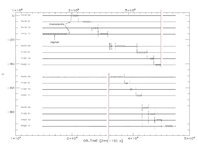
Figure 3: Simplified scheme of registration for 16 of the 44 LFI channels. Note that the vertical scale is in volts, but each plot is vertically shifted for graphical purposes. For the same reason the time line is split and shifted back at the level of the vertical red–line.

The test checking for proper registration of scientific packets is illustrated in figure 3. In that test, the acquisition was kept running while the signal generator was connected in turn to each analog input of the DAE. The data analysis looks for erroneous activation of unplugged channels and/or lack of activation of the plugged ones. It is evident that the presence of a signal in one of the TOIs excludes signals in others (apart from short transients, corresponding to the plugging/unplugging operations) and that there are no holes in the data.

5.3 Signal reconstruction

A more advanced test procedure and analysis was required to test the OBT reconstruction and the conversion to physical units. Ideally, those two elements of the processing should have been tested separately. In practice, time handling is connected to the identification of features in the signal, such as the period between subsequent peaks or the reconstruction of the phase information, which are obviously connected to a proper signal reconstruction.

After having identified the region where the signal generator is “on”, a Lomb-Scargle Periodogram (LSP) is applied to assess the period of the signal as measured by the OBT time scale. The LSP has the advantage, over the FFT, of being robust against perturbations introduced by erroneous inclusions of short no-signal zones or interruptions in the data. The LSP is automatically scanned looking for the peak with the highest power, giving a first approximation of the period. The period is further refined by fitting the LSP peak with a ${\mathrm{sinc}}(x)$ with two free parameters: the difference in the peak period $\delta p$ with respect to the approximate period and the peak normalization. The fitting procedure estimates also the error in the two free parameters. The error in $\delta p$ is taken as the error in the period estimate.

The phases and amplitude determination depends on the wave shape. For square waves, $V_{\mathrm{low}}$, $V_{\mathrm{high}}$, amplitudes and phases are determined by using a $\chi^{2}$ fitting combined with a phase–folded diagram. The $\chi^{2}$ is computed between the model calculated for a given tentative phase, $\Phi$, and the signal. A fine-grained grid of phases is explored and the minimum $\chi^{2}$ is used to assess the best phase.

The model for the triangular wave assumes that the transition between the growing and the decreasing ramp is instantaneous. The peak-to-peak amplitude for the triangular wave is determined by the moments of the cumulative distribution function of the samples. In particular

$$A=\sigma_{\mathrm{triangular}}\sqrt{12}.$$ (4)

In this way, the determination of the peak-to-peak amplitude is decoupled from the determination of period and phase. The phase is again determined by the $\chi^{2}$ method used for the square waves.

5.4 PType comparison

Since the REBA is able to process data from the same detector with two different processing types in parallel, this functionality was used to perform a comparison between the TOIs of the same signal obtained from two PTypes. An example is given in figure 4, where data acquired with PType 1 have been compared with the same data acquired with PType 5. The example concerns a test where a square wave with a period of 1 second, peak-to-peak amplitude of about 0.84 V and duty cycle $\delta_{\mathrm{cycle}}=0.25$ has been used; phase switching was left off, so each resulting TOI contains only sky samples. The figure covers the analysis performed on data from feed-horn 28, radiometer 0 and detector 0 only. The processing parameters used are: $\mathrm{N_{aver}}$=126, $\mathrm{GMF1}$=1, $\mathrm{GMF2}$=-1, $\mathrm{Offset}$=0, $\mathrm{q}$=1.

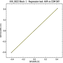
(a)

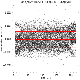
(b)

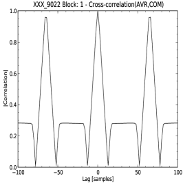
(c)

Figure 4: Frame a) Comparison of two different processing types (PType5 and PType1) applied to the same data stream. Points are the original data, the yellow line is the ideal relation. Frame b) Processing error introduced by PType5. The red lines represent the average expected processing error and the $\pm 1$ band. Note that the distribution of this error is visibly not Gaussian. Besides, digitization of data is very tiny and the distribution of noise in the region where the signal generator is off is not uniform. Frame c) Cross-correlation test between PType 5 and PType 1.

In particular, the first frame in figure 4 shows a correlation plot of PType 5 (COM) versus PType 1 (AVR) data. As it is possible to see, the correlation is perfectly linear. A more refined test is the evaluation of the processing error (or quantization error) introduced by the PType 5 transformations. It is defined as:

$$\epsilon_{q}=V_{\mathrm{PType5}}-V_{\mathrm{PType1}}$$ (5)

where $V_{\mathrm{PType1}}$ and $V_{\mathrm{PType5}}$ are, respectively, the measures obtained acquiring the data at the same time by using both the 1 and 5 processing modes. The error, compared to the expectation from processing parameters, is plotted in the second frame of figure 4. It shows the effect of the digitization which, in this case, is very tiny. Some structure in the noise is clearly present, especially at the left and right side where the signal was off. Moreover, the noise does not follow a Gaussian distribution.

An additional test performed is the cross-correlation index, $\mathcal{C}^{I}_{1,5}=\rho_{1,5}(0)$, between PType 1 and PType 5. We evaluated the cross-correlation for a range of time lags. The cross-correlation is calculated by shifting the TOI obtained from PType 5 data with respect to the one obtained from PType 1 data by a lag of $\Delta t$, taking $\Delta t$ = 0 as the case for overlapping PType 5 with PType 1.

The results obtained always showed $\rho_{1,5}(\Delta t)\leq\rho_{1,5}(0)$. The third frame of figure 4 shows an example of such case for one of the tests, where we have obtained $1-\mathcal{C}^{I}_{1,5}=1.81\cdot 10^{-8}$.

5.5 OBT reconstruction

Testing for proper handling of time information is critical since time series are matched by comparing samples with the same OBT. In particular the matching of the OBTs is used to correlate scientific time series with HK time series. OBTs are also used to correlate scientific data acquired by using different PTypes from the same detector and estimate the quantization error $\epsilon_{q}$.

In particular, when testing the OBT reconstruction, we consider the following type of anomalies: gaps between the last sample of a packet and the first sample of the subsequent one; overlaps between the last samples of a packet and the first samples of the subsequent one; the presence of duplicated packets; possible errors in estimating the time scale (sampling step) and the zero point of the OBT.

The test procedures for the OBT reconstruction consist in:

1. checking whether the sampling rate derived from OBT is consistent with $N_{aver}$;

2. checking whether there are defects (holes) in the OBT;

3. verifying that holes (if present) in the OBT are just due to acquisition stops;

4. measuring periods, duty-cycles of signals and checking if they are consistent with the periods imposed by the signal generator;

5. checking that the correlation between the OBT of a packet and the OBT in the corresponding TOIs is correct;

6. correlating two different PTypes applied to the same signal.

5.5.1 Anomalies in the sampling rate

The sampling period for PType 1, 2, 3, 5 and 6 data shall be

$$\tau_{\mathrm{sampling}}=\frac{\mathrm{N_{aver}}}{8192}\;\mathrm{seconds}.$$ (6)

For any pair of consecutive samples $[i,i+1]$, where $i=0$ denotes the first sample in the TOI, the OBT should be a monotonically increasing quantity; so, denoting with $t^{\mathrm{ob}}$ the OBT and having

$${\tau^{\prime}}_{\mathrm{sampling},i}=t^{\mathrm{ob}}_{i+1}-t^{\mathrm{ob}}_{i}$$ (7)

then for any $i$, ${\tau^{\prime}}_{\mathrm{sampling},i}\equiv\tau_{\mathrm{sampling}}$. Hence, a simple histogram of ${\tau^{\prime}}_{\mathrm{sampling},i}$ allows discovering the presence of anomalies, i.e. cases in which ${\tau^{\prime}}_{\mathrm{sampling},i}\neq\tau_{\mathrm{sampling}}$. Table 1 gives a summary of the possible anomalies and their most likely source. Gaps in the timelines are allowed when the acquisition is stopped.

Table 1: Diagnostic of $\tau_{\mathrm{sampling}}$.

Case			Diagnostic
${\tau^{\prime}}_{\mathrm{sampling},i}$	$\leq$	$0$	repeated packets or reset in the on–board clock
${\tau^{\prime}}_{\mathrm{sampling},i}$	$<$	$\tau_{\mathrm{sampling}}$	overlapping of packets or erroneous decrease in $N_{\mathrm{aver}}$
${\tau^{\prime}}_{\mathrm{sampling},i}$	$=$	$\tau_{\mathrm{sampling}}$	the nominal condition
${\tau^{\prime}}_{\mathrm{sampling},i}$	$>$	$\tau_{\mathrm{sampling}}$	gap in the acquisition or erroneous increase in $N_{\mathrm{aver}}$

The test is complemented by cross-checking the OBT in the packet secondary header and the corresponding OBTs in the TOIs.

In an early test, a problem discovered by this method was an inconsistent distribution of $\tau_{\mathrm{sampling}}$ for PTypes 1 and 2 when the phase switch was off. They were a factor of 2 too large. This occurred because of an incorrect handling of the OBTs by the TMH in this instrument configuration. After fixing the problem the test was successfully repeated. No defects or unexplained gaps in the OBT have been found when the phase switch was on.

Another example of a problem discovered and corrected by looking at an erroneous OBT reconstruction was the case of an early attempt to carry out acquisition of PType 2 and 5 together. In that case, the TMH did not register properly the PType 5 data since the data of both PTypes were stored in the same TOI instead of storing them into separate timelines. Since PType 5 packets are generated at a rate of about 1/6 of PType 1, the OBT apparently jumped back about every 6 PType 1 packets.

5.5.2 Packet-Peak correlation

Packet-Peak correlation is a method to assess the use of the OBT as a way to correlate packets to events occurring in different time lines. The measure of Packet-Peak correlation is assessed by measuring the time interval between the first peak contained in the packet, $t^{\mathrm{ob}}_{\mathrm{peak}}$, and the time stamp of the packet, $t^{\mathrm{ob}}_{\mathrm{packet}}$.

For square waves, the peak position is defined as the OBT for which $\mathrm{folding}(t^{\mathrm{ob}}_{\mathrm{peak}})=\delta_{\mathrm{cycle}}/2$ then a square wave “belongs” to a packet if $t^{\mathrm{ob}}_{\mathrm{packet}}\leq t^{\mathrm{ob}}_{\mathrm{peak}}.$

Then, the packet-to-peak correlation

$$\Delta T_{\mathrm{pck}-\mathrm{peak}}=t^{\mathrm{ob}}_{\mathrm{peak}}-t^{\mathrm{ob}}_{\mathrm{packet}}$$

can be easily predicted when the period of production of packets and the period of the square wave is known. In particular, for uncompressed data, packets are generated with period:

$$\tau_{\mathrm{pck}}=\frac{\mathcal{N}_{\mathrm{pck}}\mathrm{N_{aver}}}{f_{\mathrm{sampling}}}\;\mathrm{seconds},$$ (8)

where $\mathcal{N}_{\mathrm{pck}}$ is the number of samples in the packet: 490 for any uncompressed PType, except PType 1 for which $\mathcal{N}_{\mathrm{pck}}=245$. The deviation of $\Delta T_{\mathrm{pck}-\mathrm{peak}}$ from the predicted value is measured by:

$$\mathcal{C}T_{\mathrm{pck}-\mathrm{peak}}=\frac{\left|\Delta T_{\mathrm{pck}-\mathrm{peak}}-\Delta T^{\mathrm{Calc}}_{\mathrm{pck}-\mathrm{peak}}\right|}{\tau_{\mathrm{pck}}},$$ (9)

where $\Delta T^{\mathrm{Calc}}_{\mathrm{pck}-\mathrm{peak}}$ is the $\Delta T_{\mathrm{pck}-\mathrm{peak}}$ predicted. The test fails if $\mathcal{C}T_{\mathrm{pck}-\mathrm{peak}}>1/(10^{3}\mathrm{N_{aver}})\approx 10^{-6}$. In no cases a packet–peak correlation worst than $\mathcal{C}T_{\mathrm{pck}-\mathrm{peak}}<10^{-11}$ have been detected.

5.5.3 Period determination

An erroneous reconstruction of the OBT would result in an erroneous estimate in the period of the signal as measured by using the LSP. Given that the OBT of the packets is given in seconds, with a 16 bits accuracy for the fractional part, the maximum error in determining the period should be of the order of $10^{-4}$ seconds.

To check for this case we did various tests with different combinations of signal periods, amplitudes and $\mathrm{N_{aver}}$. Periods in the measured waveforms have been fitted by using the LSP together with phase folding as explained in Sect. 5.3. Typically, accuracies better than $9\times 10^{-5}$ sec have been obtained.

5.6 ADU conversion

The use of a signal generator allows conversion from ADU (Analog to Digital Unit) to physical units (Volts) to be tested. A linear fit between the fitted $V_{fit}$ and the generator values $V_{generator}$,

$$V_{fit}=\textrm{Intercept}+\textrm{Slope}\cdot V_{generator},$$ (10)

has been performed. Pearson statistics have been used as a way to assess linearity. The fit has been performed either comparing the High levels, the Low levels or both. The ideal case would be:

$$\textrm{Intercept}=0,\textrm{Slope}=1,\textrm{Pearson}=1.$$ (11)

Typically, we obtained $|\textrm{Intercept}|<5\times 10^{-3}$, $|1-\textrm{Slope}|<10^{-2}$ and $|1-\textrm{Pearson}|<10^{-4}$.

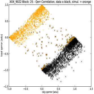
(a)

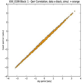
(b)

Figure 5: Frame a) Distribution of quantization errors for sky vs quantization errors for load for true PType 5 data (black crosses) and the simulated processing (orange crosses). Frame b) The same test performed on another data set after the bug on the on-board software was corrected.

5.7 Quantization errors

Comparing PType 5 and PType 1 data allowed discovering anomalies in the quantization error. Tests have shown that the differences between PType 1 and PType 5 are small and compatible with the expected quantization error (depending on the REBA processing parameters applied). However, in a first run of these tests, in some cases it was noted that the distribution of quantization errors did not follow the expectation exactly, since they were not symmetrically distributed around zero.

A more detailed analysis is shown in Fig 5a, where the processing leading to PType 5 generation from PType 1 data has been carried out according to the documented on-board algorithm. The figure shows a scatter plot of sky vs. load processing error. It is possible to see that the expected processing error is not distributed as the real one. After the analysis, it was concluded that it was due to a bug in the on-board software, when rounding negative values in the quantization step. The bug was subsequently corrected and a second run of the tests has shown that the quantization error now follows the expectation (Fig 5b).

5.8 Decompression

PType 2 and PType 5 data where acquired together. Data from PType 5 processing are compared with data from PType 2 processing. No differences were revealed between PType 2 and PType 5 data. The compression/decompression procedure passed this test.

6 Housekeeping processing validation using a known pattern

Unlike the case of the scientific telemetry, it wasn’t possible to inject known signals into the HK packets directly through the DAE/REBA chain. The HK parameters are heterogeneous and include temperature sensor values, current consumptions, register values, switch statuses. Different parameters are grouped by hardware unit, sampling frequency and service purpose and stored in the same HK packet.

The structure of the HK telemetry packets strictly follows the rules of the ESA Packet Utilization Standard (PUS). According to the PUS, each field in a telemetry HK packet is either a parameter field containing a parameter value or a structured field containing several parameter fields organized according to a set of rules. The PUS permits the structure of a HK packet to be defined by specifying, for each parameter within the packet, the offset with respect to the packet primary header, the parameter type code and format code and the offset of the subsequent samples of the parameter.

The HK packet structure definitions are provided in an Interface Control Document (ICD) of the instrument and then mapped in the SCOS Mission Information Base (MIB), a set of ASCII tables containing all the monitoring parameters characteristics and location within each telemetry packet and the telecommands characteristics. Both the SCOS system and the TMH/TQL system of the LFI-DPC import the packet structure definitions from the MIB tables.

In order to test the decoding and reconstruction of the HK packets content, an Housekeeping Validation System (HVS) has been developed to manipulate the binary representation of an HK packet with the goal of generating packets with known parameter values starting from a set of real HK packets.

6.1 The HVS system

The HVS system has been developed to test the correct processing of each HK packet type. Packets of the same type have an identical structure and are identified by 4 fields: the Application ID (APID), the service Type and Subtype, contained in the packet primary and secondary headers, and the Structure ID (SID), contained in the first two bytes of the data segment.

For each HK packet type and parameter within it, the HVS system creates a predefined pattern of values. It iterates over all the samples of the parameter, setting to 1 one bit a time. Hence, for each sample, only a single bit of a single parameter has value 1 while all the other bits have value 0. This implies that for a given HK packet type, each parameter in turn takes increasing power of 2 values. One of the purposes of this pattern is to verify that in the TMH/TQL system the offset and the length of each parameter has been correctly defined.

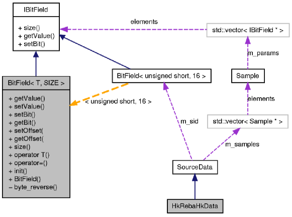
Figure 6: Class diagram of the core components of the HVS system.

Figure 6 shows the class diagram of the components of the HVS system which build an HK packet structure. The data segment (source data) of a packet starts with the SID field, used to identify the packet type. Then a sequence of samples follow. Each sample is composed of a sequence of different parameters. A parameter is represented by a bit field (BitField template class) specifying the size in bits of the parameter, its raw value type and the offset of the parameter within the sample. The BitField class inherits from a pure abstract class, the IBitField class, which is used to iterate over all parameters, independently of their concrete type, to set each bit value.

The HVS system is able to increase the number of packets in the input dataset, introducing new packets with coherent OBT, sample time and source sequence count values and keeping constant the proportion of each packet type within the dataset. With this feature, we have produced a dataset corresponding to an acquisition lasting 6 days. This was necessary to apply the pattern of values to packets with a low frequency (64 seconds) and containing a large number of HK parameters.

The dataset generated by the HVS system is then processed by the TMH in order to generate the HK timelines. For each packet type, the parameter values of the input dataset are compared with the corresponding TOIs generated by the TMH in order to highlight possible discrepancies.

6.2 HK tests results

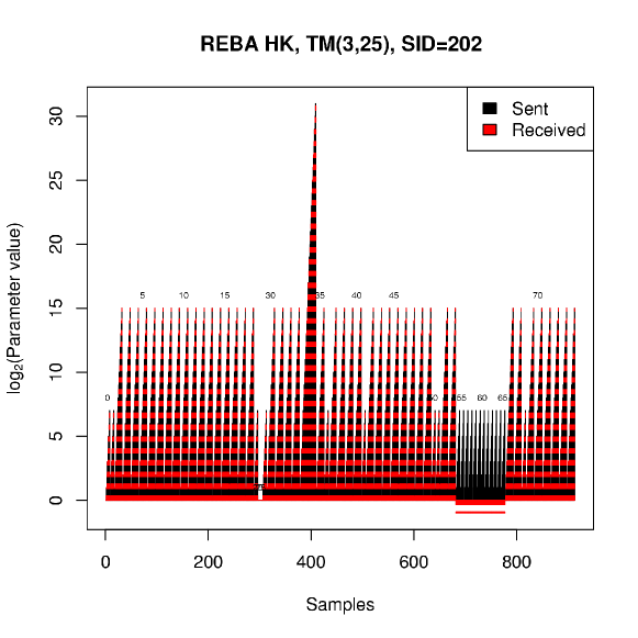
Figure 7: Comparison between the HK parameters values in the HVS generated dataset (black) with values in the corresponding TOIs (red) for the REBA HK telemetry packet.

Tests performed with the HVS system have highlighted an error in the handling of two HK telemetry packets types, the REBA HK packet and the REBA Diagnostic HK packet, which have a common structure. The problem is shown in figure 7 for the REBA HK packet: it represents a plot of the HK parameter values in the dataset generated by the HVS system (black) and the corresponding TOIs generated by the TMH system (red). The parameters are ordered according to their position in the packet (denoted by the number on the top of each peak). The “sample” axis is the location in the test sequence where that sample is tested with the given value. The problem with the registration of the HK parameters is evidenced by the anomalous distribution of red points around the sample 700. This test has proved that there was a discordance between the ICD describing the packets structure for LFI and their mapping in the SCOS 2000 MIB [10]. After this analysis, the offsets of the involved parameters were corrected in the MIB tables by the instrument team and successfully checked with a rerun of this test.

7 Conclusions

The Level 1 software system of Planck/LFI, which is a critical component of the Planck science ground segment, has been validated by applying the ESA standards for software verification and validation. The tests have been designed to recreate the most realistic operational conditions, using telemetry directly generated by the instrument, whenever possible. An additional effort was needed to develop testing and analysis tools devoted to the end-to-end tests. Some relevant bugs have been identified in the first run of the tests, performed on the Qualification Model of the software, and rapidly fixed. The Flight Model of the Level 1 has successfully passed the end-to-end validation tests and has been adopted for the entire LFI calibration tests campaign and the subsequent Planck integration tests.

- [1] ESA Publications, ESA Software Engineering Standards, ESA Procedures Standards and Specifications, PSS-05-0 (1991), \hrefftp://ftp.estec.esa.nl/pub/wm/wme/bssc/PSS050.pdfftp://ftp.estec.esa.nl/pub/wm/wme/bssc/PSS050.pdf.
- [2] ESA Publications, Guide to software verification and validation, ESA Procedures Standards and Specifications, PSS-05-10 (1995) \hrefftp://ftp.estec.esa.nl/pub/wm/wme/bssc/PSS0510.pdfftp://ftp.estec.esa.nl/pub/wm/wme/bssc/PSS0510.pdf.
- [3] ECSS Standard, Space product assurange - Quality assurance, European Cooperation for Space Standardization, ECSS-Q-ST-20C, 2008
- [4] F. Pasian et al., Planck/LFI Pipeline – The Demonstration Model, Astron. Data Anal. Soft. Sys. XIV 347 (2005) 609.
- [5] A. Mennella et al., Calibration and testing of the Planck-LFI QM instrument, Space Telescopes and Instrumentation I: Optical, Infrared, and Millimeter, \hrefhttp://dx.doi.org/10.1117/12.669408Proc. SPIE 6265 (2006) 62650G.
- [6] A. Zacchei et al., Level 1 on ground telemetry handling in Planck LFI, \hrefhttp://dx.doi.org/10.1088/1748-0221/4/12/T120192009 JINST 4 T12019.
- [7] M. Frailis et al., Level 1 core software testing for Planck/LFI, in Proceedings of CMB and Physics of the Early Universe, April 22-26, 2006 Ischia, Italy, \posPoS(CMB2006)035
- [8] L. Popa, M. Maris, F. Bottega and F. Pasian, Planck LFI - DPC Software Integration and Testing Plan, Astronomical Observatory of Trieste, Tech. Report, PL-LFI-OAT-PL-006 (2006).
- [9] M. Maris, M. Frailis, Planck LFI - Test Plan for the TMH/TQL software, Astronomical Observatory of Trieste, Tech. Report, PL-LFI-OAT-PL-009 (2006).
- [10] M. Maris, M. Frailis, Planck LFI - Test Report on the TMH/TQL (QM and FM) by Using a Known Signal Test data, Astronomical Observatory of Trieste, Tech. Report, PL-LFI-OAT-RP-17 (2008).
- [11] I. Somerville, Software Engineering, Addison Wesley, 8th edition (2006).
- [12] M. Maris et al., Optimization of PLANCK/LFI on-board data handling, \hrefhttp://dx.doi.org/10.1088/1748-0221/4/12/T120182009 JINST 4 T12018. .
- [13] A. Zacchei et al., HouseKeeping and Science Telemetry: the case of Planck/LFI, Mem. S.A.It. Suppl. 3 (2003) 331, \hrefhttp://sait.oat.ts.astro.it/MSAIS/3/PDF/331.pdfhttp://sait.oat.ts.astro.it/MSAIS/3/PDF/331.pdf.
- [14] M. Maris et al., A scientific Telemetry generator for the Planck/LFI flight simulator, Astronomical Observatory of Trieste, Tech. Report,PL-LFI-OAT-TN-17 (2001).
- [15] S. Fogliani, M. Malaspina et al., Planck/LFI: management of telemetry, Mem. S.A.It. 74 (2003) 470, \hrefhttp://sait.oat.ts.astro.it/MSAIt740203/PDF/2003MmSAI..74..470F.pdfhttp://sait.oat.ts.astro.it/MSAIt740203/PDF/2003MmSAI..74..470F.pdf.