A WKB–like approach to Unruh Radiation

Abstract

Unruh radiation is the thermal flux seen by an accelerated observer moving through Minkowski spacetime. In this article we study Unruh radiation as tunneling through a barrier. We use a WKB–like method to obtain the tunneling rate and the temperature of the Unruh radiation. This derivation brings together many topics into a single problem – classical mechanics, relativity, relativistic field theory, quantum mechanics, thermodynamics and mathematical physics. Moreover, this gravitational WKB method helps to highlight the following subtle points: (i) the tunneling rate strictly should be written as the closed path integral of the canonical momentum; (ii) for the case of the gravitational WKB problem, there is a time–like contribution to the tunneling rate arising from an imaginary change of the time coordinate upon crossing the horizon. This temporal contribution to the tunneling rate has no analog in the ordinary quantum mechanical WKB calculation.

I Introduction

The radiation that arises from placing a quantum field in a background metric with a horizon is a well known phenomenon at the boundary between field theory and general relativity. The first example of this effect was Hawking radiation hawking , where a Schwarzschild black hole radiates with a thermal spectrum at the expense of the black hole’s mass. Another example is Hawking–Gibbons radiation gibbons , i.e., the thermal radiation seen by an observer in de Sitter spacetime. In this paper we focus on Unruh radiation unruh – the radiation seen by an observer moving with a constant acceleration through vacuum. The original methods used to calculate these effects used quantum field theory at a level which is beyond most undergraduates or beginning graduate students. In reference hawking, , Hawking gave a heuristic picture for the radiation in terms of “tunneling” of virtual particles across the horizon. After a span of twenty five years, mathematical details were added to this picture kraus ; padman ; parikh1 ; parikh2 . In these works, the action for a particle which crosses the horizon of some spacetime (e.g., the Schwarzschild spacetime for the case of Hawking radiation) was calculated and found to have an imaginary part coming from a contour integration. The exponential of this imaginary piece was compared to a Boltzmann distribution, which allowed one to determine the temperature of the radiation. The simplicity of this gravitational WKB method makes it easy to calculate Hawking like radiation for the case of other metrics (e.g. Reissner–Nordstrom parikh1 , de Sittersekiwa ; volovik ; medved ; temporal , Kerr and Kerr–Newmann kerr ; kerr2 , Unruh unruhPLB ). Additionally, one could easily incorporate tunneling particles with different spins mann and one could (in a simplified way) begin to take into account back reaction effects on the metric parikh1 ; parikh2 ; vagenas .

In reference donoghue, , Unruh radiation is derived using purely quantum mechanical arguments. However, the reader needs to know the quantized radiation field, and the mathematical steps in the derivation are more involved as compared to the approach presented here. In comparison with reference donoghue, , the gravitational WKB–like method is mathematically simple while at the same time it provides a clear physical picture for the origins of the radiation. In this article, this WKB–like method is presented in a pedagogical manner for the case of the Rindler spacetime (the metric seen by an observer who undergoes constant proper acceleration) and Unruh radiation. The reason for choosing Rindler spacetime is that it is the simplest spacetime in which this effect occurs. Furthermore, because of the strong equivalence principle (i.e., locally, a constant acceleration and a gravitational field are observationally equivalent), the Unruh radiation from Rindler spacetime is the prototype of this type of effect. Also, of all these effects – Hawking radiation, Hawking–Gibbons radiation – Unruh radiation has the best prospects for being observed experimentally jackson ; bell ; akhmedov1 ; retz .

This derivation of Unruh radiation draws together many different areas of study: (i) classical mechanics via the Hamilton–Jacobi equations; (ii) relativity via the use of the Rindler metric; (iii) relativistic field theory through the Klein–Gordon equation in curved backgrounds; (iv) quantum mechanics via the use of the WKB–like method applied to gravitational backgrounds; (v) thermodynamics via the use of the Boltzmann distribution to extract the temperature of the radiation; (vi) mathematical methods in physics via the use of contour integrations to evaluate the imaginary part of the action of the particle that crosses the horizon. Thus this single problem serves to show students how the different areas of physics are interconnected.

Also, through this example we will highlight some subtle features of the Rindler metric and the WKB method which are usually overlooked. In particular, we show that the gravitational WKB amplitude has a contribution coming from a change of the time coordinate from crossing the horizon temporal . This temporal contribution is never encountered in ordinary quantum mechanics, where time acts as a parameter rather than a coordinate.

II Rindler spacetimes

In this section we introduce and discuss some relevant features of Rindler spacetime – the spacetime seen by an observer moving with constant proper acceleration through Minkowski spacetime. The Rindler metric can be obtained by starting with the Minkowski metric, i.e., $ds^{2}=-dt^{2}+dx^{2}+dy^{2}+dz^{2}$, where we have set $c=1$, and transforming to the coordinates of the accelerating observer. We take the acceleration to be along the $x$–direction, thus we only need to consider a 1+1 dimensional Minkowski spacetime

$$ds^{2}=-dt^{2}+dx^{2}~{}.$$ (1)

Using the Lorentz transformations (LT) of special relativity, the worldlines of an accelerated observer moving along the $x$–axis in empty spacetime can be related to Minkowski coordinates $t$, $x$ according to the following transformations

$$\begin{split}t&=(a^{-1}+x_{R})\sinh(at_{R})\\ x&=(a^{-1}+x_{R})\cosh(at_{R})~{},\end{split}$$ (2)

where $a$ is the constant, proper acceleration of the Rindler observer measured in his instantaneous rest frame. One can show that the acceleration associated with the trajectory of (2) is constant since $a_{\mu}a^{\mu}=(d^{2}x_{\mu}/dt_{R}^{2})^{2}=a^{2}$ with $x_{R}=0$. The trajectory of (2) can be obtained using the definitions of four–velocity and four–acceleration of the accelerated observer in his instantaneous inertial rest frame MTW . Another derivation of (2) uses a LT to relate the proper acceleration of the non–inertial observer to the acceleration of the inertial observer rindlerSR . The text by Taylor and Wheeler taylor also provides a discussion of the Rindler observer.

The coordinates $x_{R}$ and $t_{R}$, when parametrized and plotted in a spacetime diagram whose axes are the Minkowski coordinates $x$ and $t$, result in the familiar hyperbolic trajectories (i.e., $x^{2}-t^{2}=a^{-2}$) that represent the worldlines of the Rindler observer.

Differentiating each coordinate in (2) and substituting the result into (1) yields the standard Rindler metric

$$ds^{2}=-(1+ax_{R})^{2}dt_{R}^{2}+dx_{R}^{2}~{}.$$ (3)

When $x_{R}=-\frac{1}{a}$, the determinant of the metric given by (3), $det(g_{ab})\equiv g=-(1+ax_{R})^{2}$, vanishes. This indicates the presence of a coordinate singularity at $x_{R}=-\frac{1}{a}$, which can not be a real singularity since (3) is the result of a global coordinate transformation from Minkowski spacetime. The horizon of the Rindler spacetime is given by $x_{R}=-\frac{1}{a}$.

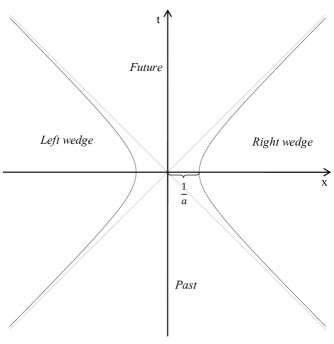
Figure 1: Trajectory of the Rindler observer as seen by the observer at rest.

In the spacetime diagram shown above, the horizon for this metric is represented by the null asymptotes, $x=\pm t$, that the hyperbola given by (2) approaches as $x$ and $t$ tend to infinity BD . Note that this horizon is a particle horizon, since the Rindler observer is not influenced by the whole spacetime, and the horizon’s location is observer dependent visser .

One can also see that the transformations (2) that lead to the Rindler metric in (3) only cover a quarter of the full Minkowski spacetime, given by $x-t>0$ and $x+t>0$. This portion of Minkowski is usually labeled Right wedge. To recover the Left wedge, one can modify the second equation of (2) with a minus sign in front of the transformation of the $x$ coordinate, thus recovering the trajectory of an observer moving with a negative acceleration. In fact, we will show below that the coordinates $x_{R}$ and $t_{R}$ double cover the region in front of the horizon, $x_{R}=-\frac{1}{a}$. In this sense, the metric in (3) is similar to the Schwarzschild metric written in isotropic coordinates. For further details, see reference visser, .

There is an alternative form of the Rindler metric that can be obtained from (3) by the following transformation:

$$(1+a\,x_{R})=\sqrt{|1+2\,a\,x_{R^{\prime}}|}~{}.$$ (4)

Using the coordinate transformation given by (4) in (3), we get the following Schwarzschild–like form of the Rindler metric

$$ds^{2}=-(1+2\,a\,x_{R^{\prime}})dt_{R^{\prime}}^{2}+(1+2\,a\,x_{R^{\prime}})^{-1}dx_{R^{\prime}}^{2}~{}.$$ (5)

If one makes the substitution $a\rightarrow GM/x_{R^{\prime}}^{2}$ one can see the similarity to the usual Schwarzschild metric. The horizon is now at $x_{R^{\prime}}=-1/2a$ and the time coordinate, $t_{R^{\prime}}$, does change sign as one crosses $x_{R^{\prime}}=-1/2a$. In addition, from (4) one can see explicitly that as $x_{R^{\prime}}$ ranges from $+\infty$ to $-\infty$ the standard Rindler coordinate will go from $+\infty$ down to $x_{R}=-1/a$ and then back out to $+\infty$.

The Schwarzschild–like form of the Rindler metric given by (5) can also be obtained directly from the $2$–dimensional Minkowski metric (1) via the transformations

$$\begin{split}t&=\frac{\sqrt{1+2ax_{R^{\prime}}}}{a}\sinh(at_{R^{\prime}})\\ x&=\frac{\sqrt{1+2ax_{R^{\prime}}}}{a}\cosh(at_{R^{\prime}})\end{split}$$ (6)

for $x_{R^{\prime}}\geq-\frac{1}{2a}$, and

$$\begin{split}t&=\frac{\sqrt{|1+2ax_{R^{\prime}}|}}{a}\cosh(at_{R^{\prime}})\\ x&=\frac{\sqrt{|1+2ax_{R^{\prime}}|}}{a}\sinh(at_{R^{\prime}})\end{split}$$ (7)

for $x_{R^{\prime}}\leq-\frac{1}{2a}$. Note that imposing the above conditions on the coordinate $x_{R^{\prime}}$ fixes the signature of the metric, since for $x_{R^{\prime}}\leq-\frac{1}{2a}$ or $1+2ax_{R^{\prime}}\leq 0$ the metric signature changes to $(+,-)$, while for $1+2ax_{R^{\prime}}\geq 0$ the metric has signature $(-,+)$. Thus one sees that the crossing of the horizon is achieved by the crossing of the coordinate singularity, which is precisely the tunneling barrier that causes the radiation in this formalism. As a final comment, we note that the determinant of the metric for (3) is zero at the horizon $x_{R}=-1/a$, while the determinant of the metric given by (5) is $1$ everywhere.

III The WKB/Tunneling method

In this section we study a scalar field placed in a background metric. Physically, these fields come from the quantum fields, i.e., vacuum fluctuations, that permeate the spacetime given by the metric. In addition, as shown in reference grish, , the vacuum field fluctuations obey the principle of equivalence, which supports this approach. By applying the WKB method to this scalar field, we find that the phase of the scalar field develops imaginary contributions upon crossing the horizon. The exponential of these imaginary contributions is interpreted as a tunneling amplitude through the horizon. By assuming a Boltzmann distribution and associating it with the tunneling amplitude, we obtain the temperature of the radiation.

Writing the scalar field in terms of a phase factor as $\phi=\phi_{0}e^{\frac{i}{\hbar}S(t,\vec{x})}$, the Hamilton–Jacobi equations for the action $S$ of the field $\phi$ in the gravitational background given by the metric $g_{\mu\nu}$ are (see Appendix I for details)

$$g^{\mu\nu}\partial_{\nu}(S)\partial_{\mu}(S)+m^{2}=0~{}.$$ (8)

Now for stationary spacetimes (technically spacetimes for which one can define a time–like Killing vector that yields a conserved energy, $E$) the action $S$ can be split into a time and space part, i.e., $S(t,\vec{x})=Et+S_{0}(\vec{x})$.

If $S_{0}$ has an imaginary part, this then gives the tunneling rate, $\Gamma_{QM}$, via the standard WKB formula. The WKB approximation tells us how to find the transmission probability in terms of the incident wave and transmitted wave amplitudes. The transition probability is in turn given by the exponentially decaying part of the wave function over the non–classical (tunneling) region griffiths

$$\Gamma_{QM}\propto e^{-{\rm Im}\frac{1}{\hbar}\oint\;p_{x}dx}~{}.$$ (9)

The tunneling rate given by (9) is just the lowest order, quasiclassical approximation to the full non–perturbative Schwinger schwinger rate.

In most cases (with an important exception that we will discuss in appendix II), $p^{out}$ and $p^{in}$ have the same magnitude but opposite signs. Thus $\Gamma_{QM}$ will receive equal contributions from the ingoing and outgoing particles, since the sign difference between $p^{out}$ and $p^{in}$ will be compensated for by the minus sign that is picked up in the $p^{in}$ integration due to the fact that the path is being traversed in the backward $x$-direction. In all quantum mechanical tunneling problems that we are aware of this is the case: the tunneling rate across a barrier is the same for particles going right to left or left to right. For this reason, the tunneling rate (9) is usually written as griffiths

$$\Gamma_{QM}\propto e^{\mp 2{\rm Im}\frac{1}{\hbar}\int\;p_{x}^{out,in}dx}~{},$$ (10)

In (10) the $-$ sign goes with $p_{x}^{out}$ and the $+$ sign with $p_{x}^{in}$.

There is a technical reason to prefer (9) over (10). As was remarked in references chowdhury, ; akhmedov, ; pilling, , equation (9) is invariant under canonical transformations, whereas the form given by (10) is not. Thus the form given by (10) is not a proper observable. Moreover, in appendix II, we will show an example of the WKB method for the Schwarzschild spacetime in Painlevé-Gulstrand coordinates, and we will find that the two formulas, (9) and (10), are not numerically equivalent.

However, for the case of the gravitational WKB problem, equation (10) only gives the imaginary contribution to the total action coming from the spatial part of the action. In addition, there is a temporal piece, $E\Delta t$, that must be added to the total imaginary part of the action to obtain the tunneling rate. This temporal piece originates from an imaginary change of the time coordinate as the horizon is crossed. We will explicitly show how to account for this temporal piece in the next section, where we apply the WKB method to the Rindler spacetime. This imaginary part of the total action coming from the time piece is a unique feature of the gravitational WKB problem. Therefore, for the case of the gravitational WKB problem, the tunneling rate is given by

$$\Gamma\propto e^{-\frac{1}{\hbar}[{\rm Im}\left(\oint\;p_{x}dx\right)-E{\rm Im}(\Delta t)]}~{}.$$ (11)

In order to obtain the temperature of the radiation, we assume a Boltzmann distribution for the emitted particles

$$\Gamma\propto e^{-\frac{E}{T}}~{},$$ (12)

where $E$ is the energy of the emitted particle, $T$ is the temperature associated with the radiation, and we have set Boltzmann’s constant, $k_{B}$, equal to 1. Eq. (12) gives the probability that a system at temperature $T$ occupies a quantum state with energy $E$. One weak point of this derivation is that we had to assume a Boltzmann distribution for the radiation while the original derivations hawking ; unruh obtain the thermal spectrum without any assumptions. Recently, this shortcoming of the tunneling method has been addressed in reference banerjee-thermal, , where the thermal spectrum was obtained within the tunneling method using density matrix techniques of quantum mechanics.

By equating (12) and (11), we obtain the following formula for the temperature $T$

$$T=\frac{E\hbar}{{\rm Im}\left(\oint\;p_{x}dx\right)-E{\rm Im}(\Delta t)}~{}.$$ (13)

IV Unruh radiation via WKB/tunneling

We now apply the above method to the alternative Rindler metric previously introduced. For the $1+1$ Rindler spacetimes, the Hamilton–Jacobi equations (H–J) reduce to $g^{tt}\partial_{t}S\partial_{t}S+g^{xx}\partial_{x}S\partial_{x}S+m^{2}=0$. For the Schwarzschild–like form of Rindler given in (5) the H–J equations are

$$-\frac{1}{(1+2\,a\,x_{R^{\prime}})}(\partial_{t}S)^{2}+(1+2\,a\,x_{R^{\prime}})(\partial_{x}S)^{2}+m^{2}=0~{}.$$ (14)

Now splitting up the action $S$ as $S(t,\vec{x})=Et+S_{0}(\vec{x})$ in (14) gives

$$-\frac{E}{(1+2\,a\,x_{R^{\prime}})^{2}}+(\partial_{x}S_{0}(x_{R^{\prime}}))^{2}+\frac{m^{2}}{1+2\,a\,x_{R^{\prime}}}=0~{}.$$ (15)

From (15), $S_{0}$ is found to be

$$S^{\pm}_{0}=\pm\int_{-\infty}^{\infty}\frac{\sqrt{E^{2}-m^{2}(1+2\,a\,x_{R^{\prime}})}}{1+2\,a\,x_{R^{\prime}}}~{}dx_{R^{\prime}}~{}.$$ (16)

In (16), the $+$ sign corresponds to the ingoing particles (i.e., particles that move from right to left) and the $-$ sign to the outgoing particles (i.e., particles that move left to right). Note also that (16) is of the form $S_{0}=\int p_{x}~{}dx$, where $p_{x}$ is the canonical momentum of the field in the Rindler background. The Minkowski spacetime expression for the momentum is easily recovered by setting $a=0$, in which case one sees that $p_{x}=\sqrt{E^{2}-m^{2}}$.

From (16), one can see that this integral has a pole along the path of integration at $x_{R^{\prime}}=-\frac{1}{2a}$. Using a contour integration gives an imaginary contribution to the action. We will give explicit details of the contour integration since this will be important when we try to apply this method to the standard form of the Rindler metric (3) (see Appendix III for the details of this calculation). We go around the pole at $x_{R^{\prime}}=-\frac{1}{2a}$ using a semi–circular contour which we parameterize as $x_{R^{\prime}}=-\frac{1}{2a}+\epsilon e^{i\theta}$, where $\epsilon\ll 1$ and $\theta$ goes from $0$ to $\pi$ for the ingoing path and $\pi$ to $0$ for the outgoing path. These contours are illustrated in the figure below. With this parameterization of the path, and taking the limit $\epsilon\rightarrow 0$, we find that the imaginary part of (16) for ingoing ($+$) particles is

$$S^{+}_{0}=\int^{\pi}_{0}\frac{\sqrt{E^{2}-m^{2}\epsilon e^{i\theta}}}{2a\epsilon e^{i\theta}}~{}i\epsilon e^{i\theta}d\theta=\frac{i\,\pi\,E}{2a}~{},$$ (17)

and for outgoing ($-$) particles, we get

$$S^{-}_{0}=-\int^{0}_{\pi}\frac{\sqrt{E^{2}-m^{2}\epsilon e^{i\theta}}}{2a\epsilon e^{i\theta}}~{}i\epsilon e^{i\theta}d\theta=\frac{i\,\pi\,E}{2a}~{}.$$ (18)

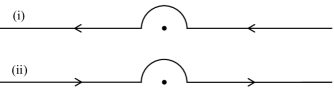
Figure 2: Contours of integration for (i) the ingoing and (ii) the outgoing particles.

In order to recover the Unruh temperature, we need to take into account the contribution from the time piece of the total action $S(t,\vec{x})=Et+S_{0}(\vec{x})$, as indicated by the formula of the temperature, (13), found in the previous section. The transformation of (6) into (7) indicates that the time coordinate has a discrete imaginary jump as one crosses the horizon at $x_{R^{\prime}}=-\frac{1}{2a}$, since the two time coordinate transformations are connected across the horizon by the change $t_{R^{\prime}}\rightarrow t_{R^{\prime}}-\frac{i\pi}{2a}$, that is,

$$\sinh(at_{R^{\prime}})\rightarrow\sinh\left(at_{R^{\prime}}-\frac{i\pi}{2}\right)=-i\cosh(at_{R^{\prime}})~{}.$$

Note that as the horizon is crossed, a factor of $i$ comes from the term in front of the hyperbolic function in (6), i.e.,

$$\sqrt{1+2ax_{R^{\prime}}}\rightarrow i\sqrt{|1+2ax_{R^{\prime}}|}~{},$$

so that (7) is recovered.

Therefore every time the horizon is crossed, the total action $S(t,\vec{x})=S_{0}(\vec{x})+Et$ picks up a factor of $E\Delta t=-\frac{i\pi E}{2a}$. For the temporal contribution, the direction in which the horizon is crossed does not affect the sign. This is different from the situation for the spatial contribution. When the horizon is crossed once, the total action $S(t,\vec{x})$ gets a contribution of $E\Delta t=-\frac{iE\pi}{2a}$, and for a round trip, as implied by the spatial part $\oint\;p_{x}dx$, the total contribution is $E\Delta t_{total}=-\frac{iE\pi}{a}$. So using the equation for the temperature (13) developed in the previous section, we obtain

$$T_{Unruh}=\frac{E\hbar}{\frac{\pi E}{a}+\frac{\pi E}{a}}=\frac{\hbar a}{2\pi}~{},$$ (19)

which is the Unruh temperature. The interesting feature of this result is that the gravitational WKB problem has contributions from both spatial and temporal parts of the wave function, whereas the ordinary quantum mechanical WKB problem has only a spatial contribution. This is natural since time in quantum mechanics is treated as a distinct parameter, separate in character from the spatial coordinates. However, in relativity time is on equal footing with the spatial coordinates.

V Conclusion

We have given a derivation of Unruh radiation in terms of the original heuristic explanation as tunneling of virtual particles tunneling through the horizon hawking . This tunneling method can easily be applied to different spacetimes and to different types of virtual particles. We chose the Rindler metric and Unruh radiation since, because of the local equivalence of acceleration and gravitational fields, it represents the prototype of all similar effects (e.g. Hawking radiation, Hawking–Gibbons radiation).

Since this derivation touches on many different areas – classical mechanics (through the H–J equations), relativity (via the Rindler metric), relativistic field theory (through the Klein–Gordon equation in curved backgrounds), quantum mechanics (via the WKB method for gravitational fields), thermodynamics (via the Boltzmann distribution to extract the temperature), and mathematical methods (via the contour integration to obtain the imaginary part of the action) – this single problem serves as a reminder of the connections between the different areas of physics.

This derivation also highlights several subtle points regarding the Rindler metric and the WKB tunneling method. In terms of the Rindler metric, we found that the different forms of the metric (3) and (5) do not cover the same parts of the full spacetime diagram. Also, as one crosses the horizon, there is an imaginary jump of the Rindler time coordinate as given by comparing (6) and (7).

In addition, for the gravitational WKB problem, $\Gamma$ has contributions from both the spatial and temporal parts of the action. Both these features are not found in the ordinary quantum mechanical WKB problem.

As a final comment, note that one can define an absorption probability (i.e., $P_{abs}\propto|\phi_{in}|^{2}$) and an emission probability (i.e., $P_{emit}\propto|\phi_{out}|^{2}$). These probabilities can also be used to obtain the temperature of the radiation via the “detailed balance method” padman

$$\frac{P_{emit}}{P_{abs}}=e^{-E/T}~{}.$$

Using the expression of the field $\phi=\phi_{0}e^{\frac{i}{\hbar}S(t,\vec{x})}$, the Schwarzschild–like form of the Rindler metric given in (5), and taking into account the spatial and temporal contributions gives an an absorption probability of

$$P_{abs}\propto e^{\frac{\pi E}{a}-\frac{\pi E}{a}}=1$$

and an emission probability of

$$P_{emit}\propto e^{-\frac{\pi E}{a}-\frac{\pi E}{a}}=e^{-\frac{2\pi E}{a}}~{}.$$

The first term in the exponents of the above probabilities corresponds to the spatial contribution of the action $S$, while the second term is the time piece. When using this method, we are not dealing with a directed line integral as in (9), so the spatial parts of the absorption and emission probability have opposite signs. In addition, the absorption probability is $1$, which physically makes sense – particles should be able to fall into the horizon with unit probability. If the time part were not included in $P_{abs}$, then for some given $E$ and $a$ one would have $P_{abs}\propto e^{\frac{\pi E}{a}}>1$, i.e., the probability of absorption would exceed $1$ for some energy. Thus for the detailed balance method the temporal piece is crucial to ensure that one has a physically reasonable absorption probability.

Acknowledgments

The authors would like to thank E.T. Akhmedov for valuable discussions. D.S. is supported by a 2008-2009 Fulbright Scholars Grant. D.S. would like to thank Vitaly Melnikov for the invitation to research at the Center for Gravitation and Fundamental Metrology and the Institute of Gravitation and Cosmology at PFUR. The authors would also like to thank two anonymous referees from this journal for their valuable comments and suggestions that led to the final version of this paper.

Appendix I: The Hamilton–Jacobi equations

The Hamilton–Jacobi equations may be derived from the Klein–Gordon equation in the following manner. The Klein–Gordon (KG) equation for a scalar field $\phi$ of mass $m$, placed in a background metric $g_{\mu\nu}$ is

$$\left(\frac{1}{\sqrt{-g}}\partial_{\mu}(\sqrt{-g}g^{\mu\nu}\partial_{\nu})-\frac{m^{2}c^{2}}{\hbar^{2}}\right)\phi=0~{},$$ (20)

where $c$ is the speed of light and $\hbar$ is Planck’s constant. For Minkowski spacetime, the above reduces to the free Klein–Gordon equation, i.e., $(\Box-m^{2}c^{2}/\hbar^{2})\phi=(-\partial^{2}/c^{2}\partial t^{2}+\nabla^{2}-m^{2}c^{2}/\hbar^{2})\phi=0$.

In using a scalar field, we are following the original works hawking ; unruh . Despite the fact that, absent the hypothetical Higgs boson, there are no known fundamental scalar fields, the derivation with spinor or vector particles would only add the complication of having to carry around spinor or Lorentz indices without adding to the basic understanding of the phenomenon. Using the WKB approach presented here it is straightforward to do the calculation using spinormann or vector particles.

Setting the speed of light $c$ equal to $1$, multiplying (20) by $-\hbar$ and using the product rule, (20) becomes

$$\begin{split}&\frac{-\hbar^{2}}{\sqrt{-g}}\Big{[}(\partial_{\mu}\sqrt{-g})g^{\mu\nu}\partial_{\nu}\phi+\sqrt{-g}(\partial_{\mu}g^{\mu\nu})\partial_{\nu}\phi+\\ &\sqrt{-g}g^{\mu\nu}\partial_{\mu}\partial_{\nu}\phi\Big{]}+m^{2}\phi=0~{}.\end{split}$$ (21)

The above equation can be simplified using the fact that the covariant derivative of any metric $g$ vanishes

$$\nabla_{\alpha}g^{\mu\nu}=\partial_{\alpha}g^{\mu\nu}+\Gamma^{\mu}_{\alpha\beta}g^{\beta\nu}+\Gamma^{\nu}_{\alpha\beta}g^{\mu\beta}=0~{},$$ (22)

where $\Gamma^{\mu}_{\alpha\beta}$ is the Christoffel connection. All the metrics that we consider here are diagonal so $\Gamma^{\mu}_{\alpha\beta}=0$, for $\mu\not=\alpha\not=\beta$. It can also be shown that

$$\Gamma^{\mu}_{\mu\gamma}=\partial_{\gamma}(\ln\sqrt{-g})=\frac{\partial_{\gamma}\sqrt{-g}}{\sqrt{-g}}~{}.$$ (23)

Using (22) and (23), the term $\partial_{\mu}g^{\mu\nu}$ in (21) can be rewritten as

$$\partial_{\mu}g^{\mu\nu}=-\Gamma^{\mu}_{\mu\gamma}g^{\gamma\nu}-\Gamma^{\nu}_{\mu\rho}g^{\mu\rho}=-\frac{\partial_{\gamma}\sqrt{-g}}{\sqrt{-g}}g^{\gamma\nu}~{},$$ (24)

since the harmonic condition is imposed on the metric $g^{\mu\nu}$, i.e., $\Gamma^{\nu}_{\mu\rho}g^{\mu\rho}=0$. Thus (21) becomes

$$-\hbar^{2}g^{\mu\nu}\partial_{\mu}\partial_{\nu}\phi+m^{2}\phi=0~{}.$$ (25)

We now express the scalar field $\phi$ in terms of its action $S=S(t,\vec{x})$

$$\phi=\phi_{0}e^{\frac{i}{\hbar}S(t,\vec{x})}~{},$$ (26)

where $\phi_{0}$ is an amplitude landau not relevant for calculating the tunneling rate. Plugging this expression for $\phi$ into (25), we get

$$-\hbar g^{\mu\nu}(\partial_{\mu}(\partial_{\nu}(iS)))+g^{\mu\nu}\partial_{\nu}(S)\partial_{\mu}(S)+m^{2}=0~{}.$$ (27)

Taking the classical limit, i.e., letting $\hbar\rightarrow 0$, we obtain the Hamilton–Jacobi equations for the action $S$ of the field $\phi$ in the gravitational background given by the metric $g_{\mu\nu}$,

$$g^{\mu\nu}\partial_{\nu}(S)\partial_{\mu}(S)+m^{2}=0~{}.$$ (28)

Appendix II: Hawking radiation from the Painlevé–Gulstrand form of the Schwarzschild spacetime

The Painlevé–Gulstrand form of the Schwarzschild spacetime is obtained by transforming the Schwarzschild time $t$ to the Painlevé–Gulstrand time $t^{\prime}$

$$dt=dt^{\prime}-\frac{\sqrt{\frac{2M}{r}}\,dr}{1-\frac{2\,M}{r}}.$$ (29)

Applying the above transformation to the Schwarzshild metric gives the Painlevé–Gulstrand form of the Schwarzschild spacetime

$$ds^{2}=-\left(1-\frac{2M}{r}\right)\,{dt^{\prime}}^{2}+2\sqrt{\frac{2M}{r}}\,dr\,dt^{\prime}+dr^{2}~{}.$$ (30)

The time is transformed, but all the other coordinates ($r,\theta,\phi$) are the same as the Schwarzschild coordinates. If we use the metric in (30) to calculate the spatial part of the action as in (35) and (16), we obtain

$$S_{0} = -\int_{-\infty}^{\infty}\frac{dr}{1-\frac{2M}{r}}\,\sqrt{\frac{2M}{r}}\,E$$ (31)

$$\pm \int_{-\infty}^{\infty}\frac{dr}{1-\frac{2M}{r}}\,\sqrt{E^{2}-m^{2}\left(1-\frac{2M}{r}\right)}.$$ (32)

Each of these two integrals has an imaginary contribution of equal magnitude, as can be seen by performing a contour integration. Thus one finds that for the ingoing particle (the $+$ sign in the second integral) one has a zero net imaginary contribution, while from for the outgoing particle (the $-$ sign in the second integral) there is a non–zero net imaginary contribution. Therefore in this case there is clearly a difference by a factor of two between using (9) and (10) which comes exactly because the tunneling rates from the spatial contributions in this case do depend upon the direction in which the barrier (i.e., the horizon) is crossed. The Schwarzcshild metric has a similar temporal contribution as for the Rindler metric akhmedov2 . The Painlevé–Gulstrand form of the Schwarzschild metric actually has two temporal contributions: (i) one coming from the jump in the Schwarzschild time coordinate similar to what occurs with the Rindler metric in (6) and (7); (ii) the second temporal contribution coming from the transformation between the Schwarzschild and Painlevé–Gulstrand time coordinates in (29). If one integrates equation (29), one can see that there is a pole coming from the second term. One needs to take into account both of these time contributions in addition to the spatial contribution, to recover the Hawking temperature. Only by adding the temporal contribution to the spatial part from (9), does one recover the Hawking temperature akhmedov2 $T=\frac{\hbar}{8\pi M}$. Thus for both reasons – canonical invariance and to recover the temperature – it is (9) which should be used over (10), when calculating $\Gamma_{QM}$. In ordinary quantum mechanics, there is never a case – as far as we know – where it makes a difference whether one uses (9) or (10). This feature – dependence of the tunneling rate on the direction in which the barrier is traverse – appears to be a unique feature of the gravitational WKB problem. So in terms of the WKB method as applied to the gravitational field, we have found that there are situations (e.g. Schwarzschild spacetime in Painlevé–Gulstrand coordinates) where the tunneling rate depends on the direction in which barrier is traversed so that (9) over (10) are not equivalent and will thus yield different tunneling rates, $\Gamma$.

Appendix III: Unruh radiation from the standard Rindler metric

For the standard form of the Rindler metric given by (3), the Hamilton–Jacobi equations become

$$-\frac{1}{(1+a\,x_{R})^{2}}\,(\partial_{t}S)^{2}+(\partial_{x}S)^{2}+m^{2}=0~{}.$$ (33)

After splitting up the action as $S(t,\vec{x})=Et+S_{0}(\vec{x})$, we get

$$-\frac{E}{(1+a\,x_{R})^{2}}\,+(\partial_{x}S_{0}(x_{R}))^{2}+m^{2}=0~{}.$$ (34)

The above yields the following solution for $S_{0}$

$$S^{\pm}_{0}=\pm\int_{-\infty}^{\infty}\frac{\sqrt{E^{2}-m^{2}\,(1+a\,x_{R})^{2}}}{1+a\,x_{R}}\,dx_{R}~{},$$ (35)

where the $+(-)$ sign corresponds to the ingoing (outgoing) particles.

Looking at (35), we see that the pole is now at $x_{R}=-1/a$ and a naive application of contour integration appears to give the results $\pm\frac{i\,\pi\,E}{a}$. However, this cannot be justified since the two forms of the Rindler metric – (3) and (5) – are related by the simple coordinate transformation (4), and one should not change the value of an integral by a change of variables. The resolution to this puzzle is that one needs to transform not only the integrand but the path of integration, so applying the transformation (4) to the semi–circular contour $x_{R^{\prime}}=-\frac{1}{2a}+\epsilon e^{i\theta}$ gives $x_{R}=-\frac{1}{a}+\frac{\sqrt{\epsilon}}{a}e^{i\theta/2}$. Because $e^{i\theta}$ is replaced by $e^{i\theta/2}$ due to the square root in the transformation (4), the semi–circular contour of (17) is replaced by a quarter–circle, which then leads to a contour integral of $i\frac{\pi}{2}\times{\rm Residue}$ instead of $i\pi\times{\rm Residue}$. Thus both forms of Rindler yield the same spatial contribution to the total imaginary part of the action.

References

- (1) S.W. Hawking, “Particle creation by black holes,” Comm. Math. Phys. 43, 199-220 (1975).
- (2) G.W. Gibbons and S.W Hawking, “Cosmological event horizons, thermodynamics, and particle creation,” Phys. Rev. D 15, 2738-2751 (1977).
- (3) W.G. Unruh, “Notes on black hole evaporation,” Phys. Rev. D 14, 870-892 (1976).
- (4) P. Kraus and F. Wilczek, “Effect of self-interaction on charged black hole radiance,” Nucl. Phys. B 437 231-242 (1995); E. Keski-Vakkuri and P. Kraus, “Microcanonical D-branes and back reaction,” Nucl. Phys. B 491 249-262 (1997).
- (5) K. Srinivasan and T. Padmanabhan, “Particle production and complex path analysis,” Phys. Rev. D 60 024007 (1999); S. Shankaranarayanan, T. Padmanabhan and K. Srinivasan, “Hawking radiation in different coordinate settings: complex paths approach,” Class. Quant. Grav. 19, 2671-2688 (2002).
- (6) M.K. Parikh and F. Wilczek, “Hawking radiation as tunneling,” Phys. Rev. Lett. 85, 5042-5045 (2000).
- (7) M.K. Parikh, “A secret tunnel through the horizon,” Int. J. Mod. Phys. D 13, 2351-2354 (2004).
- (8) Y. Sekiwa, “Decay of the cosmological constant by Hawking radiation as quantum tunneling”, arXiv:0802.3266
- (9) G.E. Volovik, “On de Sitter radiation via quantum tunneling,” arXiv:0803.3367 [gr-qc]
- (10) A.J.M. Medved, “A Brief Editorial on de Sitter Radiation via Tunneling,” arXiv:0802.3796 [hep-th]
- (11) V. Akhmedova, T. Pilling, A. de Gill and D. Singleton, “Temporal contribution to gravitational WKB-like calculations,” Phys. Lett. B 666 269-271 (2008). arXiv:0804.2289 [hep-th]
- (12) Qing-Quan Jiang, Shuang-Qing Wu, and Xu Cai, “Hawking radiation as tunneling from the Kerr and Kerr-Newman black holes,” Phys. Rev. D 73, 064003 (2006) [hep-th/0512351]
- (13) Jingyi Zhang, and Zheng Zhao, “Charged particles tunneling from the Kerr-Newman black hole,” Phys. Lett. B 638, 110-113 (2006) [gr-qc/0512153]
- (14) V. Akhmedova, T. Pilling, A. de Gill, and D. Singleton, “Comments on anomaly versus WKB/tunneling methods for calculating Unruh radiation,” Phys. Lett. B 673, 227-231 (2009). arXiv:0808.3413 [hep-th]
- (15) R. Kerner and R. B. Mann, “Fermions tunnelling from black holes,” Class. Quant. Grav. 25, 095014 (2008). arXiv:0710.0612
- (16) A.J.M. Medved and E. C. Vagenas, “On Hawking radiation as tunneling with back-reaction” Mod. Phys. Lett. A 20, 2449-2454 (2005) [gr-qc/0504113]; A.J.M. Medved and E. C. Vagenas, “On Hawking radiation as tunneling with logarithmic corrections”, Mod. Phys. Lett. A 20, 1723-1728 (2005) [gr-qc/0505015]
- (17) J.F. Donoghue and B.R. Holstein, “Temperature measured by a uniformly accelerated observer”, Am. J. Phys. 52, 730-734 (1984).
- (18) J.D. Jackson “On understanding spin-flip synchrotron radiation and the transverse polarization of electrons in storage rings” Rev. Mod. Phys. 48, 417-433 (1976)
- (19) J.S. Bell and J.M. Leinaas, “Electrons As Accelerated Thermometers” Nucl. Phys. B 212, 131-150 (1983); J.S. Bell and J.M. Leinaas, “The Unruh Effect And Quantum Fluctuations Of Electrons In Storage Rings” Nucl. Phys. B 284, 488-508 (1987)
- (20) E. T. Akhmedov and D. Singleton, “On the relation between Unruh and Sokolov-Ternov effects”, Int. J. Mod. Phys. A 22, 4797-4823 (2007). hep-ph/0610391; E. T. Akhmedov and D. Singleton, “On the physical meaning of the Unruh effect”, JETP Phys. Letts. 86, 615-619 (2007). arXiv:0705.2525 [hep-th]
- (21) A. Retzker, J.I. Cirac, M.B. Plenio, and B. Reznik, Phys. Rev. Lett. 101, 110402 (2008).
- (22) C. W. Misner, K. S. Thorne and J. A. Wheeler, Gravitation, W. H. Freeman and Company, San Francisco, 1973
- (23) P.M. Alsing and P.W. Milonni, “Simplified derivation of the Hawking-Unruh temperature for an accelerated observer in vacuum,” Am. J. Phys. 72, 1524-1529 (2004). quant-ph/0401170
- (24) E. F. Taylor and J. A. Wheeler, Spacetime Physics, Freeman, San Francisco, 1966.
- (25) N. D. Birrell and P. C. W. Davies, Quantum Fields in Curved Space, Cambridge University Press, New York, 1982.
- (26) M. Visser, Lorentzian Wormholes: from Einstein to Hawking, AIP Press, New York, 1995.
- (27) L.P. Grishchuk, Y.B. Zeldovich and L.V. Rozhansky, “Equivalence principle and zero point field fluctuations,” Sov. Phys. JETP 65, 11 (1987) [Zh. Eksp. Teor. Fiz. 92, 20 (1987)].
- (28) L. D. Landau and E. M. Lifshitz, Quantum Mechanics: Non-Relativistic Theory, (Vol. 3 of Course of Theoretical Physics), 3rd ed., Pergamon Press, New York, 1977.
- (29) D. J. Griffiths, Introduction to Quantum Mechanics, 2nd ed., Pearson Prentice Hall, Upper Saddle River, NJ, 2005.
- (30) J. Schwinger, “On Gauge Invariance and Vacuum Polarization”, Phys. Rev. 82, 664-679 (1951).
- (31) B.R. Holstein, “Strong field pair production”, Am. J. Phys. 67, 499-507 (1999).
- (32) B. D. Chowdhury, “Problems with tunneling of thin shells from black holes,” Pramana 70, 593-612 (2008). hep-th/0605197
- (33) E.T. Akhmedov, V. Akhmedova, and D. Singleton, “Hawking temperature in the tunneling picture,” Phys. Lett. B 642, 124-128 (2006). hep-th/0608098
- (34) E.T. Akhmedov, V. Akhmedova, T. Pilling, and D. Singleton, “ Thermal radiation of various gravitational backgrounds,” Int. J. Mod. Phys. A 22, 1705-1715 (2007). hep-th/0605137
- (35) R. Banerjee and B.R. Majhi, “Hawking black body spectrum from tunneling mechanism,” Phys. Lett. B 675, 243-245 (2009)
- (36) E.T. Akhmedov, T. Pilling, D. Singleton, “Subtleties in the quasi-classical calculation of Hawking radiation,” Int. J. Mod. Phys. D, 17 2453-2458 (2008). GRF “Honorable mention” essay, arXiv:0805.2653 [gr-qc]