Disentangling the metallicity and star formation history of HII galaxies through tailor-made models

Abstract

We present a self-consistent study of the stellar populations and the ionized gas in a sample of 10 HII galaxies with, at least, four measured electron temperatures and a precise determination of ionic abundances following the ”direct method”. We fitted the spectral energy distribution of the galaxies using the program STARLIGHT and Starburst99 libraries in order to quantify the contribution of the underlying stellar population to the equivalent width of H$\beta$ (EW(H$\beta$)), which amounts to about 10 % for most of the objects. We then studied the Wolf-Rayet stellar populations detected in seven of the galaxies. The presence of these populations and the EW(H$\beta$) values, once corrected for the continuum contribution from underlying stars and UV dust absorption, indicate that the ionizing stellar populations were created following a continuous star formation episode of 10 Myr duration, hence WR stars may be present in all of objects even if they are not detected in some of them.

The derived stellar features, the number of ionizing photons and the relative intensities of the most prominent emission lines were used as input parameters to compute tailored models with the photoionization code CLOUDY. Our models are able to adequately reproduce the thermal and ionization structure of these galaxies as deduced from their collisionally excited emission lines. This indicates that ionic abundances can be derived following the ”direct method” if the thermal structure of the ionized gas is well traced, hence no abundance discrepancy factors are implied for this kind of objects. Only the electron temperature of S⁺ is overestimated by the models, with the corresponding underestimate of its abundance, pointing to the possible presence of outer shells of diffuse gas in these objects that have not been taken into account in our models. This kind of geometrical effects can affect the determination of the equivalent effective temperature of the ionizing cluster using calibrators which depend on low-excitation emission lines.

1 Introduction

The understanding of the physical properties of gas, stars, and dust and their interrelations and evolution in different scenarios of star formation constitute one of the most intriguing open issues on astrophysics. This type of phenomenon is well studied at different spatial scales, since massive young star clusters are powerful sources of radiation, detectable even in the most distant galaxies. For instance, from a statistical point of view, large surveys of starburst galaxies have been used to confirm, with a great confidence base, some of the observational relations between the physical properties of different types of galaxies at different cosmological epochs. This is the case of the luminosity-metallicity relation or its equivalent, the mass-metallicity relation, which establishes that in the local Universe the most massive galaxies have, in average, higher metallicities than the less massive ones (SDSS: Tremonti et al., 2004; 2dFGRS: Lamareille et al., 2004). This observational fact is a consequence of higher stellar yields in the more massive galaxies, which could find less troubles to retain the metals ejected by stars and pushed out towards the interstellar and intergalactic medium by supernovae and stellar winds (Larson, 1974).

Nevertheless, since this kind of studies are mostly based on the relation between the stellar mass and the oxygen gas-phase abundance, they present some drawbacks, involving several aspects in the determination of their properties, including the following: 1) The relation between the total mass of a galaxy and its stellar mass depends strongly on different environmental and morphological circumstances (Bell & de Jong, 2001). 2) The stellar mass is usually estimated by means of stellar synthesis population model fitting of the spectral energy distribution (SED). These models are often affected by degeneracies between age, metallicity, and dust-extinction which are never well solved (Renzini & Buzzoni, 1986). 3) The metallicity is only estimated in starburst galaxies through the oxygen gas phase abundance derived from the relative intensities of the most prominent emission lines. This excludes from these studies the most quiescent and early-type galaxies. 4) The spatial distribution of metallicity in massive, non-compact objects is often neglected, assigning a unique value to the whole distribution. However, it is known that the radial profile of the oxygen abundance in some close spiral galaxies can spread over more than an order of magnitude (Searle, 1971). 5) The strong-line parameters used to derive metallicities are often calibrated employing sequences of models which do not follow the distribution of metallicity obtained with more confident observational methods like, for instance, the direct method (Pérez-Montero & Díaz, 2005), which is based on the previous determination of the electron temperature of the ionized gas by means of the fainter auroral emission lines.

HII galaxies usually represent the low-end of the mass-metallicity relation in different surveys. In fact, the work of Lequeux et al. (1979), the first where the correlation between oxygen gas phase abundance and stellar mass was found, is based on this type of blue dwarf irregular galaxies. Their spectra are characterized by very bright emission lines while the total luminosity and color are dominated by the presence of intense bursts of recent star formation (Sargent & Searle, 1970; French, 1980). They are dwarf and compact so they seldom show chemical inhomogeneities. The metallicity distribution of HII galaxies has an average value (12+log(O/H) $\sim$ 8.0, Terlevich et al., 1991) sensibly lower than the rest of starburst galaxies and, in fact, the objects with the lowest metal content in the Local Universe belong to the subclass of HII galaxies (IZw18, Searle & Sargent, 1972).

Sloan Digital Sky Survey (SDSS) represents the largest sample of galaxies in the Local Universe and it has been explored for the study of the mass-metallicity relation (Tremonti et al., 2004). Unfortunately, this survey presents some drawbacks that prevent a precise determination of the metallicity in the emission lines-like objects: 1) Since the spectral coverage of the survey starts at 3800 Å, the sample objects at redshift $\sim$ 0 have not any detection of the [Oii] $\lambda$ 3727 Å line and hence no direct measurement of the total abundance of oxygen is possible. Only an estimate can be given in terms of the weaker auroral lines at $\lambda\lambda$ 7319,7330 Å but with a high degree of uncertainty (Kniazev et al., 2003). 2) Only a fraction of the objects show in their spectra the weak auroral emission lines necessary to estimate the electron temperature and, hence, to calculate chemical abundances following the direct method (Izotov et al., 2006). 3) The only auroral lines seen in the most part of this subsample is [Oiii] $\lambda$ 4363 Å and, therefore, only the electron temperature of the high excitation zone can be derived. The total ionization structure of the nebula is then often obtained based on this temperature through a very simplified assumption (Pérez-Montero & Díaz, 2003). 4) For the rest of the objects with no direct electron temperature derivation, a strong-line method is used, so the determination of metallicity is hugely sensitive to the chosen calibration (Kewley & Ellison, 2008). 5) The 3 arc secs aperture of the SDSS fiber precludes a good determination of the physical properties of the starburst region of these galaxies.

Double-arm spectrographs are suitable tools to observe the entire spectral range between 3500 Å and 1 micron in one single exposure at good spectral resolution the star forming regions of HII galaxies, avoiding the effects due to a different covering of the object in different spectral ranges. In the case of compact HII galaxies, their bursts of star formation can be covered entirely with a narrow slit. Assuming that different electron temperatures are measured in the optical spectrum, this implies that different excitation regions inside the ionized gas can be characterized, leading to a more precise determination of the ionic chemical abundances. There are some reported discrepancies between abundance determinations obtained from bright collisional lines and the fainter recombination ones (Peimbert et al., 2007), which do not depend on the determination of the electron temperature. Nevertheless, the existence of these abundance discrepancy factors (ADFs) is still not conclusively established. In fact, in the case of HII galaxies, no significant deviations have been found between the electron temperatures derived from collisional lines and from the Balmer (Hägele et al., 2006) or Paschen discontinuities (Guseva et al., 2006). Besides, the high ADFs derived from optical recombination lines are sensibly lower than those calculated from mid-infra-red lines (Wu et al., 2008; Lebouteiller et al., 2008) or from planetary nebulae (Williams et al., 2008 ).

Table 1: List of the modeled objects, with some additional basic information.

Object ID	hereafter ID	Publication	redshift	log L(H$\alpha$)	12+log(O/H)	Other names
		(Telescope)		(erg $\cdot$ s-1)
SDSS J002101.03+005248.1	J0021	H06 (WHT)	0.098	42.13	8.10 $\pm$ 0.04	UM228, SHOC 11
SDSS J003218.60+150014.2	J0032	H06 (WHT)	0.018	40.30	7.93 $\pm$ 0.03	SHOC 22
SDSS J145506.06+380816.6	J1455	H08 (CAHA - 3.5 m.)	0.028	40.84	7.94 $\pm$ 0.03	CG 576
SDSS J150909.03+454308.8	J1509	H08 (CAHA - 3.5 m.)	0.048	41.26	8.19 $\pm$ 0.03	CG 642
SDSS J152817.18+395650.4	J1528	H08 (CAHA - 3.5 m.)	0.064	41.63	8.17 $\pm$ 0.04
SDSS J154054.31+565138.9	J1540	H08 (CAHA - 3.5 m.)	0.011	39.65	8.07 $\pm$ 0.05	SHOC 513
SDSS J161623.53+470202.3	J1616	H08 (CAHA - 3.5 m.)	0.002	38.93	8.01 $\pm$ 0.03
SDSS J162410.11-002202.5	J1624	H06 (WHT)	0.031	41.48	8.05 $\pm$ 0.02	SHOC 536
SDSS J165712.75+321141.4	J1657	H08 (CAHA - 3.5 m.)	0.038	40.74	7.99 $\pm$ 0.04
SDSS J172906.56+565319.4	J1729	H08 (CAHA - 3.5 m.)	0.016	40.57	8.08 $\pm$ 0.04	SHOC 575

In this work we model the stellar content and the abundances of the most representative ions of a sample of HII galaxies previously observed in the SDSS and re-observed with different double arm spectrographs in the spectral range between 3500 Å and 1 micron (Hägele et al., 2006, hereafter H06 and Hägele et al., 2008, hereafter H08). The study of the stellar population in the star forming knots of these galaxies includes underlying and ionizing populations. We show that the correct characterization of the ionizing stellar population, including Wolf-Rayet stars, and an appropriate geometry of the gas, dust content and the abundances of the main elements are enough to reproduce with precision the intensities of the observed emission lines. We demonstrate too that it is possible to draw a consistent picture of the thermal and ionization structure of the gas based on the measurement of as many electron temperatures as possible and, hence, to calculate ionic abundances with high precision using optical to far red collisional emission lines.

In the next section we describe the sample of objects that we have modeled. In section 3 we describe our results concerning the stellar content through model fitting of the SED and the analysis of the Wolf-Rayet features. We also describe the photoionization models of the gas, once the underlying stellar population has been removed. In section 4, we discuss the star formation history and the physical properties obtained from the models and we compare them with observations. In section 5, we summarize our results and present our conclusions. Finally, an appendix has been added to compare the total abundances and ionization correction factors obtained from models with those obtained in H06 and H08.

2 The sample of studied objects

The modeled galaxies were selected from the SDSS using the implementation of the database in the INAOE Virtual Observatory superserver (see H06 and H08 for more details) . We selected the brightest nearby narrow emission line galaxies with very strong lines and large equivalent widths of the H$\alpha$ line from the whole SDSS data release available when we planned each observing run. Once AGN-like objects were removed by BPT diagnostic diagrams (Baldwin, Phillips and Terlevich, 1981), the sample was restricted to the largest H$\alpha$ flux and highest signal-to-noise ratio objects (López, 2005). The HII galaxies studied in this work comprise 10 objects belonging to the final list and observed in two independent observing runs with different double-arm spectrographs in order to improve the spectral range and the signal-to-noise. Three out of them were observed with the ISIS spectrograph mounted on the William Herschel Telescope (H06) and the other 7 were observed with the TWIN instrument in the 3.5 m. CAHA telescope (H08). In Table 1 we list the galaxies, with the names adopted in this work, the spectroscopic redshift as listed in the SDSS catalogue and their extinction-corrected H$\alpha$ luminosities in erg$\cdot$s^-1. Distances have been derived from the measured redshifts for cosmological parameters: H₀ = 73 km s^-1 Mpc^-1, $\Omega_{matter}$ = 0.27, $\Omega_{vaccum}$ = 0.73. We also list the oxygen abundance as calculated in H06 and H08 and, finally, other names by which the galaxies are also known.

Both observing runs had similar configurations. In WHT observations the spectral range goes from 3200 Å up to 10550 Å with a spectral dispersion of 2.5 Å/px FWHM in the blue arm and 4.8 in the red. In CAHA observations, the spectral range covers from 3400 up to 10400 Å (with a gap between 5700 and 5800 Å) with spectral resolutions of 3.2 and 7.0 Å/px FWHM in the blue and the red part respectively. The observations were taken at parallactic angle. These configurations allow to detect simultaneously the bright emission lines from [Oii] at 3727 Å up to [Siii] at 9532 Å, allowing the derivation of five different electron temperatures (t([Oii]), t([Oiii]), t([Sii]), t([Siii]) and t([Nii]) ) in three objects of the sample and four temperatures (the same listed above with the exception of t([Nii]) in the other seven). The derivation of all these electron temperatures allows a more precise determination of the thermal structure of the gas and, hence, of the ionic abundances of the detected species in the observed spectra. Our sample galaxies have oxygen abundances in the range 7.93 $<$ 12+log(O/H) $<$ 8.19 and equivalent widths of H$\beta$ in the range 83 Å $<$ EW(H$\beta$) $<$ 171 Å.

3 Results

3.1 Model fitting of the stellar population

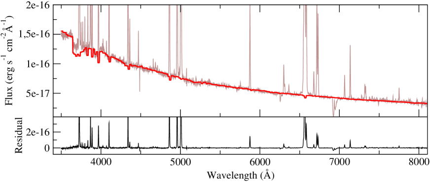
Figure 1: In the solid brown line, optical spectrum of the galaxy J0021 and comparison with the spectral fitting carried out with the code STARLIGHT, using spectral libraries from Starburst99, represented by the solid red line. In the lower panel, we show the residuals of the fit, which represents the nebular spectrum.

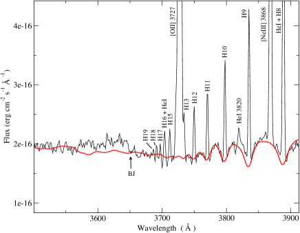
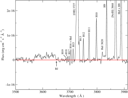
Figure 2: Upper panel, in black, optical spectrum of the galaxy J1624 in the spectral range 3500 - 3912 Å, around the Balmer jump and the high order Balmer series, together with the fitting (red line) performed using the STARLIGHT spectral synthesis code. Lower panel, subtraction of this fitting from the WHT spectrum in the same spectral range; the solid red line shows the zero level.

Underlying stellar populations in starburst galaxies have several effects in their spectra that can affect the measurement of emission lines. Firstly, since this population has a weight in the galaxy continuum, most of the times the measurement of the equivalent widths of the emission lines is not a trustable estimator of the age of the ionizing stellar population (Terlevich et al., 2004). Secondly, the presence of a conspicuous underlying stellar population depresses the Balmer and Paschen emission lines and do not allow to measure their fluxes with an acceptable accuracy (Díaz, 1988). This can alter those properties dependent on the fluxes of these recombination lines, like the reddening or the ionic abundances. In the case of the helium recombination lines, this effect is present too, affecting the derivation of the helium abundance (Olive & Skillman, 2004).

We have subtracted from the observed spectra the spectral energy distribution of the underlying stellar population found by the spectral synthesis code STARLIGHT (Cid Fernandes et al. 2004, 2005; Mateus et al. 2005). STARLIGHT fits an observed continuum spectral energy distribution using a combination of multiple simple stellar population synthetic spectra (SSPs; also known as instantaneous burst) using a $\chi^{2}$ minimization procedure. In order to keep the consistency with the photoionization models used to model the gas emission, we have chosen for our analysis the SSP spectra from the Starburst99 libraries (Leitherer et al., 1999; Vázquez & Leitherer, 2005), based on stellar model atmospheres from Smith et al. (2002), Geneva evolutionary tracks with high stellar mass loss (Meynet et al., 2004), a Kroupa Initial Mass Function (IMF; Kroupa, 2002) in two intervals (0.1-0.5 and 0.5-100 M_⊙) with different exponents (1.3 and 2.3 respectively), the theoretical wind model (Leitherer et al., 1992) and a supernova cut-off of 8 M_⊙. We have fixed the metallicity of the stellar populations to Z = 0.004 (= 1/5 Z_⊙) and Z = 0.008 (= 2/5 Z_⊙) depending on the closest total oxygen abundance as measured using the direct method for each galaxy ( see H06 and H08). The STARLIGHT code solves simultaneously the ages and relative contributions of the different SSPs and the average reddening. The reddening law from Cardelli, Clayton & Matthews (1989) has been used. Prior to the fitting procedure, the spectra were shifted to the rest-frame, and re-sampled to a wavelength interval of 1 Å in the entire wavelength range between 3500 Å and 9000 Å by interpolation conserving flux, as required by the program. Bad pixels and emission lines were excluded from the final fits.

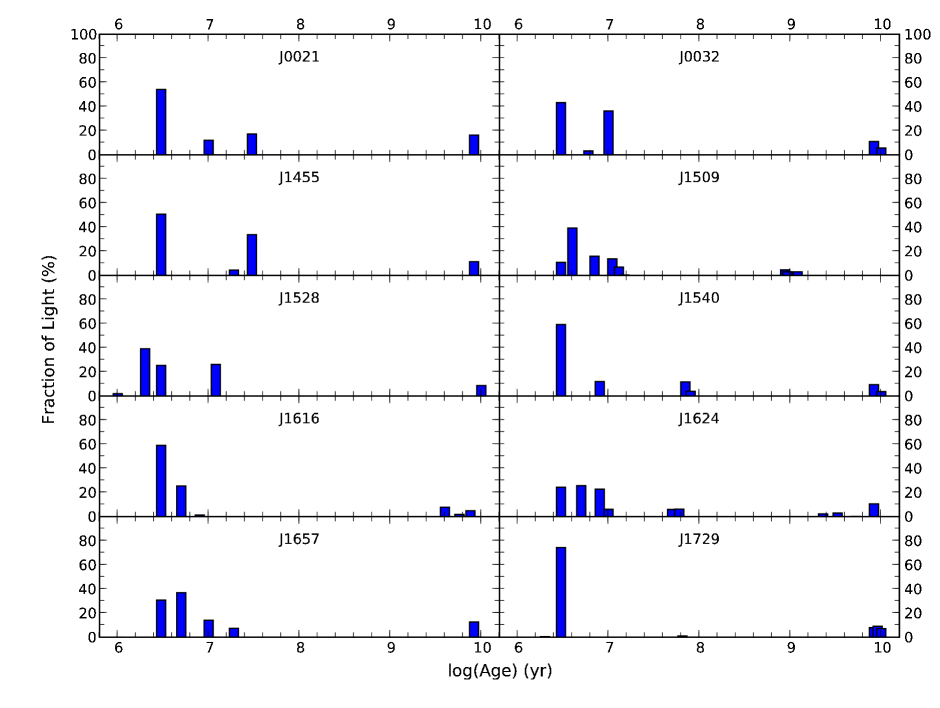
Figure 3: Histogram of the distribution of the percentage of visual light from each population in the best solution found by STARLIGHT in the spectral fitting of the optical spectrum for each galaxy of the sample.

To illustrate the fitting results, we show in the upper panel of Figure 1 the spectrum of J0021 with the best fit found by STARLIGHT overimposed and, in the lower panel of the same figure, the emission line spectrum once the underlying stellar continuum has been subtracted. The measured intensities of the most prominent Balmer emission lines in this subtracted spectrum are, in all cases, equal within the errors to those reported in H06 and H08, where a pseudo-continuum was adopted. It was also shown in those works that the measurement of the intensities of the Balmer lines is consistent with a multi-gaussian fitting of the lines. This method fits independently the emission line and the absorption feature, which is visible through their wings in some bright Balmer lines. In the upper panel of Figure 2 we plot in detail the WHT spectrum of J1624 in the spectral range 3500-3912 Å, around the Balmer jump and the high order Balmer series, and in solid red line we show the STARLIGHT fitting. In the lower panel of the same figure we show the subtraction of the fit from the observed spectrum. We can appreciate that small errors in the fit of the underlying stellar population could become a great unquantifiable error in the emission line fluxes. Nevertheless, for the strongest emission lines, the differences between the measurements done after the subtraction of the STARLIGHT fit and those using the pseudo-continuum approximation are well below the observational errors, giving almost the same result. It must be highlighted that in this type of objects the absorption lines, used to fit the underlying stellar populations, are mostly affected by the presence of emission lines. There are a few that are not, such as some calcium and magnesium absorption lines. To make the STARLIGHT fit it is necessary to mask the contaminated lines, thus the fit is based on the continuum shape and takes into account only a few absorption lines. Hence, it is not surprising that the STARLIGHT results are not so good for this kind of objects. It must be noted too that the STARLIGHT methodology is very advantageous for statistical and comparative studies. Those studies only consider the results derived from the strongest emission lines which have small proportional errors. However, we must be careful when the aim of our work is the detailed and precise study of a reduced sample of objects because, as we have shown, we can not quantify the error introduced by the fitting. Moreover, these errors are higher for the weakest lines, including the auroral ones. Regarding helium absorption features the multigaussian approximation is not possible in any line, because their wings are not visible. Nevertheless, we have checked that the contribution of the depressed components of the emission lines predicted by the STARLIGHT fit are not larger than taking into account a slightly lower position of the continuum, as it is explained in both H06 and H08.

¿From this analysis we only take as a valuable input information for our tailor-made photoionization models, the ratios predicted by STARLIGHT for the ionizing and the underlying stellar populations in order to correct the equivalent width of H$\beta$ and to take it as an estimate of the properties of the ionizing stellar population.

Table 2: Properties of the stellar populations as obtained with STARLIGHT for each studied object. In the last two columns we list the measured EW(H$\beta$) and its value corrected for contribution to the continuum from the young stellar component only.

Object ID	A(V)	log M∗	log Mion∗	% Mion∗	EW(H$\beta$) obs.	EW(H$\beta$)$cor$
	(mag)	(M⊙)	(M⊙)		(Å)	(Å)
J0021	0.01	9.40	6.89	0.31	97	110
J0032	0.17	8.15	5.53	0.24	90	119
J1455	0.09	8.42	6.04	0.42	133	146
J1509	0.58	8.08	6.96	7.57	123	135
J1528	0.25	8.92	6.81	0.78	171	191
J1540	0.42	7.51	5.22	0.52	122	124
J1616	-0.11	6.55	4.50	0.89	83	83
J1624	0.60	8.88	5.73	0.07	101	107
J1657	0.16	8.45	6.20	0.56	118	132
J1729	0.27	8.65	6.07	0.26	126	126

Nevertheless, we can do a comparative analysis of the star formation histories of every galaxy as predicted by the population synthesis fitting technique. In Figure 3, we show the histogram of the age distribution of the contribution to the visual light of each stellar population used by STARLIGHT to fit the optical SED for the ten studied galaxies As we can see, the blue light in these objects seems to be largely dominated by a very young stellar population (younger than 10 Myr) which is responsible for the ionization of the gas. At same time, there are different underlying stellar populations, with a component older than 1 Gyr in all cases. This ”old” component dominates the total stellar mass in all the objects, providing more than 99 % of it, with the exception of J1509, for which this percentage is about 92 %. At any rate, we find very similar age distributions for the stellar populations in all the objects pointing to very similar star formation histories with the presence of recursive starburst episodes resembling the one observed at present.

In table 2, we summarize the properties of the best fitting to the optical spectrum of each galaxy as found by STARLIGHT. We list in columns 2 to 5 the visual extinction, A(V), the total stellar mass, M_∗, the mass of the stellar population younger than 10 Myr, M_ion∗, and the percentage contribution of this to the total stellar mass, % M_ion∗. We also list in columns 6 and 7 the measured equivalent width of H$\beta$, EW(H$\beta$), and the corrected value, once the contribution to the continuum by the underlying stellar population has been subtracted. As we can see, our procedure yields a negative value for the extinction in J1616. Nevertheless, this is still consistent with the very low extinction found using the Balmer decrements.

We can check the accuracy of these fittings by comparing the stellar mass of the ionizing population as derived from STARLIGHT, and the values of the same masses as derived from the extinction-corrected H$\alpha$ fluxes, using the expression from Díaz (1998):

$$\log M_{ion*}=\log L(H\alpha)-0.86\cdot\log EW(H\beta)-32.61$$ (1)

This comparison is shown in Figure 4. It can be seen that the agreement between both derived values is very good for most of the studied objects. Only J0021 shows a higher young stellar mass when derived from its H$\alpha$ flux. Horizontal error bars in the plot correspond to the underestimate of the H$\alpha$ flux due to the UV dust absorption. We have quantified this effect taking the absorption factors derived from the photoionization models described in section 3.3 below. Nevertheless, taking into account these corrected values of L(H$\alpha$) in the derivation of M_ion∗ from (1) does not increase the ionizing stellar masses by more than 0.3 dex, except in the case of J1455, with 0.42 dex.

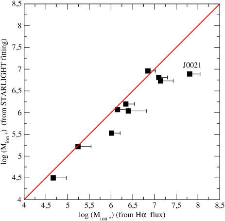
Figure 4: Comparison between the ionizing stellar mass as derived from the extinction-corrected H$\alpha$ fluxes and from SED fitting for an age younger than 10 million years. The red solid line represents the 1:1 relation. Error bars to the right take into account the dust absorption factors obtained from the photoionization models described below.

3.2 Detection and measurement of Wolf-Rayet bumps

Table 3: Observed extinction corrected H$\beta$ intensities and properties of the WR bumps for the objects of the sample. We list equivalent widths and relative intensities, normalized to 100 times the H$\beta$ value, measured at 4650 Å (blue bump, bb) and at 5808 Å (red bump, rb). The corrected values take into account the contribution of the underlying stellar population and the nebular emission to the continuum and the dust absorption of the UV predicted by the photoionization models in each object.

Object ID	I(H$\beta$)	-EW(bb)	-EW(bb)cor	I(bb)	I(bb)${}_{cor}^{a}$	-EW(rb)	-EW(rb)cor	I(rb)a	I(rb)${}_{cor}^{a}$
	(erg $\cdot$ s-1 cm-2)	(Å)	(Å)			(Å)	(Å)
J0021	2.47 $\cdot$ 10-14	3.9$\pm$0.9	5.8	1.4$\pm$0.3	0.8	–	–	–	–
J0032	1.23 $\cdot$ 10-14	5.1$\pm$1.0	6.7	4.9$\pm$1.0	3.2	1.3$\pm$0.6	1.9	0.9$\pm$0.4	0.6
J1455	1.49 $\cdot$ 10-14	–	–	–	–	–	–	–	–
J1509	1.35 $\cdot$ 10-14	9.1$\pm$2.0	12.0	8.3$\pm$1.8	5.3	1.6$\pm$0.5	2.2	1.1$\pm$0.4	0.7
J1528	1.73 $\cdot$ 10-14	–	–	–	–	–	–	–	–
J1540	5.30 $\cdot$ 10-15	10.3$\pm$2.8	16.5	9.8$\pm$2.6	9.5	–	–	–	–
J1616	1.36 $\cdot$ 10-14	5.5$\pm$3.8	6.6	6.9$\pm$4.8	3.3	–	–	–	–
J1624	5.03 $\cdot$ 10-14	7.4$\pm$1.5	13.1	2.6$\pm$0.6	1.3	2.8$\pm$0.9	3.8	0.8$\pm$0.3	0.4
J1657	6.30 $\cdot$ 10-15	–	–	–	–	–	–	–	–
J1729	2.40 $\cdot$ 10-14	6.5$\pm$2.1	9.4	6.5$\pm$2.1	3.4	–	–	–	–

Wolf-Rayet (WR) stars appear in the first stages after the main sequence phase of the evolution of massive stars, so they are already visible soon after the beggining of a burst of star formation (approximately 2 Myr) and for a relatively short period of time (about 3 Myr, on average). The existence of this WR stellar population can be very useful for the study and characterization of the ionizing stellar population in starburst galaxies (e.g. Pérez-Montero & Díaz, 2007). The strength of the stellar winds produced by these stars can be sometimes measured in the integrated spectra of the starburst galaxies, which are then identified as WR galaxies (Conti, 1991). The presence of the emission broad features (”bumps”) produced by WR stars are therefore associated to the existence of processes of intense star formation. These WR features are the blue bump, centered at 4650 Å and produced mainly by broad emission lines of Nv at 4605, 4620 Å, Niii 4634, 4640 Å, Ciii/iv 4650, 4658 Å and Heii at 4686 Å, and the red bump, usually fainter, centered at 5808 Å and emitted mainly by Ciii.

We have detected the blue bump in seven of the ten galaxies of our sample, while the red bump has been detected in only three of these seven galaxies. All the three galaxies observed with WHT had already been identified as WR galaxies in H06 and have also been included in the catalogue of WR galaxies of the SDSS (Brinchmann et al., 2008). The other four galaxies with a detection of WR features, observed with the 3.5 CAHA telescope are not listed in that catalogue. An example of the WR emission can be seen in Figure 6 of H06 for the J1624 galaxy.

We have measured the bumps in the following way. First we have adopted a continuum shape and we have measured the broad emission over this continuum at the wavelengths of the blue bump, at 4650 Å, and the red bump, at 5808 Å. Finally, we have subtracted the emission of the narrower lines not emitted by the WR stars winds, which are [Feiii] 4658 Å, the narrow component of Heii 4686 Å, Hei + [Ariv] 4711 Å and [Ariv] 4740 Å in the blue bump. The equivalent widths and the deredenned relative intensities of the blue and red bumps are shown in Table 3. Both have been corrected in order to study the properties of the ionizing stellar population. In the case of EWs, we have subtracted the contribution of the underlying stellar population as derived from STARLIGHT and from the nebular continuum as derived from the photoionization models described below. In the case of the relative intensities, we have taken into account the dust absorbed component of H$\beta$ derived from the same photoionization models for each object.

3.3 Photoionization models of the ionized gas

Photoionization models have been calculated using the code CLOUDY v. 06.02c (Ferland et al., 1998) with the same atomic coefficients used to derive ionic abundances in H06 and H08 and the recent dielectronic recombination rate coefficients from Badnell (2006). We have taken the same Starburst99 stellar libraries used by STARLIGHT to fit the observed SEDs. We have assumed different initial input parameters and then, we have followed an iterative method to fit the relative intensities of the strongest emission lines in the integrated spectra, along with other observable properties.

We have assumed a constant star formation history, with a star formation rate calculated according to the measured and corrected number of ionizing photons. The age of this burst of star formation has been limited to the range 1-10 Myr in order to reproduce the corrected equivalent width of H$\beta$ once the older stellar populations have been removed, except in the case of J1540 for which a burst duration of 15.85 Myr has been considered in order to reproduce the observed EW(H$\beta$). Total abundances have been set to match the values derived in H06 and H08, including He, O, N, S, Ne, Ar and Fe. The abundances of the rest of the elements have been scaled to the measured oxygen abundance of each galaxy and taking as reference the photosphere solar values given by Asplund et al. (2005). The inner radii of the ionized regions have been chosen to reproduce a thick shell in all cases. This kind of geometry reproduces best the ionization structure of oxygen and sulphur simultaneously (Pérez-Montero & Díaz, 2007). We have assumed a constant density equal to that derived from the measured [Sii] emission line ratio ($\sim$ 100 particles per cm³ in all the objects). We have kept as free parameters the filling factor and the amount of dust. The inclusion of dust allows to fit correctly the measured electron temperatures because it is a fundamental component to reproduce the thermal balance in the gas. The heating of the dust can affect the equilibrium between the cooling and heating of the gas and, thus, the electron temperature inside the nebula. We have assumed the default grain properties given by Cloudy 06, which has essentially the properties of the interstellar medium and follows a MRN (Mathis, Rumpl & Norsieck 1997) grains size distribution.

After some first estimative guesses of the UV absorption factor due to the internal extinction, $f_{d}$, we have recalculated the age of the cluster and the number of ionizing photons to match the observed values. Finally, we have adjusted the chemical abundances to fit the relative intensities of the emission lines.

The average number of models needed to fit the observable properties of the galaxies with a reasonable accuracy is about 50 for each galaxy. In Table 4 we show the intensities of the most representative emission lines as measured in H06 and H08 compared to the values obtained with the best model for each object. The agreement in most cases is excellent, even for the faint auroral lines.

Table 4: Comparison between the observed intensities of the most representative emission lines in terms of 100 $\cdot$ F(H$\beta)$ and the reproduced intensities by the best model obtained for each object.

$\lambda$ (Å)	J0021		J0032		J1455		J1509		J1528
	Observed	Model	Observed	Model	Observed	Model	Observed	Model	Observed	Model
3727 [Oii]	163.4 $\pm$ 1.9	162.9	157.3 $\pm$ 1.4	157.9	111.5 $\pm$ 1.6	117.5	153.2 $\pm$ 1.8	163.6	228.8 $\pm$ 2.9	230.5
3868 [Neiii]	38.8 $\pm$ 0.8	40.6	37.2 $\pm$ 1.0	39.2	47.9 $\pm$ 1.1	50.1	35.0 $\pm$ 1.1	34.1	47.2 $\pm$ 1.8	46.6
4363 [Oiii]	5.6 $\pm$ 0.3	5.7	6.2 $\pm$ 0.3	6.0	10.2 $\pm$ 0.4	10.3	4.2 $\pm$ 0.2	4.1	5.0 $\pm$ 0.2	5.0
4658 [Feiii]	1.0 $\pm$ 0.1	1.1	0.9 $\pm$ 0.1	0.9	–	1.0	1.1 $\pm$ 0.1	0.9	1.3 $\pm$ 0.2	1.4
4959 [Oiii]	153.2 $\pm$ 1.3	140.9	158.2 $\pm$ 1.3	156.1	204.6 $\pm$ 1.3	192.5	167.5 $\pm$ 1.5	154.0	165.6 $\pm$ 1.7	162.2
5007 [Oiii]	433.4 $\pm$ 2.6	424.0	460.7 $\pm$ 2.4	469.9	613.6 $\pm$ 3.4	579.4	499.4 $\pm$ 1.5	463.4	489.3 $\pm$ 2.92	488.1
5876 Hei	12.7 $\pm$ 0.7	13.1	12.4 $\pm$ 0.6	11.4	11.4 $\pm$ 0.35	10.2	12.68 $\pm$ 0.59	12.6	12.27 $\pm$ 0.36	11.8
6312 [Siii]	1.2 $\pm$ 0.1	1.6	2.3 $\pm$ 0.1	2.1	1.6 $\pm$ 0.1	1.8	1.6 $\pm$ 0.1	2.0	1.7 $\pm$ 0.1	1.6
6548 [N ii]	—	9.5	3.7 $\pm$ 0.2	3.6	2.7 $\pm$ 0.2	3.0	5.4 $\pm$ 0.3	5.0	7.2 $\pm$ 0.5	7.0
6584 [Nii]	26.0 $\pm$ 0.9	28.1	11.2 $\pm$ 0.5	11.2	7.9 $\pm$ 0.2	8.8	13.9 $\pm$ 0.4	14.6	19.6 $\pm$ 0.4	20.6
6717 [Sii ]	13.6 $\pm$ 0.5	14.5	17.3 $\pm$ 0.5	16.9	10.0 $\pm$ 0.3	9.6	19.7 $\pm$ 2.1	18.3	19.2 $\pm$ 0.8	18.4
6731 [Sii]	10.7 $\pm$ 0.5	11.0	12.5 $\pm$ 0.3	12.7	7.9 $\pm$ 0.2	7.2	14.9 $\pm$ 0.4	13.9	14.2 $\pm$ 0.6	14.0
7136 [Ariii]	6.2 $\pm$ 0.2	6.5	9.2 $\pm$ 0.3	8.2	6.62 $\pm$ 0.3	7.2	9.82 $\pm$ 0.29	9.8	—–	8.9
7319 [Oii]	2.0 $\pm$ 0.1	2.4	2.5 $\pm$ 0.1	2.4	1.8 $\pm$ 0.1	1.9	2.0 $\pm$ 0.1	2.2	3.0 $\pm$ 0.2	3.1
7330 [Oii]	1.3 $\pm$ 0.1	2.0	1.9 $\pm$ 0.1	1.9	1.4 $\pm$ 0.1	1.5	1.7 $\pm$ 0.1	1.8	2.4 $\pm$ 0.1	2.6
9069 [Siii]	11.9 $\pm$ 0.6	15.0	21.7 $\pm$ 1.0	19.9	11.5 $\pm$ 0.6	14.1	25.5 $\pm$ 1.2	23.9	16.9 $\pm$ 1.3	17.3
9532 [Siii]	23.9 $\pm$ 0.9	37.2	44.5 $\pm$ 3.8	47.8	32.8 $\pm$ 1.5	34.9	51.8 $\pm$ 2.6	59.3	40.5 $\pm$ 2.9	43.0
$\lambda$ (Å)	J1540		J1616		J1624		J1657		J1729
	Observed	Model	Observed	Model	Observed	Model	Observed	Model	Observed	Model
3727 [Oii]	217.9 $\pm$ 2.6	215.3	84.9 $\pm$ 2.0	84.1	147.1 $\pm$ 2.2	157.6	188.3 $\pm$ 2.3	203.2	176.2 $\pm$ 2.4	164.4
3868 [Neiii]	21.4 $\pm$ 0.8	21.8	41.1 $\pm$ 1.7	44.0	42.8 $\pm$ 1.1	41.4	32.6 $\pm$ 1.3	33.6	47.9 $\pm$ 1.7	50.0
4363 [Oiii]	2.9 $\pm$ 0.2	2.9	8.5 $\pm$ 0.3	9.1	7.0 $\pm$ 0.2	7.1	5.2 $\pm$ 0.2	5.2	6.6 $\pm$ 0.3	6.5
4658 [Feiii]	0.8 $\pm$ 0.1	0.8	–	6.9	0.9 $\pm$ 0.1	0.7	1.1 $\pm$ 0.2	1.1	0.9 $\pm$ 0.1	0.9
4959 [Oiii]	104.8 $\pm$ 0.8	115.3	204.9 $\pm$ 1.5	204.8	193.8 $\pm$ 1.4	177.5	143.3 $\pm$ 1.3	130.0	171.0 $\pm$ 1.5	184.3
5007 [Oiii]	309.4 $\pm$ 1.9	347.2	615.2 $\pm$ 3.7	616.5	564.2 $\pm$ 2.8	534.4	430.8 $\pm$ 2.4	391.4	515.4 $\pm$ 4.2	554.7
5876 Hei	11.6 $\pm$ 0.4	12.8	10.6 $\pm$ 0.8	11.2	13.5 $\pm$ 0.3	14.0	11.2 $\pm$ 0.4	11.4	12.6 $\pm$ 0.4	13.1
6312 [Siii]	1.4 $\pm$ 0.1	1.8	1.9 $\pm$ 0.1	1.9	1.8 $\pm$ 0.1	1.7	2.0 $\pm$ 0.1	1.8	1.8 $\pm$ 0.1	1.8
6548 [Nii]	7.4 $\pm$ 0.3	5.5	1.6 $\pm$ 0.1	1.3	3.4 $\pm$ 0.2	3.0	4.6 $\pm$ 0.2	4.9	7.7 $\pm$ 0.2	7.6
6584 [Nii]	21.2 $\pm$ 0.7	16.4	4.3 $\pm$ 0.2	4.0	9.3 $\pm$ 0.2	8.9	14.3 $\pm$ 0.5	14.6	21.9 $\pm$ 0.5	22.6
6717 [Sii]	26.1 $\pm$ 0.5	25.2	7.7 $\pm$ 0.2	7.9	13.6 $\pm$ 0.3	12.6	22.1 $\pm$ 0.6	19.6	12.9 $\pm$ 0.3	14.4
6731 [Sii]	19.2 $\pm$ 0.5	19.1	5.8 $\pm$ 0.2	6.0	9.9 $\pm$ 0.3	9.5	16.0 $\pm$ 0.4	14.8	10.1 $\pm$ 0.3	10.9
7136 [Ariii]	8.9 $\pm$ 0.5	8.8	7.4 $\pm$ 0.4	7.1	8.0 $\pm$ 0.3	8.0	7.2 $\pm$ 0.3	6.3	8.6 $\pm$ 0.4	9.5
7319 [Oii]	2.7 $\pm$ 0.2	2.9	1.4 $\pm$ 0.1	1.3	2.1 $\pm$ 0.1	2.4	3.0 $\pm$ 0.2	3.0	2.3 $\pm$ 0.1	2.4
7330 [Oii]	2.2 $\pm$ 0.1	2.3	0.9 $\pm$ 0.1	1.1	1.8 $\pm$ 0.1	1.9	2.1 $\pm$ 0.1	2.4	1.9 $\pm$ 0.1	1.9
9069 [Siii]	21.0 $\pm$ 0.6	22.0	16.5 $\pm$ 0.6	15.9	7.0 $\pm$ 0.5	15.4	14.0 $\pm$ 1.0	16.6	20.9 $\pm$ 1.0	18.1
9532 [Siii]	53.3 $\pm$ 3.3	54.7	40.1 $\pm$ 1.5	39.5	40.1 $\pm$ 1.9	38.2	36.7 $\pm$ 2.6	41.2	47.2 $\pm$ 2.5	45.0

In Table 5, we show the different line temperatures obtained from the photoionization models compared to those derived in H06 and H08. In the same table, we show the elemental ionic abundances derived using the corresponding electron temperature representative of the region where the ion is formed: t([Oiii]) for O²⁺, Ne²⁺ and Fe²⁺; t([Siii]) for S²⁺ and Ar²⁺; t([Oii]) for O⁺ and t([Nii]) for N⁺ when t([Nii]) is available or t([Oii]) in the other cases. These abundances are compared with the ionic abundances obtained from the corresponding models. We also show the temperature from the oxygen recombination lines predicted by our models in the high excitation region and the temperature fluctuations ($t^{2}$, Peimbert, 1967) obtained from the difference between the temperatures derived from recombination and collisional emission lines. It can be seen that the predicted fluctuations are practically zero and, therefore, no ADFs are expected according to our models. The comparison between the model predictions and the temperature fluctuations inferred from the observed values of t([Oiii]) and the Balmer jump temperature for the three objects observed with the WHT gives compatible results, with the exception of J0032, whose $t^{2}$ is higher as obtained from the observations.

Table 5: Comparison between the derived electron temperatures and ionic abundances derived in H06 and H08, and the values obtained from the best tailor-made photoionization model for each object.

	J0021		J0032		J1455		J1509		J1528
	Derived	Model	Derived	Model	Derived	Model	Derived	Model	Derived	Model
T([Oii]) ($K$)	10300 $\pm$ 200	12303	13500 $\pm$ 400	12388	13300 $\pm$ 700	13062	11800 $\pm$ 500	11561	11700 $\pm$ 500	11695
12+log(O+/H+)	7.73 $\pm$ 0.06	7.44	7.15 $\pm$ 0.06	7.43	7.16 $\pm$ 0.09	7.20	7.48 $\pm$ 0.08	7.57	7.67 $\pm$ 0.09	7.68
T([Oiii]) ($K$)	12500 $\pm$ 200	12882	12800 $\pm$ 200	12531	14000 $\pm$ 200	14421	10900 $\pm$ 100	11066	11600 $\pm$ 100	11695
Tr([Oiii]) ($K$)	–	13000	–	12900	–	14700	–	11200	–	11800
$t^{2}$	0.004${}^{+0.044}_{-0.004}$	0.002	0.066$\pm$0.026	0.001	–	0.005	–	0.002	–	0.001
12+log(O2+/H+)	7.86 $\pm$ 0.02	7.81	7.86 $\pm$ 0.02	7.88	7.87 $\pm$ 0.02	7.83	8.10 $\pm$ 0.02	8.03	8.00 $\pm$ 0.02	7.98
12+log(Ne2+/H+)	7.27 $\pm$ 0.03	7.16	7.30 $\pm$ 0.06	7.18	7.20 $\pm$ 0.03	7.12	7.44 $\pm$ 0.03	7.28	7.47 $\pm$ 0.04	7.34
12+log(Fe2+/H+)	5.50 $\pm$ 0.05	5.39	5.42 $\pm$ 0.06	5.33	4.81 $\pm$ 0.08	5.27	5.71 $\pm$ 0.06	5.45	5.69 $\pm$ 0.07	5.58
T([Nii]) ($K$)	11900 $\pm$ 500	12078	–	12162	–	12647	–	11482	–	11561
12+log(N+/H+)	6.68 $\pm$ 0.04	6.50	6.03	6.09	5.90 $\pm$ 0.06	5.94	6.28 $\pm$ 0.06	6.30	6.43 $\pm$ 0.06	6.42
T([Sii]) ($K$)	8600 $\pm$ 600	11776	10300 $\pm$ 500	11885	13100 $\pm$ 1100	12388	8900 $\pm$ 700	11220	9900 $\pm$ 700	11246
12+log(S+/H+)	5.93 $\pm$ 0.11	5.56	5.80 $\pm$ 0.06	5.63	5.36 $\pm$ 0.06	5.32	6.02 $\pm$ 0.10	5.74	5.89 $\pm$ 0.10	5.71
T([Siii]) ($K$)	13100 $\pm$ 500	12706	13600 $\pm$ 700	12556	13700 $\pm$ 500	14060	10200 $\pm$ 400	11194	12100 $\pm$ 600	11668
12+log(S2+/H+)	5.91 $\pm$ 0.05	6.14	6.16 $\pm$ 0.06	6.26	5.98 $\pm$ 0.05	6.05	6.44 $\pm$ 0.05	6.44	6.18 $\pm$ 0.07	6.26
12+log(Ar2+/H+)	5.50 $\pm$ 0.05	5.52	5.65 $\pm$ 0.06	5.62	5.50 $\pm$ 0.05	5.49	5.94 $\pm$ 0.05	5.81	5.73 $\pm$ 0.09	5.72
log(He+/H+)	-1.05 $\pm$ 0.03	-0.99	-1.06 $\pm$ 0.04	-1.07	-1.05 $\pm$ 0.05	-1.11	-1.00 $\pm$ 0.05	-1.01	-1.02 $\pm$ 0.05	-1.03
	J1540		J1616		J1624		J1657		J1729
	Derived	Model	Derived	Model	Derived	Model	Derived	Model	Derived	Model
T([Oii]) ($K$)	11500 $\pm$ 600	11402	12900 $\pm$ 900	12853	13100 $\pm$ 300	12369	13300 $\pm$ 700	12246	11600 $\pm$ 400	12162
12+log(O+/H+)	7.67 $\pm$ 0.09	7.71	7.07 $\pm$ 0.12	7.09	7.18 $\pm$ 0.06	7.42	7.37 $\pm$ 0.09	7.54	7.57 $\pm$ 0.07	7.48
T([Oiii]) ($K$)	11300 $\pm$ 200	10839	13000 $\pm$ 100	13428	12400 $\pm$ 100	12853	12300 $\pm$ 100	12794	12600 $\pm$ 200	12246
Tr([Oiii]) ($K$)	–	11000	–	13600	–	13100	–	12900	–	12400
$t^{2}$	–	0.004	–	0.001	0.001${}^{+0.037}_{-0.001}$	0.002	–	0.003	–	0.002
12+log(O2+/H+)	7.84 $\pm$ 0.02	7.93	7.96 $\pm$ 0.02	7.93	7.98 $\pm$ 0.02	7.92	7.87 $\pm$ 0.02	7.78	7.92 $\pm$ 0.02	7.99
12+log(Ne2+/H+)	7.17 $\pm$ 0.04	7.11	7.24 $\pm$ 0.03	7.14	7.33 $\pm$ 0.03	7.16	7.22 $\pm$ 0.04	7.09	7.35 $\pm$ 0.04	7.31
12+log(Fe2+/H+)	5.52 $\pm$ 0.09	5.40	–	6.15	5.48 $\pm$ 0.05	5.28	5.49 $\pm$ 0.08	5.41	5.44 $\pm$ 0.08	5.37
T([Nii]) ($K$)	–	11376	–	12503	14200 $\pm$ 800	12134	–	11995	14000 $\pm$ 900	11967
12+log(N+/H+)	6.47 $\pm$ 0.07	6.36	5.67 $\pm$ 0.09	5.63	5.94 $\pm$ 0.06	6.00	6.15 $\pm$ 0.06	6.23	6.30 $\pm$ 0.07	6.43
T([Sii]) ($K$)	8500 $\pm$ 500	11143	12100 $\pm$ 1200	12303	10400 $\pm$ 700	11858	8800 $\pm$ 500	11668	8200 $\pm$ 600	11695
12+log(S+/H+)	6.19 $\pm$ 0.08	5.88	5.30 $\pm$ 0.10	5.26	5.69 $\pm$ 0.08	5.49	6.07 $\pm$ 0.08	5.70	5.95 $\pm$ 0.10	5.58
T([Siii]) ($K$)	9700 $\pm$ 400	11015	12900 $\pm$ 700	13366	12600 $\pm$ 400	12706	14500 $\pm$ 800	12589	11300 $\pm$ 500	12218
12+log(S2+/H+)	6.47 $\pm$ 0.06	6.41	6.13 $\pm$ 0.05	6.14	6.14 $\pm$ 0.04	6.15	6.00 $\pm$ 0.06	6.19	6.31 $\pm$ 0.06	6.25
12+log(Ar2+/H+)	5.95 $\pm$ 0.06	5.78	5.59 $\pm$ 0.06	5.53	5.66 $\pm$ 0.04	5.61	5.49 $\pm$ 0.06	5.51	5.78 $\pm$ 0.06	5.72
log(He+/H+)	-1.07 $\pm$ 0.03	-1.07	-1.08 $\pm$ 0.02	-1.08	-1.01 $\pm$ 0.03	-1.08	-1.08 $\pm$ 0.06	-1.08	-1.05 $\pm$ 0.05	-0.99

4 Discussion

4.1 Properties of the ionizing population

In Table 6 we list the main observed properties of the young stellar population responsible for the ionization of the surrounding gas and their comparison with the same values as predicted by the corresponding tailor-made models. Column 2 lists the age of the burst of continuous star formation adopted for each model in Myr. Column 3 gives the metallicity ($Z$) as derived from the relative oxygen abundance measured in the gas-phase and column 4 the adopted $Z$ of the stellar ionizing cluster, which is in each case the value closest to the oxygen abundance. Although the hypothesis of equal metallicity for the gas and the ionizing stars is not well justified and the available metallicities in the stellar libraries are still poor to some extent, the differences in metallicity among models are not crucial to improve their accuracy. Column 5 in the table lists the number of ionizing photons, Q_obs(H), as derived from the observed luminosity of H$\alpha$ using the following expression (see, for example, Osterbrock, 1989):

$$Q_{obs}(H)=7.35\cdot 10^{11}\cdot L(H\alpha)$$ (2)

with L(H$\alpha$) in erg $\cdot$ s^-1.

This Q_abs(H) should be compared to the the number of photons produced by the model cluster once divided by the dust absorption factor, $f_{d}$, predicted by the models, which is listed in column 6. The total number of ionizing photons produced by the ionizing cluster is then:

$$Q(H)=f_{d}\cdot Q_{obs}(H)$$ (3)

where both Q(H) are expressed in photons $\cdot$ s^-1. Therefore, in order to be compared with the observations we list in column 7 the ratio $Q(H)/f_{d}$ predicted by the models. Finally, columns 7 and 8 give the equivalent width of H$\beta$, EW(H$\beta$), measured on the spectra once the underlying stellar populations have been removed. This is to be compared with the corresponding EW(H$\beta$) value given by the models, which already takes into account the dust absorption factor and the nebular continuum emission. In the lower panel of the table we show in columns 2 and 3 the logarithm of the ionization parameter, $\log U$, calculated using the following expression derived by Díaz et al. (1991) from the emission lines of [Sii] and [Siii]:

$$\log U=-1.68\cdot\log\frac{I([SII]6717,6731\AA)}{I([SIII]9069,9532\AA)}-2.99$$ (4)

which offers a reliable estimation of the ionization parameter in nebulae with a non-plane parallel geometry. This value is compared with the corresponding $\log U$ obtained from our models. The logarithm of the filling factor ($\log\epsilon$) and the adopted inner radius (R₀) of the ionized region are listed in columns 4 and 5 while columns 6 and 7 give the external radius (R_S) from the models as compared with the radius derived from the spatial profile of H$\alpha$ in the long slit. Finally, the last three columns give the dust-to-gas ratio in each model and the visual extinction, A(V), as derived from the observed Balmer decrements and compared with the values obtained from the models.

As in the case of the emission lines, the agreement between the derived properties and those obtained from the models is good with the exception of the outer radii which are much larger in the observations by factors ranging from 2.2 (J1616) to 15.5 (J1540). Possible explanations for these discrepancies could be either a very low density layer of diffuse gas in the outer regions of the ionized gas or lower filling factors as compared with the values found in our models. We find as well some discrepancies between the extinction values found in our models and those derived using Balmer decrements. This could be symptomatic of very complex structures of dust in the ionized gas region, not easy to reproduce in the models.

Table 6: Comparison between some properties obtained from the best tailor-made model and derived from the observations for each object, including the age of the ionizing cluster, metallicity of the gas and the adopted metallicity of the cluster, dust absorption factor, number of ionizing photons, equivalent width of H$\beta$, ionization parameter, filling factor, inner and outer radii, dust-to-gas ratio and visual extinction.

ID Object	Age (Myr)	Z		log Qobs(H) (s-1)	Abs. factor $f_{d}$	log Q(H)/$f_{d}$	EW(H$\beta$) (Å)
	Model	Observed	Model	Observed	Model	Model	Observed	Model
J0021	8.9	0.0055 $\pm$ 0.006	0.004	54.00 $\pm$ 0.01	1.763	53.98	110 $\pm$ 2	112
J0032	8.9	0.0037 $\pm$ 0.003	0.004	52.17 $\pm$ 0.01	1.508	52.22	119 $\pm$ 2	121
J1455	4.5	0.0038 $\pm$ 0.004	0.004	52.70 $\pm$ 0.01	2.609	52.58	146 $\pm$ 2	149
J1509	7.0	0.0068 $\pm$ 0.007	0.008	53.13 $\pm$ 0.01	1.500	53.13	135 $\pm$ 2	132
J1528	5.5	0.0065 $\pm$ 0.007	0.008	53.50 $\pm$ 0.01	1.581	53.48	191 $\pm$ 2	182
J1540	15.8	0.0045 $\pm$ 0.005	0.004	51.51 $\pm$ 0.01	1.027	51.69	124 $\pm$ 2	125
J1616	10.0	0.0051 $\pm$ 0.004	0.004	50.80 $\pm$ 0.01	2.107	50.78	83 $\pm$ 2	97
J1624	7.9	0.0049 $\pm$ 0.003	0.004	53.34 $\pm$ 0.01	1.969	53.41	107 $\pm$ 2	111
J1657	7.9	0.0043 $\pm$ 0.004	0.004	52.60 $\pm$ 0.01	1.621	52.59	132 $\pm$ 2	127
J1729	7.9	0.0053 $\pm$ 0.005	0.004	52.43 $\pm$ 0.01	1.928	52.30	126 $\pm$ 2	119
ID Object	log U		Fil. fac. $\log\epsilon$	R0 (pc)	RS (pc)		Dust-to-gas	A(V)
	Observed	Model	Model	Model	Observed	Model		Observed	Model
J0021	-2.71 $\pm$ 0.04	-2.66	-2.99	22.7	5100 $\pm$ 200	1541	8.76 $\cdot$ 10-3	1.09 $\pm$ 0.02	0.37
J0032	-2.41 $\pm$ 0.05	-2.61	-1.94	28.5	1400 $\pm$ 200	177	5.24 $\cdot$ 10-3	0.24 $\pm$ 0.02	0.27
J1455	-2.33 $\pm$ 0.03	-2.29	-1.95	2.9	2900 $\pm$ 600	240	9.24 $\cdot$ 10-3	0.28 $\pm$ 0.02	0.63
J1509	-2.40 $\pm$ 0.06	-2.52	-2.30	2.9	3900 $\pm$ 100	449	4.19 $\cdot$ 10-3	0.15 $\pm$ 0.02	0.25
J1528	-2.60 $\pm$ 0.06	-2.77	-2.84	181.5	3900 $\pm$ 200	938	10.58 $\cdot$ 10-3	0.09 $\pm$ 0.02	0.30
J1540	-2.63 $\pm$ 0.04	-2.84	-1.62	67.7	1200 $\pm$ 100	101	1.83 $\cdot$ 10-5	0.47 $\pm$ 0.02	0.00
J1616	-1.95 $\pm$ 0.04	-2.13	-0.67	5.6	340 $\pm$ 70	22	5.46 $\cdot$ 10-3	0.04 $\pm$ 0.02	0.50
J1624	-2.48 $\pm$ 0.04	-2.49	-2.52	4.8	2900 $\pm$ 200	684	7.44 $\cdot$ 10-3	1.12 $\pm$ 0.02	0.42
J1657	-2.78 $\pm$ 0.05	-2.84	-2.50	15.9	4000 $\pm$ 1000	374	10.90 $\cdot$ 10-3	0.11 $\pm$ 0.02	0.32
J1729	-2.20 $\pm$ 0.04	-2.49	-1.92	4.4	1500 $\pm$ 100	182	6.57 $\cdot$ 10-3	0.06 $\pm$ 0.02	0.37

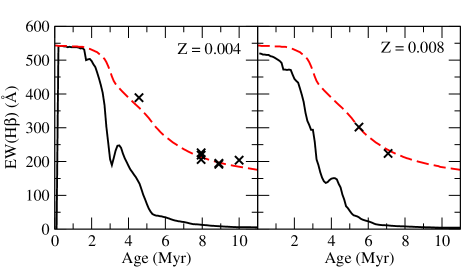
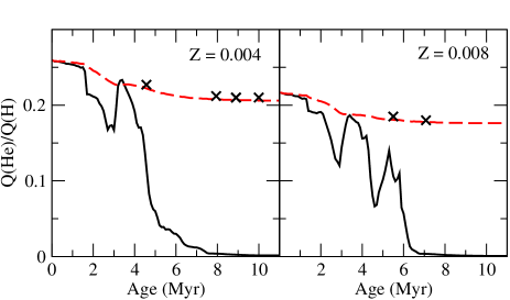
Figure 5: Left panels: relation between the equivalent width of H$\beta$ and the age of the corresponding synthesis population model for metallicities of 0.004 and 0.008 as predicted by Starburst99. Crosses represent the observed values measured on the young stellar continua and multiplied by the corresponding absorption factor obtained in each tailor-made model. The assigned age to each object is that predicted by the same models. Therefore, the J1540 point does not appear as the fitted age is older than 10 Myr. Right panels: relation between the ratio of helium to hydrogen ionizing photons and the age of the ionizing cluster. In all panels, the black solid line represents an instantaneous star formation and the red dashed line, a continuous star formation as predicted by Starburst99. As in the previous case, crosses represent the values obtained from the models for each object, with the exception of J1540.

Regarding the age of the burst, the equivalent width of an intense Balmer emission line, like H$\beta$, is generally associated to the age and properties of the ionizing population. It has long been accepted that the low values of EW(H$\beta$) found in starburst galaxies as compared with the predictions from Population Synthesis Models are due to the presence of an underlying stellar population that enhances the continuum light without significantly contributing to the ionization of the gas. Nevertheless, as can be seen in Table 2 the subtraction of this population from the integrated spectra does not imply significant corrections to EW(H$\beta$) (between 1.5 % in the case of J1540 and J1729 and 24 % in the case of J0032).

However, the excitation conditions found in these objects, are only reachable with the energy supplied by very young and massive O stars, whose associated EW(H$\beta$) is four or five times larger than the observed values. This difference can be partially explained by a certain dust absorption of UV photons. The dust absorption factors obtained in our models range between 1.5 and 2, as we can see in Table 6. These help to put the modeled EW(H$\beta$) values in agreement with the observed ones.

In the left panels of Figure 5 we show the evolution of EW(H$\beta$) with time for the two metallicities closest to those in our sample for both instantaneous (black solid line) and continuous (dashed red line) star formation laws as obtained from Starburst99 models. In the right panels of the same figure we show the evolution of the ratio of helium to hydrogen ionizing photons, Q(He)/Q(H) according to the same Starburst99 models. This ratio, that can be considered a good estimate of the ionizing power of the cluster, falls dramatically for an instantaneous star formation law once the WR phase has finished ($\sim$ 5 Myr), while it maintains a constant high value in the case of a continuous star formation. We can compare these diagrams with the observed EW(H$\beta$), once the underlying stellar population has been removed and the dust absorption factor has been taken into account. They appear as crosses in Figure 5 and lie in a range which corresponds to the asymptotic value of the continuous star formation line. In the case of the evolution of Q(He)/Q(H), crosses represent the values derived from the tailor-made models.

Although it is true that both EW(H$\beta$) and Q(He)/Q(H) could be consistent with an instantaneous burst at present in the WR phase, statistically it is not probable that all the objects of the sample present such similar properties due to their being in the same evolutionary stage. At the same time, all the calculated photoionization models in our work require a great amount of O and B stars younger than the WR phase in order to reach the ionization conditions responsible for the observed emission lines. We have therefore assumed for all the studied objects a continuous star formation history for the ionizing source, with a duration longer in all cases than 5 Myr.

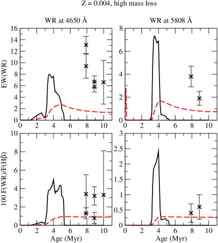
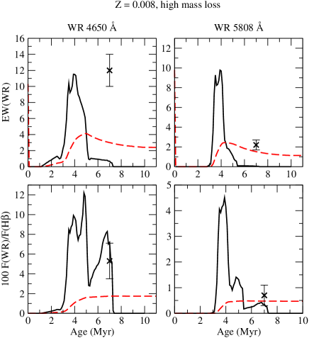
Figure 6: Relation between the WR equivalent widths and relative intensities of both the blue and the red bumps as a function of the age of the cluster, according to Starburst99 model predictions, at left for a metallicity of Z = 0.004 and at right for Z = 0.008. In all panels, black solid lines represent the instantaneous star formation model and red dashed lines the continuous star formation one. Crosses represent the corrected values derived for each galaxy and listed in Table 3

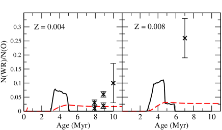
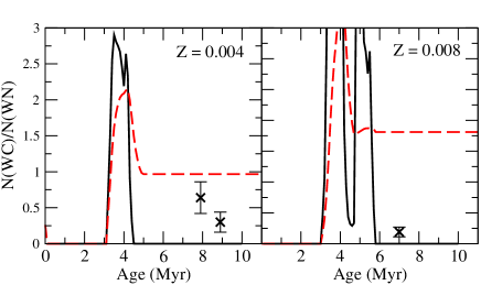
Figure 7: Left panels: time evolution of the ratio of WR to O stars according to Starburst99 predictions. Right panel: same but for the ratio of WC to WN stars. In both cases, results for two metallicities, Z= 0.004 and Z=0.008, are shown. Solid lines represent instantaneous star formation models and dashed line continuous star formation ones. Crosses represent the derived numbers for each galaxy taking into account the measured luminosities of the bumps as compared with those predicted by the Starburst99 models at the predicted age. The number of O stars has been derived using the same procedure for L(H$\alpha$).

4.2 Derived properties of the WR population

Seven out of the ten observed galaxies have detectable WR features in their spectra. Five of them were already included in the catalog by Kniazev et al. (2004; SHOC) with a flag indicating the detection of both the blue and red bumps from WR stars. In our spectra, the red bump is observed in only three galaxies. The SHOC catalog, however, does not provide actual measurements for the features. In a more recent paper, Brinchmann et al. (2008) list only the ”blue bump” luminosities and equivalent widths of three galaxies from the present work: J002101 (SHOC 11), J003218 (SHOC 22) and J162410 (SHOC 536). The direct comparison between the equivalent widths of the blue bump measured by these authors inside the 3-arcsec fiber spectra of the SDSS and our long-slit observations yields discrepancy factors for J0021, J0032 and J1624 of 1.7, 2.0 and 1.1, respectively, larger in our WHT observations. This could be a consequence of the smaller aperture of our long-slit observations which includes a lower contribution to the continua from extended ionized gas and hence produce larger equivalent widths.

Table 7 shows the extinction corrected luminosities of the measured WR bumps. We show in the same table the number of O and WR stars as derived from the extinction corrected H$\alpha$ and WR blue bump luminosities, respectively. In the case of O stars, we have taken into account as well the dust absorption factor, $f_{d}$. The total number of stars have been estimated by comparison with the properties of the Starburst99 models at the age derived from the photoionization models described above. For those galaxies with a red bump detection we have used the same libraries to derive the ratio between WC and WN stars, which is also listed in Table 7.

Table 7: Luminosities of the Wolf-Rayet features measured for the sample of HII galaxies at 4650 Å (blue bump, bb) and at 5808 Å (red bump, rb), derived number of WR stars, ratios of WR to O stars and, for those galaxies with a detection of the red bump, of WC to WN stars.

Object ID	log L(bb)	log L(rb)	N(WR)	WR/O	WC/WN
	(erg $\cdot$ s-1)	(erg $\cdot$ s-1)
J0021	39.84$\pm$0.09	–	2500$\pm$600	0.02$\pm$0.01	–
J0032	38.53$\pm$0.08	37.79$\pm$0.16	150$\pm$30	0.06$\pm$0.01	0.30$\pm$0.14
J1509	39.73$\pm$0.09	38.84$\pm$0.11	1750$\pm$400	0.11$\pm$0.02	0.19$\pm$0.08
J1540	38.18$\pm$0.06	–	60$\pm$15	0.26$\pm$0.07	–
J1616	37.32$\pm$0.23	–	9$\pm$6	0.10$\pm$0.07	–
J1624	39.46$\pm$0.08	38.92$\pm$0.12	1070$\pm$200	0.03$\pm$0.01	0.64$\pm$0.22
J1729	38.92$\pm$0.12	–	300$\pm$100	0.01$\pm$0.01	–

We can compare the relative intensities and equivalent widths of the WR bumps detected in our objects with the predictions of Starburst99 populations synthesis models as a function of the metallicity, age and star formation law of the cluster. To make this comparison we have taken the corrected values listed in Table 3: in the case of EWs from the effect of the underlying stellar populations and the contribution of the nebular continuum and in the case of the relative intensities from the effect of the dust absorption factor to the hydrogen recombination lines. In Figure 6 we show the predicted equivalent widths and intensities relative to H$\beta$ of both the blue and red bumps as a function of the age of the cluster for metallicities Z = 0.004 (0.2$\cdot$Z_⊙), left panels, and Z = 0.008 (0.4$\cdot$Z_⊙), right panels. The black solid lines represent the evolution of an instantaneous burst, while the red dashed lines do for a continuous star formation history with a constant star formation rate. Crosses represent the corrected values as listed in Table 3 with their corresponding error bars. As we can see, the models predict the brightest and most prominent features for the highest metallicity, agreeing with the stellar model atmospheres for WR stars (Crowther, 2007 and references therein). At the same time, we can appreciate that in the instantaneous star formation case the WR features appear during a time interval between 2 and 5 Myr reaching higher intensities than in the case of continuous star formation. In this latter scenario, the WR features appear at the same age and, despite reaching lower intensities, they converge to a non-zero value at older ages. For an average metallicity between the two cases of study these values are EW $\sim$ 2 Å and 0.013$\cdot$I(H$\beta$) for the blue bump and EW $\sim$ 1 Å and 0.004$\cdot$I(H$\beta$) for the red one. By comparing with the measured relative intensities and equivalent widths in our sample objects we can see that all of them are larger than the Starburst99 model predictions for a constant star formation law and, in some of them, like J1509 and J1540, even larger than the values predicted for an instantaneous burst.

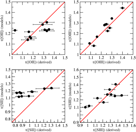
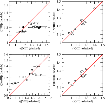
Figure 8: Comparison between the electron temperatures (in units of 10⁴ K) as derived from the observations and from the tailor-made photoionization models. Black circles represent a comparison between a temperature directly derived in the observations, while white squares represent a temperature of another ion, assumed to be similar in the thermal structure.

A great deal of work has been done in order to reconcile this disagreement between the observed luminosities of the WR bumps detected in the integrated spectra of galaxies and the model stellar atmospheres of WR stars and evolutionary synthesis models of clusters. Suggested hypotheses include the existence of a binary channel (Eldridge et al., 2007) or the consideration of rotation in the stellar evolutionary tracks, which reduces the mass required to form WR stars (Meynet & Maeder, 2005). Nevertheless, some other reasons can be explored such as geometrical effects. If we consider the whole burst of star formation and we assume a continuous star formation law, we must compare the luminosities of the WR bumps with the intensities of the Balmer lines and the continuum coming from the whole burst. This approach was already used by Pérez-Montero & Díaz (2007) to match the observed fluxes of the WR features in Mrk 209. On the contrary, if only the ionizing stellar population producing the WR stars is considered, only the burst region where the WR population concentrates must be analyzed. This could explain as well the lack of WR emission in the other three galaxies with an assumed continuous star formation history. In the case of our sample, no aperture correction factors have been taken into account either for the H$\alpha$ luminosities or the continuum contribution at the WR bumps wavelength, due to the compact nature of the objects. Indeed, the discrepancy factors between our H$\alpha$ luminosities and those measured in the SDSS catalogue using a 3 arcsec fiber is not larger than 1.5 in any case and even smaller than 1 in two of them (J1528 and J1729). Therefore, the aperture factor does not seem to be the cause of the abnormally high values found for the EW and the relative intensities of the WR features.

The analysis of the relative number of WR to O stars and of the number of WC to WN stars leads to very similar conclusions. In all cases the derived ratio of the number of WR to O stars is much higher than the asymptotic value reached with a continuous star formation, which is 0.022 for a metallicity in between the two studied cases. For J1540, the obtained value, 0.44, is even much higher than the value expected for an instantaneous burst. As in the case of the luminosities of the WR features, we can reconcile the derived values enhancing the number of O stars on the basis that a non-negligible flux of the radiation from these stars is obscured by internal extinction. As in the previous case, probably geometrical effects can be determinant. Regarding the ratio between WC and WN stars, the derived values are lower in all cases than expected. This is due to the fact that the luminosities of the red bump predicted by the models are in much better agreement with the observed values than those of the blue bump and, hence, the relative number of WC stars is lower.

4.3 Physical conditions and ionic abundances of the gas through tailor-made models

The correct determination of ionic abundances in ionized gaseous nebulae using collisional emission lines versus recombination lines has become a matter of debate in the last years due to the disagreements predicted by photoionization models in the high metallicity regime (e.g. Charlot & Longhetti, 2001) or the discrepancies found in local nebulae (e.g. Peimbert et al., 2007 and references therein).

Many times, these discrepancies are due to the simple assumptions made about the ionization structure of the nebulae. Indeed, the only electron temperature measured in many cases is t([Oiii]) because the emission line of [Oiii] at 4363 Å is the brightest auroral line. This temperature is assumed to be representative of the high excitation zone and the low excitation zone temperature is obtained under very simple assumptions. This can produce large deviations in high metallicity nebulae, where the low excitation ions have a high relative weight in the total abundance of a specific species (Pérez-Montero & Díaz, 2005). One way to overcome this issue is to try to trace as precisely as possible the inner thermal structure of the gas.

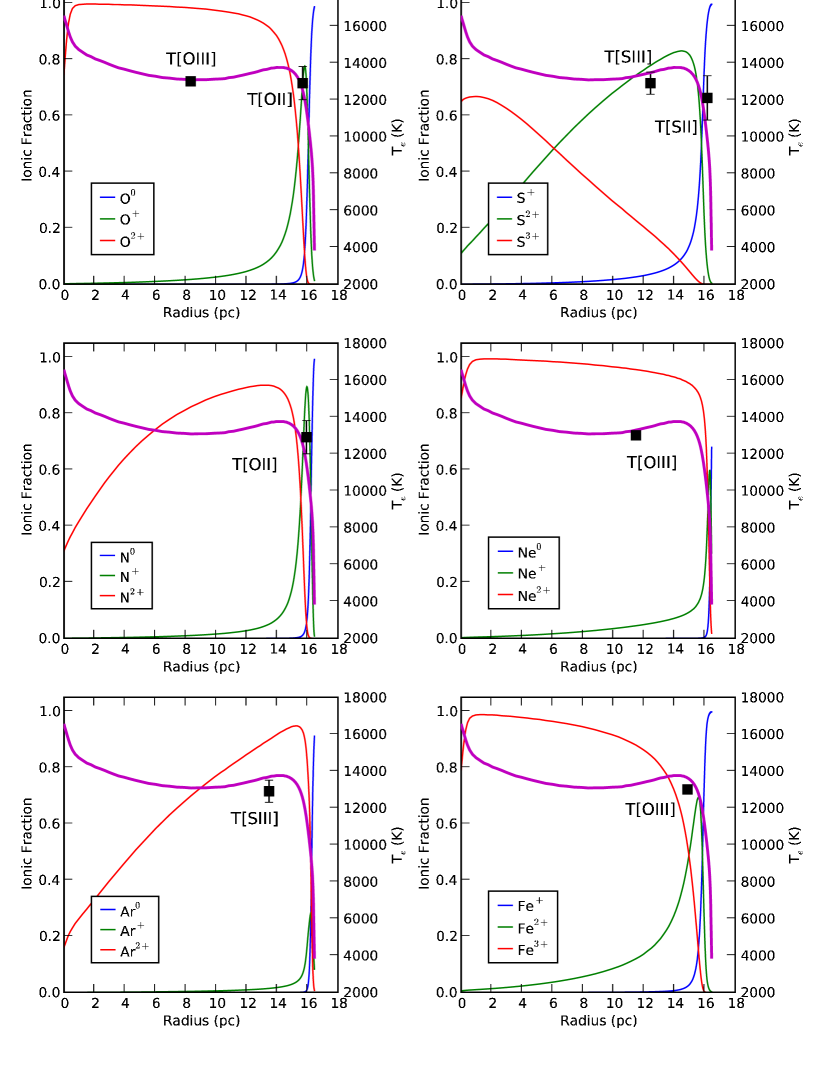
Figure 9: Radial profile of the electron temperature, in violet solid line, and the relative abundance of different ionic species (from left to right and up to down, O, S, N, Ne, Ar and Fe) as calculated in the best photoionization tailor-made model of the galaxy J1616. We show as well the derived electron temperatures of oxygen and sulphur as black squares in the position of the average abundance of the corresponding ions.

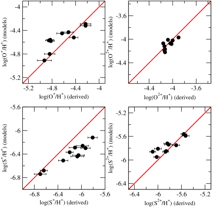
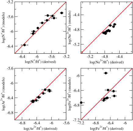
Figure 10: Comparison between ionic abundances as derived from the observations using the direct method and the predictions of tailor-made photoionization models.

In Figure 8 we show a comparison between derived and modeled temperatures for the objects of our sample, for which at least four electron temperatures have been measured. In the case of ions whose temperatures can not be derived due to the lack of observable lines in the optical, another line temperature, assumed to be representative of the zone where these iones are formed, has been used: t([Siii]) in the case of [Ariii], t([Oiii]) in the case of [Neiii] and [Feiii] and t([Oii]) in the case of [Nii] in the objects where this was not available. As we can see, the agreement for t([Oiii]) is excellent, mostly due to the input conditions in the models to fit the auroral line of [Oiii]. Regarding t([Oii]) and t([Siii]), the agreement is still good, although slightly worse that in the previous case. Finally, the largest deviations are found for the electron temperature of [Sii]. Except in the cases of J1455 and J1616, models predict much higher temperatures than observed. This is not surprising if we take into account that the emission of [Sii] is often found as well in the diffuse medium (e.g. Hunter & Gallagher, 1990) and therefore we are probably tracing in our observations a non-negligible portion of colder and less dense gas, which has not been considered in our models. This is compatible with the significatively lower radii found in our models in comparison with the values obtained from the spatial profile of H$\alpha$. Perhaps, this could be overcome if we considered in our models a low-density region in the outer parts of the nebula where lines from low excitation ions like [Sii] were produced. In the case of the three objects with a measurement of the electron temperature of [Nii], the agreement is rather good in the case of J0021, while it is sensibly underestimated by the models in the case of J1624 and J1729. This temperature is assumed to be equal to t([Oii]) in objects without a measurement of the auroral line of [Nii] at 5755 Å. As we can see in the corresponding panel, this assumption seems to work for most of the objects, except in the cases of J0032 and J1455. For these objects, we can not rule out some geometrical effect not considered in our photoionization models.

For the rest of assumptions, as t([Ariii]) $\sim$ t([Siii]) or t([Neiii]) $\sim$ t([Feiii]) $\sim$ t([Oiii]), we can see that all of them work fairly well.

In Figure 9 we illustrate the good agreement found between models and observations for the galaxy J1616. In each panel, in red, green and blue solid lines, the radial distribution of the ionic fractions of the different elements as computed by the model (from left to right and from up to down: O, S, N, Ne, Ar and Fe) are plotted. The magenta thick solid lines show the radial distribution of the electron temperature predicted by the same model. Finally, black squares show the electron temperatures obtained from the observations. We have associated these points to the average zone where the corresponding ion is formed. In the cases of Ne²⁺ and Fe²⁺, t([Oiii]) is shown; for Ar²⁺, t([Siii]) is plotted and in the cases in which no measurements of t([Nii]) are available, this is represented by t([Oii]).

In Figure 10, we show the comparison between the relative ionic abundances, derived using the corresponding measured electron temperatures and the observed emission-line intensities, and the same abundances as predicted by our photoionization models. We can see that the agreement is somewhat better for high excitation ions, like O²⁺, than for low excitation ones, like O⁺ and S⁺. At the same time these latter ions present abundances spanning a wider range than the former. This might indicate that geometrical effects (e.g. density variations, matter bounded nebulae, etc…) affect the diagnostics of the gas in the low excitation region, hence a simple scheme can not be adopted for its analysis. In the case of our sample of HII galaxies, these differences are not appreciable due to their low metallicities and high excitation conditions, so the inner parts have a large weight on their average conditions. On the contrary, the analysis of disk HII regions and high metallicity objects are tied to a much larger uncertainty if these effects are not taken into account using as many indicators of the physical conditions of the gas as possible.

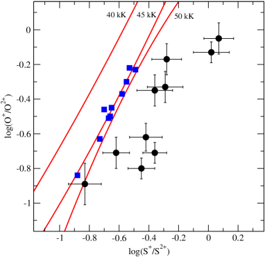
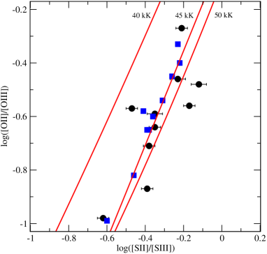
Figure 11: At left, relation between the ratio of ionic abundances S⁺/S²⁺ and O⁺/O²⁺, whose quotient is the $\eta$ parameter. Black dots with error bars represent the modeled objects with the corresponding derived ratios, while blue squares are the values derived from the models. Red solid lines represent the fits to a sequence of photoionization models with the same effective temperature. The right panel represents the relation between the ratios of [SII]/[SIII] and [OII]/[OIII]. Symbols are the same as in left panel.

4.4 The hardening of the radiation

The stellar effective temperature has been traditionally the functional parameter most difficult to obtain. Vílchez & Pagel (1988) defined the so-called softness parameter, $\eta$, which allows to estimate the hardening of the radiation field by means of the ratio of the ionic abundances of oxygen and sulphur, derived from the optical spectrum.

$$\eta=\frac{O^{+}/O^{2+}}{S^{+}/S^{2+}}$$ (5)

The same ratio, defined using the intensities of the corresponding emission lines, can also be used to figure out the scale of equivalent effective temperature:

$$\eta^{\prime}=\frac{[OII]3727/[OIII]4959,5007}{[SII]6717,6731/[SIII]9069,9532}$$ (6)

Both expressions agree in finding that HII galaxies present very high equivalent effective temperatures as compared to other HII regions of higher metallicity. Nevertheless, there is a disagreement between the position of these objects in diagnostic diagrams and the scale of temperatures of the stellar atmospheres of O stars. HII galaxies usually lie in a region of the diagrams which corresponds to temperatures even higher than the maximum value of model atmospheres, which is 50 kK. The cause has been sometimes attributed to some extra source of heating in HII galaxies (e.g. Stasińska & Schaerer, 1999).

The left panel of Figure 11 shows the logarithmic ionic fractions O⁺/O²⁺ vs. S⁺/S²⁺. The different lines of constant slope 1 in this diagram correspond to different values of the $\eta$ parameter and hence of ionizing radiation temperature. The values derived from actual measurements of our observed objects are plotted as black solid circles while blue squares correspond to the values derived from the computed models. Red solid lines represent polynomial fits to different photoionization models computed using as ionizing source WM-Basic stellar atmospheres (Pauldrach et al., 2001) for different values of the effective temperature. These model sequences can help to establish the scale of the equivalent effective temperature. We can see that the models are not able to reproduce the high values of log(S⁺/S²⁺), and in some cases log(O⁺/O²⁺) found in our objects that, in fact, would correspond to extremely high values of equivalent effective temperatures.

This disagreement disappears when the emission lines instead of the actual ionic ratios are considered. This is due to the fact that emission-line intensities are well fitted in all the tailor-made models while this is not the case for electron temperatures (see Figure 8), specially for T([SII]) which is, in general overestimated by the models leading to an underestimate of the S⁺/H⁺ abundance ratio. Again, the disagreement could be caused by the geometry of the diffuse gas in these HII regions, which is not adequately modeled, thus avoiding the need for an extra source of heating to explain the apparently high stellar effective temperatures in these objects. At the same time, this probably means that the calibration of the effective temperature is not unique but in fact sensitive to the object class involved, through the different geometries of the ionized gas.

5 Summary and conclusions

We have studied the underlying and ionizing stellar populations and have modeled the properties of the emitting gas in a sample of HII galaxies. This sample was observed (H06 and H08) using double-arm spectrographs, which allow the simultaneous analysis of the entire spectral range from [OII] 3727 Å to [SIII] 9532 Å providing the derivation of the electronic temperatures of, at least, four ions in all the cases: O⁺, O²⁺, S⁺, and S²⁺ and hence a precise determination of the ionization structure of the gas.

The fitting of the blue part of the continuum was made using the program STARLIGHT and the SEDs computed from the Starburst99 stellar population synthesis models. This approach was used to study in a consistent manner the differences between the stellar populations in our sample of galaxies. The resulting distribution of ages and masses from this fitting revealed the presence of various stellar populations. An underlying stellar population of about several Gyr dominates the stellar mass, while the blue to visual light is in all cases dominated by young stellar populations with ages younger than 10 Myr. The presence of the older population can affect the reddening determination but its contribution to the measured EW(H$\beta$) is only about 10% for most of the sample objects, being around 25% in the case of J0032 and almost zero for J1616 and J1729. In fact, regarding the subtraction of Balmer absorption features from the underlying stellar populations, we did not find that the spectral fitting technique constitute a substantial improvement over the simultaneous fitting of absorption and emission components as performed in previous works (H06 and H08).

We analysed the Wolf-Rayet clusters detected in seven of the ten studied galaxies through the WR broad features seen in their spectra. The fitting of the stellar population and the modeling of the ionized gas allows to correct them for the contribution of the underlying population and the nebular emission to the continuum and for the dust absorption factor in the case of the emission of the Balmer lines. The comparison between the corrected fluxes and equivalent widths of the WR blue bump with the predictions from Starburst99 models at the corresponding metallicity leads to the estimate of the number of WR stars which ranges from 9$\pm$6 to 2500$\pm$600 depending on the galaxy. In three of them, also the red bump was measured allowing to estimate the WC to WN number ratio, Nevertheless, the fluxes of both the blue and red bumps relative to H$\beta$ are larger than the values predicted by the models in almost all the cases.

A continuous star formation history of the stellar ionizing population has been assumed in all the objects of the sample. This is supported by the simultaneous presence of very massive O and WR stars, along with the relatively low measured values of EW(H$\beta$), once corrected for underlying contribution and dust absorption. The ages of the star formation bursts, the number of ionizing photons as derived from the H$\alpha$ fluxes and the intensities of the most prominent emission lines were used to constrain photoionization models for each galaxy. The Starburst99 libraries were used to calculate the SED of the ionizing cluster in order to be consistent with the previous fitting of the stellar populations. Some dust is assumed to be present associated with the gas. The amount of dust in each model was derived in order to reproduce the observed EW(H$\beta$). These derived values agree well with the main observed quantities in each object, with the exception of the sizes of the ionized regions which result 5-10 times smaller in the models as compared to measurements from H$\alpha$ in the spatial profiles of the slits.

The observed electron temperatures and ionic abundances are, in most cases, well reproduced by the models which implies that the direct method using collisional emission lines provides robust answers if the thermal structure of the nebula is well traced. Therefore, our models were able to reproduce the ionization structure of the nebula without appealing to temperature fluctuations or any other geometrical effects that can affect the abundances derived from collisionally excited emission lines. This result is consistent with the temperature measured from the Balmer jump in some of the objects in our sample (H06). Only the electron temperature and the ionic abundances of S⁺/H⁺ is not well reproduced by our models, which could be consequence of the presence of diffuse gas in these galaxies, not taken into account in the models. This would also be consistent with the small sizes predicted by the models as compared with H$\alpha$ spatial profiles in the slits.

Finally, regarding the hardness of the radiation field, model predictions agree with observations when the softness parameter $\eta$, which parametrizes the temperature of the ionizing radiation, is expressed in terms of emission line intensity ratios. However, there is a disagreement when ionic abundance ratios are used instead. This is probably caused by the overestimate of the electron temperature of S⁺ by the models and the corresponding underestimate of the S⁺/S²⁺ abundance ratio rather than by existence of an additional heating source in HII galaxies.

Appendix A Total abundances and ionization correction factors

The calculation of tailor-made photoionization models for each galaxy with a reliable inner ionization structure based on the measurement of various electron temperatures allows a complete description of the total abundances of the main elements present in the gas. With this information it is possible to compare the ionization fractions obtained from the models with the most widely used ionization correction factors (ICFs), necessary to derive the total abundances of certain elements for which there are no lines in the optical range for all the main ionization stages. Generally, for an ionic species $X^{+i}$, whose abundance has been derived from forbidden collisional lines, we define the ICF for that ion in the following manner:

$$\frac{X}{H}=ICF(X^{+i})\cdot\frac{X^{+i}}{H^{+}}$$ (7)

In Table LABEL:icfs we list the total abundances and the ICFs obtained from the models for N, S, Ne, Ar and Fe.

Table 8: Ionization correction factors and total abundances as derived from photoionization models of the main elements with emission lines in the optical spectral range of the studied HII galaxies.

	J0021	J0032	J1455	J1509	J1528	J1540	J1616	J1624	J1657	J1729
12+log(O/H)	7.99	8.01	7.94	8.18	8.18	8.15	8.00	8.04	8.01	8.12
ICF(N+)	4.17	4.79	6.61	5.13	3.80	3.47	9.78	5.13	3.39	5.37
12+log(N/H)	7.13	6.78	6.76	7.01	7.00	6.90	6.62	6.71	6.76	7.16
ICF(S++S2+)	1.11	1.14	1.28	1.12	1.10	1.04	1.37	1.16	1.07	1.19
12+log(S/H)	6.29	6.40	6.23	6.57	6.41	6.54	6.33	6.30	6.34	6.41
ICF(Ne2+)	1.20	1.17	1.10	1.20	1.23	1.29	1.07	1.15	1.26	1.15
12+log(Ne/H)	7.24	7.24	7.16	7.36	7.43	7.22	7.17	7.22	7.19	7.37
ICF(Ar2+)	1.15	1.17	1.23	1.15	1.15	1.10	1.29	1.17	1.15	1.17
ICF(Ar2++Ar3+)	1.05	1.06	1.03	1.04	1.07	1.06	1.02	1.04	1.08	1.04
12+log(Ar/H)	5.58	5.69	5.58	5.87	5.78	5.82	5.64	5.68	5.57	5.79
ICF(Fe2+)	2.69	2.88	3.89	2.95	2.57	2.14	5.13	3.09	2.40	3.24
12+log(Fe/H)	5.82	5.80	5.86	5.92	5.99	5.73	6.15	5.77	5.79	5.88

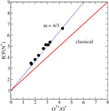
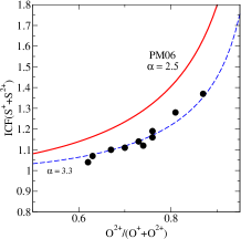
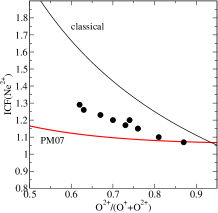
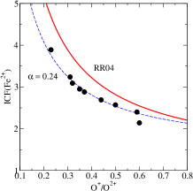
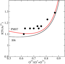
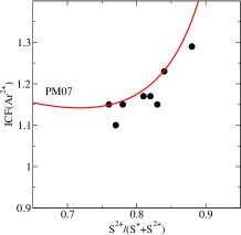
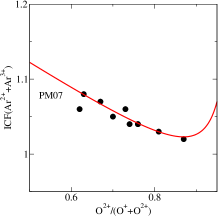
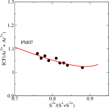
Figure 12: Comparison between different ionization correction factors (ICFs) derived for different elements from the computed photoionization models (black circles) and some of the most used relations.

The oxygen ionic abundance ratios, O⁺/H⁺ and O²⁺/H⁺, usually derived from the [Oii] $\lambda\lambda$ 3727,29 Å and [Oiii] $\lambda\lambda$ 4959, 5007 Å lines are related to the total abundance of oxygen assuming that:

$$\frac{O}{H}\,\approx\,\frac{O^{+}+O^{2+}}{H^{+}}$$ (8)

which is based on the assumption that the relative abundances of neutral hydrogen and oxygen are similar. We have checked in our models that this assumption is valid within a 1% of uncertainty. As the bright emission lines of oxygen are well reproduced by our models, as also is the temperature sensitive line, the agreement between the total oxygen abundances derived from observations and models agree fairly well with deviations, in most cases, no larger than the reported observational errors.

The total abundance of nitrogen is obtained from the ionic abundance of N⁺, derived from the intensities of the $\lambda\lambda$ 6548, 6584 Å lines. Then, a similar ionization structure for nitrogen and oxygen is assumed, according to the following expression:

$$\frac{N}{O}\,\approx\,\frac{N^{+}}{O^{+}}$$ (9)

which, combined with equation (6), leads to the following ICF for nitrogen:

$$ICF(N^{+})=1+\frac{O^{2+}}{O^{+}}$$ (10)

In the top left panel of Figure 12 we plot these ICFs as a function of the O⁺/O²⁺ ratio as compared to the best linear fit to the models. The slope of the fit is slightly higher (1.33), than the value derived using the classical assumption. This is a consequence of the fact that the ionic fraction of N⁺ is lower than that of O⁺ in these type of objects.

Regarding sulphur, we have derived S⁺/H⁺ abundances from the fluxes of the [Sii] emission lines at $\lambda\lambda$ 6717, 6731 Å and T([Sii]) and S²⁺/H⁺ abundances from the fluxes of the near-IR [Siii] $\lambda\lambda$ 9069,9532 Å lines and T([Siii]). The total sulphur abundance has been calculated using an ICF for S⁺+S²⁺ according to Barker’s (1980) formula, which is based on the photoionization models of Stasińska (1978). We have written this formula as a function of the ratio O²⁺/O instead of O⁺/O in order to reduce the propagated error for this quantity.

$$ICF(S^{+}+S^{2+})\approx\left[1-\left(\frac{O^{2+}}{O^{+}+O^{2+}}\right)^{\alpha}\right]^{-1/\alpha}$$ (11)

where $\alpha$ = 2.5 provides the best fit to the scarce observational data on S³⁺ abundances (Pérez-Montero et al. 2006, PM06 in the plot). Nevertheless, we can see in Figure LABEL:icfs that a value of $\alpha$ = 3.3 provides a better fit to the results obtained from the photoionization models.

Neon is only visible in the spectra by means of the [Neiii] emission line at $\lambda$3869 Å. The total abundance of neon has been calculated using the following expression for the ICF (Pérez-Montero et al., 2007, PM07 in the plots):

$$ICF(Ne^{2+})\approx 0.753+0.142\cdot\frac{O^{2+}}{O^{+}+O^{2+}}+0.171\cdot\frac{O^{+}+O^{2+}}{O^{2+}}$$ (12)

This formula takes into account the overestimate of Ne/H in objects with low excitation, where the charge transfer between O²⁺ and H⁰ becomes important (Izotov et al., 2004, I04 in the plot). Nevertheless, the total abundances obtained in our models are slightly higher than those derived with the use of this ICF.

The only available emission lines of argon in the optical spectra of ionized regions are those of [Ariii] at 7136 Å and [Ariv] at 4740 Å. It is usually assumed that T([Ariii]) $\approx$ T([Siii]) (Garnett, 1992). The total abundance of Ar can be calculated using the ICF(Ar²⁺) derived from photo-ionization models by Pérez-Montero et al. (2007, PM07 in the plots), in the case that only the emission line of [Ariii] be detected

$$ICF(Ar^{2+})\,=0.749+0.507\cdot\Big{(}1-\frac{O^{2+}}{O^{+}+O^{2+}}\Big{)}+$$

$$+0.0604\cdot\Big{(}1-\frac{O^{2+}}{O^{+}+O^{2+}}\Big{)}^{-1}$$ (13)

In the same work, another ICF is proposed for the case in which [Ariv] is also measured:

$$ICF(Ar^{2+}+Ar^{3+})=0.928+0.364\cdot(\Big{(}1-\frac{O^{2+}}{O^{+}+O^{2+}}\Big{)}+$$

$$+0.006\cdot\Big{(}1-\frac{O^{2+}}{O^{+}+O^{2+}}\Big{)}^{-1}$$ (14)

These two ICFs can be expressed as well as a function of the ionic abundances of sulphur, S⁺ and S²⁺, when only red spectroscopic observations are available:

$$ICF(Ar^{2+})\,=0.596+0.967\cdot\Big{(}1-\frac{S^{2+}}{S^{+}+S^{2+}}\Big{)}+$$

$$+0.077\cdot\Big{(}1-\frac{S^{2+}}{S^{+}+S^{2+}}\Big{)}^{-1}$$ (15)

$$ICF(Ar^{2+}+Ar^{3+})=0.870+0.695\cdot(\Big{(}1-\frac{S^{2+}}{S^{+}+S^{2+}}\Big{)}+$$

$$+0.0086\cdot\Big{(}1-\frac{S^{2+}}{S^{+}+S^{2+}}\Big{)}^{-1}$$ (16)

In the bottom panels of Figure 12, we can see that the agreement between these expressions and the ICFs found in our models is good.

Finally, iron abundances in the gas-phase can be calculated by correcting the ionic abundances of Fe²⁺, derived from the intensity of the emission line of [Feiii] at 4658 Å, using the following expression from Rodríguez & Rubin (2004, RR04 in the plot):

$$ICF(Fe^{2+})=\left(\frac{O^{+}}{O^{2+}}\right)^{\alpha}\cdot\left[1+\frac{O^{2+}}{O^{+}}\right]$$ (17)

with a value of $\alpha$ = 0.09. Nevertheless, the fit to the ICFs found in our models gives a best value for $\alpha$ = 0.24, which leads to lower total abundances of iron.

References

- [Asplund et al.(2005)] Asplund, M., Grevesse, N., & Sauval, A. J. 2005, Cosmic Abundances as Records of Stellar Evolution and Nucleosynthesis, 336, 25
- [1] Badnell, N. R., 2006, A&A, 447, 389
- [2] Baldwin, J.A. Phillips, M.M., Terlevich, R., 1981, PASP, 93, 5
- [3] Barker, T., ApJ, 1980, 240, 99
- [4] Bell, E.F. & de Jong, R.S., 2001, ApJ, 550, 212
- [Brinchmann et al.(2008)] Brinchmann, J., Kunth, D., & Durret, F. 2008, A&A, 485, 657
- [5] Charlot, S. & Longhetti, M. 2001, MNRAS, 323, 887
- [Cid Fernandes et al.(2004)] Cid Fernandes, R., Gu, Q., Melnick, J., Terlevich, E., Terlevich, R., Kunth, D., Rodrigues Lacerda, R., & Joguet, B. 2004, MNRAS, 355, 273
- [6] Conti P.S., 1991, ApJ 377, 115
- [7] Crowther, P. A., 2007, ARA&A, 45, 177
- [8] Díaz, A.I. 1988, MNRAS, 231, 57
- [9] Díaz, A.I. 1998, Ap&SS, 263, 143
- [10] Díaz, A. I., Terlevich, E., Vílchez, J. M., Pagel, B. E. J., & Edmunds, M. G.: 1991, MNRAS, 253, 245
- [Eldridge et al.(2008)] Eldridge, J. J., Izzard, R. G., & Tout, C. A. 2008, MNRAS, 384, 1109
- [11] Ferland, G. J., Korista, K.T., Verner, D.A., Ferguson, J.W. Kingdon, J.B. & Verner, E.M. 1998, PASP, 110, 761
- [12] French, H.B. 1980, ApJ, 240, 41
- [Guseva et al.(2006)] Guseva, N. G., Izotov, Y. I., & Thuan, T. X. 2006, ApJ, 644, 890
- [Hägele et al.(2008)] Hägele, G. F., Díaz, A. I., Terlevich, E., Terlevich, R., Pérez-Montero, E., & Cardaci, M. V. 2008, MNRAS, 383, 209 (H08)
- [Hägele et al.(2006)] Hägele, G. F., Pérez-Montero, E., Díaz, A. I., Terlevich, E., & Terlevich, R. 2006, MNRAS, 372, 293 (H06)
- [13] Garnett, D.R. 1992, AJ, 103, 1330
- [14] Guseva, N.G., Izotov, Y.I., Thuan, T.X. 2006, ApJ, 644, 890
- [Hunter & Gallagher(1990)] Hunter, D. A., & Gallagher, J. S., III 1990, ApJ, 362, 480
- [15] Izotov, Y. I., Stasińska, G., Meynet, G., Guseva, N. & Thuan, T.X., 2006, A&A, 448, 955
- [16] Kewley, L. J. & Ellison, S. L. 2008, ApJ, 681, 1183
- [17] Kniazev, A.Y., Grebel, E.K., Hao, L. et al. 2003, ApJL, 593, L73
- [18] Kroupa, P.: 2002, Science 295, 82
- [19] Lamareille, F., Mouhcine, M., Contini, T., Lewis, I. & Maddox, S., 2004, MNRAS, 350, 396
- [20] Larson, R.B. 1974, MNRAS, 169, 229
- [Lebouteiller et al.(2008)] Lebouteiller, V., Bernard-Salas, J., Brandl, B., Whelan, D. G., Wu, Y., Charmandaris, V., Devost, D., & Houck, J. R. 2008, ApJ, 680, 398
- [Leitherer et al.(1992)] Leitherer, C., Robert, C., & Drissen, L. 1992, ApJ, 401, 596
- [21] Leitherer, C., Schaerer, D., Goldader, J. D., Delgado, R. M. G., Robert, C., Kune, D. F., de Mello, D. F., Devost, D., and Heckman, T. M.: 1999, ApJSS. 123, 3
- [Lequeux et al.(1979)] Lequeux, J., Peimbert, M., Rayo, J. F., Serrano, A., & Torres-Peimbert, S. 1979, A&A, 80, 155
- [22] López, J. 2005, MSc Thesis, INAOE
- [Mateus et al.(2006)] Mateus, A., Sodré, L., Cid Fernandes, R., Stasińska, G., Schoenell, W., & Gomes, J. M. 2006, MNRAS, 370, 721
- [23] Mathis, J.S., Rumpl, W. & Nordsieck, K.H. 1977, ApJ, 217, 425 (MRN)
- [24] Meynet, G. & Maeder, A., 2005, A&A, 429, 485
- [25] Meynet, G., Maeder, A., Schaller, G., Schaerer, D., & Charbonnel, C.: 1994, A&ASS 103, 97
- [26] Osterbrock, D. E. 1989, Astrophysics of gaseous nebulae and active galactic nuclei, Mill Valley, CA, University Science Books
- [Olive & Skillman(2004)] Olive, K. A., & Skillman, E. D. 2004, ApJ, 617, 29
- [27] Pauldrach, A.W.A., Hoffmann, T.L. & Lennon, M. 2001, A&A, 375, 161
- [28] Peimbert, M. 1967, ApJ, 150, 825
- [Peimbert et al.(2007)] Peimbert, M., Peimbert, A., Esteban, C., García-Rojas, J., Bresolin, F., Carigi, L., Ruiz, M. T., & López-Sánchez, A. R. 2007, RMxAC, 29, 72
- [\citeauthoryearPérez-Montero & Díaz2003] Pérez-Montero E., Díaz A. I., 2003, MNRAS, 346, 105
- [\citeauthoryearPérez-Montero & Díaz2005] Pérez-Montero E., Díaz A. I., 2005, MNRAS, 361, 1063
- [29] Pérez-Montero, E., Díaz, A.I., Vílchez, J.M. & Kehrig, C. 2006, A&A, 449, 193
- [30] Pérez-Montero, E., & Díaz, Á. I. 2007, MNRAS, 377, 1195
- [31] Pérez-Montero, E., Hägele, G.F., Contini, T. & Díaz, A.I. 2007, MNRAS, 381, 125
- [32] Renzini, A. & Buzzoni, A. 1986, ASSL, 122, 195
- [Rodríguez & Rubin(2004)] Rodríguez, M., & Rubin, R. H. 2004, Recycling Intergalactic and Interstellar Matter, 217, 188
- [33] Sargent, W.L.W. & Searle, L. 1970, ApJ, 162, L155
- [34] Searle, L, 1971, ApJ, 168, 327
- [35] Searle, L, & Sargent, W.L.W. 1972, ApJ, 173, 25
- [36] Smith, L. J., Norris, R. P. F., & Crowther, P. A.: 2002, MNRAS. 337, 1309
- [37] Stasińska, G. 1978, A&A, 66, 257
- [Stasińska & Schaerer(1997)] Stasińska, G., & Schaerer, D. 1997, A&A, 322, 615
- [Terlevich et al.(1991)] Terlevich, R., Melnick, J., Masegosa, J., Moles, M., & Copetti, M. V. F. 1991, A&AS, 91, 285
- [Terlevich et al.(2004)] Terlevich, R., Silich, S., Rosa-González, D., & Terlevich, E. 2004, MNRAS, 348, 1191
- [38] Tremonti, C. A., Heckman, T.M., Kauffmann, G. et al., 2004. ApJ, 613, 898
- [39] Vázquez, G. A. & Leitherer, C. 2005, ApJ 621, 695
- [40] Williams, R., Jenkins, E.B., Baldwin, A.B., Zhang, Y., Sharpee, B., Pellegrini, E. & Phillips, M. 2008, ApJ, 677, 1100
- [Wu et al.(2008)] Wu, Y., Bernard-Salas, J., Charmandaris, V., Lebouteiller, V., Hao, L., Brandl, B. R., & Houck, J. R. 2008, ApJ, 673, 193