The Nature of Transition Circumstellar Disks I.
The Ophiuchus Molecular Cloud^⋆

Abstract

We have obtained millimeter wavelength photometry, high-resolution optical spectroscopy and adaptive optics near-infrared imaging for a sample of 26 Spitzer-selected transition circumstellar disks. All of our targets are located in the Ophiuchus molecular cloud (d $\sim$125 pc) and have Spectral Energy Distributions (SEDs) suggesting the presence of inner opacity holes. We use these ground-based data to estimate the disk mass, multiplicity, and accretion rate for each object in our sample in order to investigate the mechanisms potentially responsible for their inner holes. We find that transition disks are a heterogeneous group of objects, with disk masses ranging from $<$ 0.6 to 40 M_JUP and accretion rates ranging from $<$10^-11 to 10^-7 M_⊙yr^-1, but most tend to have much lower masses and accretion rates than “full disks” (i.e., disks without opacity holes). Eight of our targets have stellar companions: 6 of them are binaries and the other 2 are triple systems. In four cases, the stellar companions are close enough to suspect they are responsible for the inferred inner holes. We find that 9 of our 26 targets have low disk mass ($<$ 2.5 M_JUP) and negligible accretion ($<$ 10^-11 M_⊙yr^-1), and are thus consistent with photoevaporating (or photoevaporated) disks. Four of these 9 non-accreting objects have fractional disk luminosities $<$ 10^-3 and could already be in a debris disk stage. Seventeen of our transition disks are accreting. Thirteen of these accreting objects are consistent with grain growth. The remaining 4 accreting objects have SEDs suggesting the presence of sharp inner holes, and thus are excellent candidates for harboring giant planets.

1 Introduction

Multi-wavelength observations of nearby star-forming regions have shown that the vast majority of pre-main-sequence (PMS) stars are either accreting Classical T Tauri Stars (CTTSs) with excess emission extending all the way from the near-IR to the millimeter or, more evolved, non-accreting, Weak-line T Tauri Stars (WTTSs) with bare stellar photospheres. The fact that very few objects lacking near-IR excess show mid-IR or (sub)millimeter excess emission implies that, once the inner disk dissipates, the entire primordial disk disappears very rapidly (Wolk $\&$ Walter 1996; Andrews $\&$ Williams 2005,2007; Cieza et al. 2007). The few objects that are caught in the short transition between typical CTTSs and disk-less WTTSs usually have optically thin or non-existent inner disks and optically thick outer disks (i.e., they have reduced opacity in the inner regions of the disk).

The reduced opacity in the inner disk is the defining characteristic of the so called transition disks. The precise definitions of what constitutes a transition object found in the disk evolution literature are, however, far from homogeneous (see Evans et al. 2009 for a detailed description of the transition disk nomenclature). Transition disks have been defined as objects with no detectable near-IR excess, steep slopes in the mid-IR, and large far-IR excesses (e.g., Muzerolle et al. 2006, Sicilia-Aguilar et al. 2006a) This definition has been relaxed by some authors (e.g., Brown et al. 2007, Cieza et al. 2008) to include objects with small, but still detectable, near-IR excesses. Transition disks have also been more broadly defined in terms of a significant decrement relative to the Taurus median Spectral Energy Distribution (SED) at any or all wavelengths (e.g., Najita et al. 2007). This broad definition is the closest one to the criteria we adopt to select our sample (see § 2). Even though, according to our definition, many transition disks have inner disks with non-zero opacity, we refer to their regions of low opacity as the “inner opacity hole.” Recent submillimeter studies provide dramatic support for the presence of inner opacity holes inferred from the SED modeling of transition disks. High resolution submillimeter continuum images of objects such as LkH$\alpha$ 330 (Brown et al. 2008) and GM Tau (Hughes et al. 2009) show sharp inner holes tens of AU in radius and lend confidence to the standard interpretation of transition disk SEDs.

One of the most intriguing results from transition disk studies has been the great diversity of SED morphologies revealed by the Spitzer Space Telescope. In an attempt to describe distinct classes of transition disks, several names have recently emerged in the literature (Evans et al. 2009). These new names include: anemic disks, flat disks, or homologously depleted disks to describe objects whose observed SEDs are significantly below the median of the CTTS population at all IR wavelengths (Lada et al. 2006, Currie et al. 2009). These new names also include cold disks, objects with little or no near-IR excesses whose SEDs raise very steeply in the mid-IR (Brown et al. 2007), and pre-transitional disks, disks with evidence for an optically-thin gap separating optically-thick inner and outer disk components (Espaillat et al. 2008).

Studying the diverse population of transition disks is key for understanding circumstellar disk evolution as much of the diversity of their SED morphologies is likely to arise from different physical processes dominating the evolution of different disks. Disk evolution processes include: viscous accretion (Hartmann et al. 1998), photoevaporation (Alexander et al., 2006), the magnetorotational instability (Chiang $\&$ Murray-Clay, 2007), grain growth and dust settling (Dominik $\&$ Dullemond, 2008), planet formation (Lissauer, 2003; Boss et al. 2000), and dynamical interactions between the disk and stellar or substellar companions (Artymowicz $\&$ Lubow, 1994). Understanding the relative importance of these physical processes in disk evolution and their connection to the different classes of transition disks is currently one of the main challenges of the disk evolution field. Also, even though transition disks are rare, it is likely that all circumstellar disks go through a short transition disk stage (as defined by their SEDs) at some point of their evolution. This is so because observations show that an IR excess at a given wavelength is always accompanied by an excess at longer wavelengths (the converse is not true as attested by the very existence of transition disks). This implies that, unless some disks manage to lose the near-, mid- and far-IR excess at exactly the same time, the near-IR excess always dissipates before the mid-IR and far-IR excess do. Since no known process is expected to remove the circumtellar dust at all radii simultaneously, it is reasonable to conclude that transition disks represent a common (if not unavoidable) phase in the evolution of a circumstellar disk.

At least four different mechanisms have been proposed to explain the opacity holes of transition disks: giant planet formation, grain growth, photoevaporation, and tidal truncation in close binaries. However, since all these processes can in principle result in similar IR SEDs, additional observational constraints are necessary to distinguish among them. As discussed by Najita et al. (2007), Cieza (2008), and Alexander (2008), disk masses, accretion rates, and multiplicity information are particularly useful to distinguish between the different mechanisms that are likely to produce the inner holes in transition disks. A vivid example of the need for these kind of data is the famous disk around CoKu Tau/4. Since its sharp inner hole was discovered by Spitzer (Forrest et al. 2004), its origin has been a matter of great debate. The hole was initially modeled to be carved by a giant planet (Quillen et al. 2004), but Najita et al. (2007) argued that the low mass and low accretion rate of the CoKu Tau/4 disk are more consistent with photoevaporation than with a planet formation scenario. More recently, Coku Tau/4 has has been shown to be a close binary star system with a 8 AU projected separation, rendering its disk a circumbinary one (Ireland $\&$ Kraus 2008).

Since the number of well characterized transition disks is still in the tens, most studies so far have focused on the modeling of individual objects such as TW Hydra, (Calvet et al. 2004), GM Aur and DM Tau (Calvet et al. 2005), LkH$\alpha$ 330 (Brown et al. 2008), and LkCa 15 (Espaillat et al. 2008). To date, few studies have discussed the properties of transition disks as a group (e.g., Najita et al. 2007; Cieza et al. 2008). These papers studied relatively small samples, suffer from different selection biases, and arrived, not too surprisingly, at very different conclusions. Najita et al. (2007) studied a sample of 12 transition objects in Taurus and found that they have stellar accretion rates $\sim$10 times lower and a median disk mass ($\sim$25 M_JUP) that is $\sim$4 times larger than the rest of the disks in Taurus. They argue that most of the transition disks in their sample are consistent with the planet formation scenario. The disk masses found by Najita et al. are in stark contrast to the results from the SMA study of 26 transition disks from Cieza et al. (2008). They observed mostly WTTSs disks and found that all of them have very low masses $<$1-3 M_JUP suggesting that their inner holes were more likely due to photoevaporation, instead of the formation of jovian planets. This discrepancy can probably be traced back to the different sample selection criteria as Najita et al. studied mostly CTTSs, while Cieza et al. studied mostly WTTSs (see § 5.1.1). A much larger and unbiased sample of transition disks is needed to quantify the importance of multiplicity, photoevaporation, grain growth, and planet formation on the evolution of circumstellar disks.

This paper is the first part of a series from an ongoing project aiming to characterize over 100 Spitzer-selected transition disks located in nearby star-forming regions. Here we present millimeter wavelength photometry (from the SMA and the CSO), high-resolution optical spectroscopy (from the Clay, CFHT, and Du Pont telescopes), and Adaptive Optics near-infrared imaging (from the VLT) for a sample of 26 Spitzer-selected transition circumstellar disks located in the Ophiuchus molecular cloud. We use these new ground-based data to estimate the disk mass, accretion rate, and multiplicity for each object in our sample in order to investigate the mechanisms potentially responsible for their inner opacity holes. The structure of this paper is as follows. Our sample selection criteria are presented in § 2, while our observations and data reduction techniques are described in § 3. We present our results on disk masses, accretion rates, and multiplicity in § 4. In § 5, we discuss the properties of our transition disk sample and compare them to those of non-transition objects. We also discuss the likely origins of the inner holes of individual targets and the implications of our results for disk evolution. Finally, a summary of our results and conclusions is presented in § 6.

2 Sample Selection

We drew our sample from the 297 Young Stellar Object Candidates (YSOc) in the Ophiuchus catalog of the Cores to Disks (Evans et al. 2003) Spitzer Legacy Project. For a description of the Cores to Disks data products, see Evans et al. (2007) . In particular, we selected all the targets meeting the following criteria:

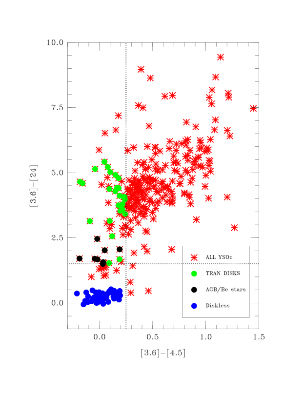
Figure 1: Color-color diagram illustrating our key target selection criteria. Objects with [3.6]-[4.5] $<$ 0.25 and [3.6] -[24] $<$ 0.5 are consistent with bare stellar photospheres. Blue dots are disk-less WTTSs from Cieza et al. (2007) used to define this region of the diagram. Red stars are all the 297 Young Stellar Objects Candidates (YSOc) in the Cores to Disks catalog of Ophiuchus. Most PMS stars are either disk-less or have excesses at both 4.5 and 24 $\mu$m. Our 26 transition disks, shown as green dots, have significant ($>$ 5-$\sigma$) excess at 24 $\mu$m and little or no excess at 4.5 $\mu$m, as expected for disks with inner holes. The 8 black dots are likely Be and AGB stars contaminating our original sample.

a. Have Spitzer colors [3.6]-[4.5] $<$ 0.25. These YSOc are objects with small or no near-IR excess (see Figure 1). The lack of a [3.6] - [4.5] color excess in our targets is inconsistent with an optically thick disk extending inward to the dust sublimation radius, and therefore indicates the presence of an inner opacity hole. The presence of this inner opacity hole is the defining feature we intend to capture in our sample. This feature is present in $\sim$21$\%$ of the YSOc in Ophiuchus as our first criterion selects 63 of them (out of 297).

b. Have Spitzer colors [3.6]-[24] $>$ 1.5. We apply this criterion to ensure all our targets have very significant excesses. It removes the 10 YSOc with smallest 24 $\micron$ excess (i.e., 1.5 $>$ [3.6]-[24] $>$ 1.0) and leaves 53 targets.

c. Are detected with signal to noise ratio $>$ 7 in all 2MASS and IRAC wavelengths as well as at 24 $\mu$m, to ensure we only include targets with very reliable photometry. This criterion removes 9 objects and leaves 44 targets.

d. Have K_S $<$ 11 mag , driven by the sensitivity of our near-IR adaptive optics observations and to ensure a negligible extragalactic contamination (Padgett et al. 2008). This criterion removes 6 objects and leaves 38 targets.

e. Are brighter than R = 18 mag according to the USNO-B1 catalog (Monet et al. 2003), driven by the sensitivity of our optical spectroscopy observations. This criterion removes 4 objects and leaves a final target list of 34 YSOc.

The first two selection criteria ( [3.6]-[4.5] $<$ 0.25 and [3.6]-[24] $>$ 1.5 ) effectively become our working definition for a transition disk. These criteria are fairly inclusive and encompass most of the transition disk definitions discussed in § 1 as they select disks with a significant flux decrement relative to “full disks” in the near-IR or at all wavelengths. Many of our targets have IR excesses that only become evident at 24 $\mu$m (see § 5.1.3). To check the reality of these excesses, we have visually inspected the cutouts of the 24 $\mu$m Ophiuchus mosaic created by the Cores to Disks project to confirm they show bona fide detections of our targets. We have also verified that all the 24 $\mu$m images of our targets have been assigned an “Image Type” = 1 in the Cores to Disks catalogs, corresponding to objects that are well fitted by a point source profile. As a final check, we have verified that all our targets have “well behaved” SEDs that are consistent with reddened stellar photospheres shortward of 4.5 $\mu$m and IR excesses from a disk at longer wavelengths. We have observed all 34 YSOc in our target list. However, as discussed in § 4.1.2, this list includes one likely classical Be star and 7 likely Asymptotic Giant Branch stars. The remaining 26 targets are bona fide PMS stars with circumstellar disks and constitute our science sample. The Spitzer and alternative names names, 2MASS and Spitzer fluxes, and the USNO-B1 R-band magnitudes for all our 34 targets are listed in Table 1.

3 Observations

3.1 Millimeter Wavelength Photometry

Two of our 34 targets, #14 and 17, have already been detected at millimeter wavelength (Andrews & Williams, 2007 ), while stringent upper limits exist for 3 others, #12, 13, and 27 (Cieza et al. 2008). We have observed 24 of the 29 remaining objects with the Submillimeter Array (SMA; Ho et al. 2004), and 5 of them with Bolocam at the Caltech Submillimeter Observatory (CSO). In § 4.2, we use the millimeter wavelength photometry to constrain the masses of our transition disks.

3.1.1 Submillimeter Array Observations

Millimeter interferometric observations of 24 of our targets were conducted in service mode with the SMA, on Mauna Kea, Hawaii, during the Spring and Summer of 2009 (April 6^th through July 16^th) in the compact-north configuration and with the 230 GHz/1300 $\mu$m receiver. Both the upper and lower sideband data were used, resulting in a total bandwidth of 4 GHz.

Typical zenith opacities during our observations were $\tau_{225\,{\rm GHz}}$ $\sim$0.15–0.25. For each target, the observations cycled between the target and two gain calibrators, 1625-254 and 1626-298, with 20-30 minutes on target and 7.5 minutes on each calibrator. The raw visibility data were calibrated with the MIR reduction package. The passband was flattened using $\sim$1 hour scans of 3c454.3 and the solutions for the antenna-based complex gains were obtained using the primary calibrator 1625-254. These gains, applied to our secondary calibrator, 1626-298, served as a consistency check for the solutions.

The absolute flux scale was determined through observations of either Callisto or Ceres and is estimated to be accurate to 15$\%$. The flux densities of detected sources were measured by fitting a point source model to the visibility data, while upper limits were derived from the rms of the visibility amplitudes. The rms noise of our SMA observations range from 1.5 to 5 mJy per beam. We detected, at the 3–$\sigma$ level or better, 5 of our 24 SMA targets: #3, 15, 18, 21, and 32. The 1.3 mm fluxes (and 3-sigma upper limits) for our entire SMA sample are listed in Table 2.

3.1.2 CSO-Bolocam Observations

Millimeter wavelength observations of 5 of our targets were made with Bolocam at the CSO on Mauna Kea, Hawaii, during June 25^th-30^th, 2009. The observations were performed in the 1.1 mm mode, which has a bandwidth of 45 GHz centered at 268 GHz. Our sources were scanned using a Lissajous pattern providing 10 min of integration time per scan. Between 16 and 40 scans per source were obtained. The weather was clear for the run, with $\tau_{225\,{\rm GHz}}$ ranging from 0.05 to 0.1. Several quasars close to the science fields were used as poniting calibrators, while Uranus and Neptune were used as flux calibrators. The data were reduced and the maps from individual scans were coadded using the Bolocam analysis pipeline , which consists of a series of modular IDL routines. None of the 5 targets were detected by Bolocam in the coadded maps, which have rms noises ranging from 3 to 6 mJy per beam. The 3-$\sigma$ upper limits for the 1.1 mm fluxes of our Bolocam targets are listed in Table 2.

3.2 Optical Spectroscopy

We obtained Echelle spectroscopy (resolution $>$ 20,000) for our entire sample using 3 different telescopes, Clay, CFHT, and Du Pont. All the spectra include the H$\alpha$ line, which we use to derive accretion rates (see § 4.3).

3.2.1 Clay–Mike Observations

We observed 14 of our targets with the Magellan Inamori Kyocera Echelle (MIKE) spectrograph on the 6.5-m Clay telescope at Las Campanas Observatory, Chile. The observations were performed in visitor mode on April 27^th and 28^th, 2009. We used the red arm of the spectrograph and a 1^′′ slit to obtain complete optical spectra between 4900 and 9500 Å at a resolution of 22,000. This resolution corresponds to $\sim$0.3 Å at the location of the H$\alpha$ line and to a velocity dispersion of $\sim$14 km/s. Since the CCD of MIKE’s red arm has a pixel scale of 0.05 Å/pixel, we binned the detector by a factor of 3 in the dispersion direction and a factor of 2 in the spatial direction in order to reduce the readout time and noise. The R-band magnitudes of our MIKE targets range from 15.5 to 18. For each object, we obtained a set of 3 or 4 spectra, with exposure times ranging from 3 to 10 minutes each, depending of the brightness of the targets. The data were reduced using the standard IRAF packages IMRED:CDDRED and ECHELLE:DOECSLIT.

3.2.2 CFHT–Espadons Observations

Twelve of our targets were observed with the ESPaDonS Echelle spectrograph on the 3.5-m Canada-France-Hawaii Telescope (CFHT) at Mauna Kea Observatory. The observations were performed in service mode during the last ESPaDonS observing run of the 2009A semester (June 30^th-July 13^th). The spectra were obtained in the standard “star+sky” mode, which delivers the complete optical spectra between 3500 Å and 10500 Å  at a resolution of 68,000, or 4.4 km/s. The R-band magnitudes of our ESPaDonS targets range between 7 and 15. For each object, we obtained a set of 3 spectra with exposures times ranging from 2.5 to 10 minutes each, depending on the brightness of the target. The data were reduced through the standard CFHT pipeline Upena, which is based on the reduction package Libre-ESpRIT.

3.2.3 Du Pont–Echelle Observations

We observed 8 of our targets with the Echelle Spectrograph on the 2.5-m Irenee du Pont telescope at las Campans Observatory. The observations were performed in visitor mode between May 14^th and May 16^th, 2009. We used a 1^′′ slit to obtain spectra between 4000 and 9000 Å  with a resolution of 45,000, corresponding to 0.14 Å in the red. However, since the Spectrograph’s CCD has a pixel scale of $\sim$0.1 Å/pixel, the true two-pixel resolution corresponds to $\sim$32,000, or $\sim$9.4 km/s in the red. The R-band magnitudes of our Du Pont targets range between 15.0 and 16.5. For each object, we obtained a set of 3 to 4 spectra with exposures times ranging from 10 to 15 minutes each, depending on the brightness of the target. The data reduction was performed using the standard IRAF packages IMRED:CDDRED and TWODSPEC:APEXTRACT.

3.3 Adaptive Optics Imaging

High spatial resolution near-IR observations of our entire sample were obtained with the Nasmyth Adaptive Optics Systems (NAOS) and the CONICA camera at the 8.2 m telescope Yepun, which is part the European Southern Observatory’s (ESO) Very Large Telescope (VLT) in Cerro Paranal, Chile. The data were acquired in service mode during the ESO’s observing period 84 (April 1^st through September 30^th, 2009).

To take advantage of the near-IR brightness of our targets, we used the infrared wavefront sensor and the N90C10 dichroic to direct 90$\%$ of the near-IR light to adaptive optics systems and 10$\%$ of the light to the science camera. We used the S13 camera (13.3 mas/pixel and 14$\times$14^′′ field of view) and the Double RdRstRd readout mode. The observations were performed through the K_s and J-band filters at 5 dithered positions per filter. The total exposures times ranged from 1 to 50 s for the K_S-band observations and from 2 to 200 s for the J-band observations, depending on the brightness of the target. The data were reduced using the Jitter software, which is part of ESO’s data reduction package Eclipse. In § 4.4, we use these Adaptive Optics (AO) data to constraint the multiplicity of our targets.

4 Results

4.1 Stellar properties

Before discussing the circumstellar properties of our targets, which is the main focus of our paper, we investigate their stellar properties. In this section, we derive their spectral types and identify any background objects that might be contaminating our sample of PMS stars with IR excesses.

4.1.1 Spectral Types

We estimate the spectral types of our targets by comparing temperature sensitive features in our echelle spectra to those in templates from stellar libraries. We use the libraries presented by Soubiran et al. (1998) and Montes (1998). The former has a spectral resolution of 42,000 and covers the entire 4500 – 6800 Å spectral range. The Latter has a resolution of 12,000 and covers the 4000 – 9000 Å spectral range with some gaps in the coverage. Before performing the comparison, we normalize all the spectra and take the template and target to a common resolution.

Most of our sources are M-type stars, for which we assign spectral types based on the strength of the TiO bands centered around 6300, 6700, 7150, and 7800 Å. We classify G-K stars based on the ratio of the V I (at 6199 Å) to Fe I (6200 Å) line (Padgett, 1996) and/or on the strength of the Ca I ( 6112 A) and Na I (5890 and 5896 Å) absorption lines (Montes et al. 1999; Wilking et al. 2005). There is also a B-type star in our sample, which we identify and type by the width of the underlying H$\alpha$ absorption line (which is much wider than its emission line) and by the strength of the Paschen 16, 15, 14, and 13 lines. The spectral types so derived are listed in Table 2. We estimate the typical uncertainties in our spectral classification to be 1 spectral subclass for M-type stars and 2 spectral subclasses for K and earlier type stars.

4.1.2 Pre-main-sequence stars identification

Background objects are known to contaminate samples of Spitzer-selected YSO candidates (Harvey et al. 2007, Oliveira et al. 2009). At low flux levels, background galaxies are the main source of contamination. However, the optical and near-IR flux cuts we have implemented as part of our sample selection criteria seem to have very efficiently removed any extragalactic sources that could remain in the Cores to Disks catalog of Ophiuchus YSO candidates. At the bright end of the flux distribution, Asymptotic Giant Branch (AGB) stars and classical Be stars are the main source of contamination. AGB stars are surrounded by shells of dust and thus have small, but detectable, IR excesses. The extreme luminosites ($\sim$10⁴ L_⊙) of AGB stars imply that they can pass our optical and near-IR flux cuts even if they are located several kpc away. Classical Be stars are surrounded by a gaseous circumstellar disk that is not related to the primordial accretion stage but to the rapid rotation of the object (Porter $\&$ Rivinius, 2003). Classical Be stars exhibit both IR excess (from free-free emission) and H$\alpha$ emission (from the recombination of the ionized hydrogen in the disk) and thus can easily be confused with Herbig Ae/Be stars (early-type PMS stars).

There is only one B-type star in our target list, object $\#$ 2. This object is located close to the eastern edge of the Cores to Disks maps of Ophiuchus, shows very little 24 $\mu$m excess, and is not detected at 70 $\mu$m. Its weak IR excess is more consistent with the free-free emission of a classical Be star than with the thermal IR excess produced by circumstellar dust around a Herbig Ae/Be star. Since there is no clear evidence that object $\#$ 2 is in fact a pre-main-sequence star, we do not include it in our sample of transition disks.

G and later type PMS stars can be distinguished from AGB stars by the presence of emission lines associated with chromospheric activity and/or accretion. H$\alpha$ (6562 Å) and the Ca II infrared triplet (8498, 8542, 8662 Å) are the most conspicuous of such lines. The Li I 6707 Å absorption line is also a very good indicator of stellar youth in mid-K to M-type stars because Li is burned very efficiently in the convective interiors of low-mass stars and is depleted soon after these objects arrive on the main-sequence. In Table 2, we tabulate the velocity dispersion of the H$\alpha$ emission lines, the equivalent widths of the detected Li I 6707 Å absorption lines, and the identification of the Ca II infrared triplets. After removing the Be star from consideration, we detect H$\alpha$ emission in 25 of our targets. All of them exhibit Li I absorption and/or Ca II emission and can therefore be considered bona fide PMS stars. Six of the targets exhibit H$\alpha$ absorption. All of them are M-type stars with small 24 $\mu$m excesses and no evidence for Li I absorption nor Ca II emission. Since these targets are most likely background AGB stars, we do not include them in our sample of transition disks. Two of our targets, objects # 12 and 22, show no evidence for H$\alpha$ emission or absorption. Object #12 is the well studied K-type PMS star Do Ar 21, and we thus include it in our transition disks sample. Object # 22 is a M6 star with small 24 $\mu$m excesses and no evidence for Li I absorption nor Ca II emission and is also a likely AGB star.

To sum up, after removing one classical Be star (object # 2) and seven likely AGB stars (objects # 4, 6, 8, 10, 22, 33, 34), we are left with 26 bona-fide PMS stars. These 26 objects constitute our sample of transition disks. As shown in Figure 1, all the contaminating objects have [3.6]-[24] $\lesssim$ 2.5, while 24 of the 26 PMS stars have [3.6]-[24] $\gtrsim$ 2.5. This result underscores the need for spectroscopic diagnostics to firmly establish the PMS sequence status of Spitzer-selected YSO candidates, especially those with small IR excesses.

4.2 Disk Masses

As shown by Andrews $\&$ Williams (2005,2007), disk masses obtained from modeling the IR and (sub)-mm SEDs of circumstellar disks are well described by a simple linear relation between (sub)-mm flux and disk mass. From the ratios of model-derived disk masses to observed mm fluxes presented by Andrews $\&$ Williams (2005) for 33 Taurus stars, Cieza et al. (2008) obtained the following relation, which we adopt to estimate the disk masses of our transition disks:

$$M_{DISK}=1.7\times 10^{-1}[(\frac{F_{\nu}(1.3mm)}{mJy})\times(\frac{d}{140pc})^{2}]M_{JUP}$$ (1)

Based on the standard deviation in the ratios of the model-derived masses to observed mm fluxes, the above relation gives disk masses that are within a factor of $\sim$2 of model-derived values; nevertheless, larger systematic errors can not be ruled out (see Andrews $\&$ Williams, 2007). In particular, the models from Andrews $\&$ Williams (2005, 2007) assume an opacity as a function of frequency of the form $K_{\nu}$ $\propto$ $\nu$ and a normalization of $K_{0}$ = 0.1 gr/cm² at 1000 GHz. This opacity implicitly assumes a gas to dust mass ratio of 100. Both the opacity function and the gas to dust mass ratio are uncertain and expected to change due to disk evolution processes such as grain growth and photoevaporation. Detailed modeling and a additional observational constraints on the grain size distributions and the gas to dust ratios will be needed to derive more accurate disk masses for each individual transition disk.

Since in the (sub)mm regime disk fluxes behave as $F_{\nu}\propto\nu^{2\pm 0.5}$ (Andrews $\&$ Williams, 2005), our targets are expected to be brighter (by a factor of $\sim$1.4) at 1.1 mm than they are at 1.3 mm. We thus modify Equation 1 accordingly to derive upper limits for the disk masses of the objects observed at 1.1 mm with the CSO. The disk masses (and 3-$\sigma$ upper limits) for our sample, derived adopting a distance to Ophiuchus of 125 pc (Loinard et al. 2008), are listed in Table 3. For two objects, #12 and 27, we adopt the disk mass upper limits from Cieza et al. (2008), which were derived from 850 $\mu$m observations. The vast majority of our transition disks have estimated disk masses lower than $\sim$2.0 M_JUP. However, two of them have disk masses typical of CTTSs ($\sim$3-5 M_JUP) and two others have significantly more massive disks ($\sim$10-40 M_JUP).

4.3 Accretion Rates

Most PMS stars show H$\alpha$ emission, either from chromospheric activity or accretion. Non-accreting objects show narrow ($<$ 200 km/s) and symmetric line profiles of chromspheric origin, while accreting objects present broad ($>$ 300 km/s) and asymmetric profiles produced by large-velocity magnetospheric accretion columns. The velocity dispersions (at 10 $\%$ of the peak intensity), $\Delta V$, of the H$\alpha$ emission lines of our transition disks are listed in Table 2. The boundary between accreting and non-accreting objects has been empirically placed by different studies at $\Delta V$ between 200 km/s (Jayawardana et al. 2003) and 270 km/s (White $\&$ Basri, 2003). Since only one of our objects, source # 25, has $\Delta V$ in the 200-300 km/s range, most accreting and non-accreting objects are clearly separated in our sample. Source # 25 has $\Delta V$ $\sim$230 km/s and a very noisy spectrum. We consider it to be non-accreting because it has a very low fractional disk luminosity (L_D/L_∗ $<$ 10^-3, see § 5.1.3).

The continuum-subtracted H$\alpha$ profiles for all the 17 accreting transition disks are shown in Figure 2, while those for the 8 non-accreting disks where the H$\alpha$ line was detected are shown in Figure 3. For accreting objects, the velocity dispersion of the H$\alpha$ line correlates well with accretion rates derived from detailed models of the magnetospheric accretion process. We therefore estimate the accretion rates of our targets from the width of the H$\alpha$ line measured at 10$\%$ of its peak intensity, adopting the relation given by Natta et al. (2004):

$$Log(M_{acc}(M_{\odot}/yr))=-12.89(\pm 0.3)+9.7(\pm 0.7)\times 10^{-3}\Delta V(km/s)$$ (2)

This relation is valid for 600 km/s $>$ $\Delta V$ $>$ 200 km/s (corresponding to 10^-7 M_⊙/yr $>$ M_acc 10^-11 M_⊙/yr) and can be applied to objects with a range of stellar (and sub-stellar) masses. The broadening of the the H${\alpha}$ line is 1 to 2 orders of magnitude more sensitive to the presence of low accretion rates than other accretion indicators such as U-band excess and continuum veiling measurements (Muzerolle et al. 2003, Sicilia-Aguilar et al. (2006b), and is thus particularly useful to distinguish weakly accreting from non-accreting objects. However, as discussed by Nguyen et al. (2009), the 10$\%$ width measurements are also dependent on the line profile, rendering the 10$\%$ H$\alpha$ velocity width a relatively poor quantitive accretion indicator, specially at high accretion rates (Muzerolle et al. 1998).

For the 9 objects we consider to be non-accreting, we adopt a mass accretion upper limit of 10^-11M_⊙/yr, corresponding to $\Delta V$ = 200 km/s. The so derived accretion rates (and upper limits) for our sample of transition disks are listed in Table 3. Given the large uncertainties associated with Equation 2 and the intrinsic variability of accretion in PMS stars, these accretion rates should be considered order-of-magnitude estimates.

4.4 Stellar companions

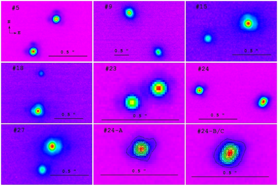
Figure 4: The K-band images of the seven multiple systems that have been detected with our VLT-AO observations. Target #24 is a triple system. The tighter components (#24-B and #24-C) are not fully resolved, but they presence can be inferred from the highly elongated image less than 1^′′ away from the perfectly round PSF of the source #24-A

Seven binary systems were identified in our sample by visual inspection of the VLT-AO images: targets #5, 9, 15, 18, 23, 24, and 27 (Figure 4). The separation and flux ratios of these systems range from 0.19^′′ to 1.68^′′ and 1.0 to 12, respectively. All these systems were well resolved in both our J- and K_S-band images, which have typical FWHM values of 0.06^′′-0.07^′′. Targets #9, 15, 18, and 27 are previously known binaries (Ratzka et al. 2005; Close et al. 2007), while targets #5, 23, and 24 are newly identified multiple systems. For each one of these binary systems, we searched for additional tight companions by comparing each other’s PSFs. The PSF pairs were virtually identical in all cases, except for target #24. The north-west component of this target has a perfectly round PSF, while the south-east component, 0.84^′′ away, is clearly elongated. Since variations in the PSF shape are not expected within such small angular distances and this behavior is seen in both the J- and K_s-band images, we conclude that target #24 is a triple system. We use the PSF of the wide component (object #24-A) to model the image of the tight components (object #24-B/C). We find that the image of the tight components is well reproduced by two equal-brightness objects 4 pixels apart (corresponding to $\sim$0.05^′′ or 6.6 AU) at a position angle of $\sim$30 deg.

We have also searched in the literature for additional companions in our sample that our VLT observations could have missed. In addition to the seven multiple systems discussed above, we find that source # 12 (Do Ar 21) is a binary system with a projected separation of just 0.005$"$ (corresponding to 0.62 AU), recently identified by the Very Long Baseline Array (Loinard et al. 2008). We also find that source # 27 is in fact a triple system. The “primary” star in the VLT observations is itself a spectroscopic binary with a 35.9 d period and an estimated separation of 0.27 AU (Mathieu et al. 1994). Additional multiplicity constraints exists for 2 other of our targets. Target #21 has been observed with the lunar occultation technique (Simon et al. 1995) and a similar-brightess companion can be ruled out down to $\sim$1 AU. Similarly, target #13 has been found to have a constant radial velocity ( $\sigma_{vel}<$ 0.25 km/s) during a 3 yr observing campaign (Prato, 2007).

For the apparently single stars, we estimated the detection limits at 0.1^′′ separation from the 5-$\sigma$ noise of PSF-subtracted images. For these objects, however, there are no comparison PSF’s available to perform the subtraction. Instead, we subtract a PSF constructed by azimuthally smoothing the image of the target itself, as follows. For each pixel in the image, the separation from the target’s centroid is calculated, with sub-pixel accuracy. The median intensity at that separation, but within an arc of 30 pixels in length, is then subtracted from the target pixel. Thus, any large scale, radially symmetric structures are removed. The detection limits at 0.1^′′ separation, obtained as described above, range from 2.4 to 3.5 mag, with a median value of 3.1 mag (corresponding to a flux ratio of 17). The separations, positions angles, and flux ratios of the multiple systems in our sample are shown in Table 2, together with the flux ratio limits of companions for the targets that appear to be single.

5 Discussion

5.1 Sample properties

In this section, we investigate the properties of transition disks as a group of objects. We discuss the properties of our targets (disk masses, accretion rates, multiplicity, SED morphologies, and fractional disk luminosities) and compare them to those of non-transition disks in order to place our sample into a broader context of disk evolution.

5.1.1 Disk Masses and Accretion Rates

To compare the disk masses and accretion rates of our sample of transition disks to those of non-transition disks, we collected such data from the literature for Ophichus objects with Spitzer colors [3.6]-[4.5] $>$ 0.25 and [3.6]-[24] $>$ 1.5. These are objects that have both near-IR and mid-IR excesses and therefore are likely to have “full disks”, extending inward to the dust sublimation radius. We collected disk masses for non-transition disks from Andrews $\&$ Williams (2007). This comparison sample is appropriate because our mm flux to disk mass relation (i.e., Equation 1) has been calibrated using their disk models. The accretion rates for our comparison sample come from Natta et. (2006), and have been calculated from the luminosity of the Pa$\beta$ line. This comparison sample is also appropriate because the relations between the luminosity of the Pa$\beta$ line and accretion rate and between the H$\alpha$ full width at 10$\%$ intensity and accretion rate (which we use for our transition disk sample) have both been calibrated by Natta et al. (2004) using the same detailed models of magnethospheric accretion.

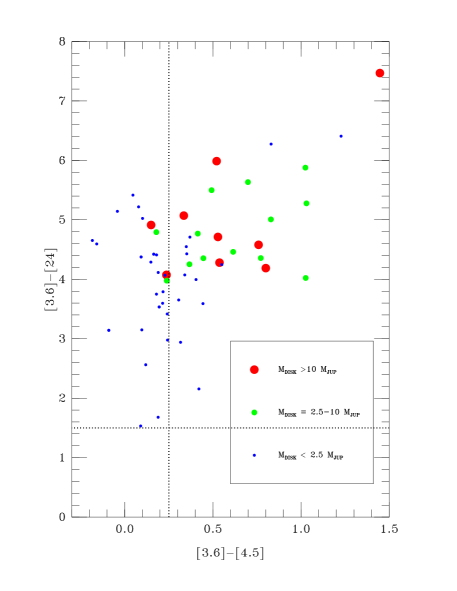
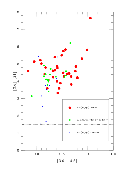
Figure 5: The [3.6] -[24] vs [3.6]-[4.5] colors of Ophiuchus PMS stars with disks of different masses (left) and accretion rates (right). Transition disks (in the left side of the figure, with [3.6]-[4.5] $<$ 0.25 ) tend to have much lower disk masses and accretion rates than non-transition objects. The disk masses of non-transition disk sample have been taken from Andrews $\&$ Williams (2007). The accretion rates of non-transition disks have been taken from Natta et al. (2006).

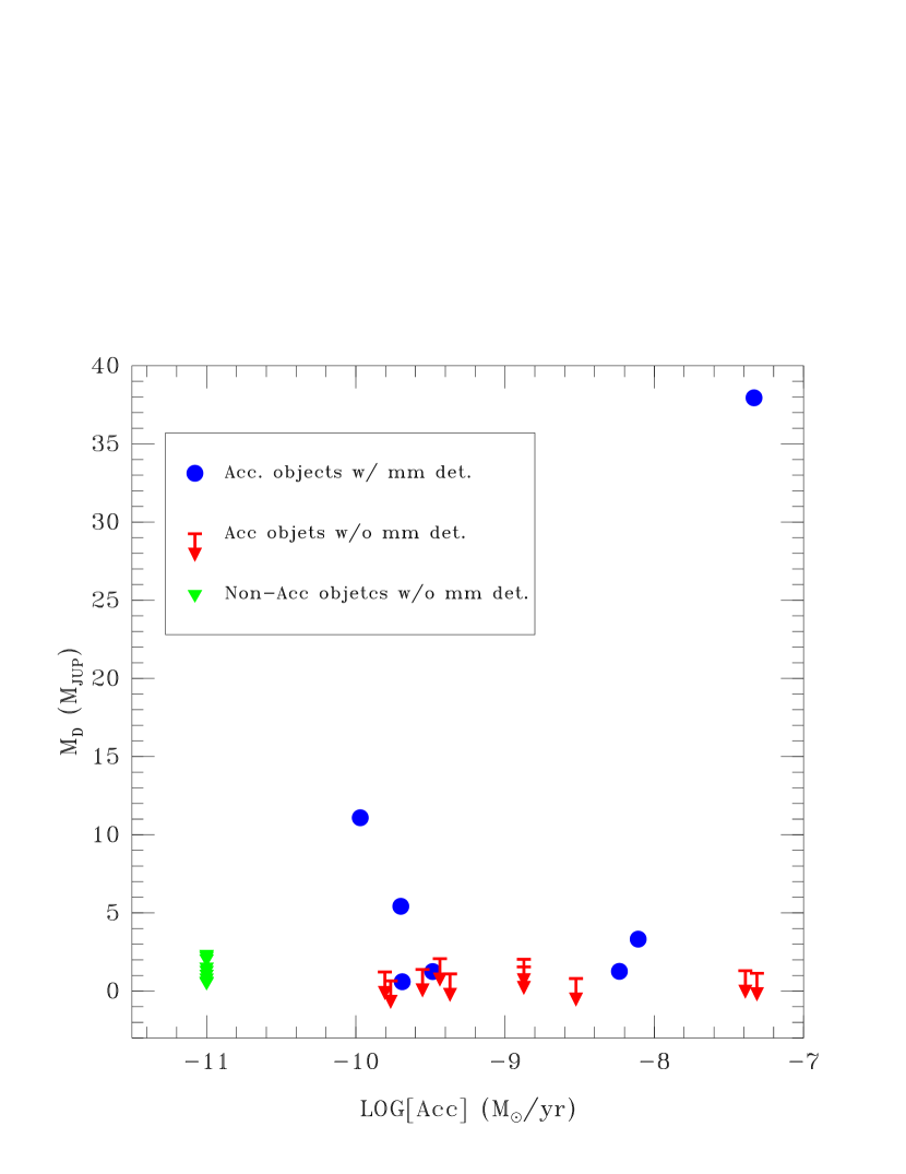
Figure 6: Disk masses vs. accretion rates for accreting objects with mm detections (blue circles), accreting objects with mm upper limits (red arrows), and non-accreting objects with mm upper limits (green triangles). None of the non-accreting objects was detected at mm wavelength.

Figure 5 shows that transition disks tend to have much lower disk masses and accretion rates than non-transition objects. We also find a strong connection between the magnitude of the mid-IR excess and both disk mass and accretion rate: objects with little ($\lesssim$ 4 mag) 24 $\mu$m excess tend to have small disk masses and low accretion rates. Among our transition disk sample, we also note that all of the mm detections correspond to accreting objects and that even some of the strongest accretors have very low disk masses (see Figure 6). In other words, massive disks are the most likely to accrete, but some low-mass disks can also be strong accretors.

These results can help reconcile the apparently contradictory findings of previous studies of transition disks. As discussed in § 1, Najita et al. (2007) studied a sample of 12 transition objects in Taurus and found that they have a median disk mass of 25 M_JUP, which is $\sim$4 times larger than the rest of the disks in Taurus, while Cieza et al. (2008) found that the vast majority of their 26 transition disk targets had very small ($<$ 2 M_JUP) disk masses. Our results now show that transition disks are a highly heterogeneous group of objects, whose “mean properties” are highly dependent on the details of the sample selection criteria. On the one hand, the sample studied by Cieza et al. (2008) was dominated by weak-line T Tauri stars. This explains the low disk masses they found, as lack of accretion is a particularly good indicator of a low disk mass (See Figure 6). One the other hand, Najita et al. (2006) drew their sample from the Spitzer spectroscopic survey of Taurus presented by Furlan et al. (2006), which in turn selected their sample based on mid-IR colors and fluxes from the Infrared Astronomical Satellite (IRAS). As a result, the Spitzer spectroscopic survey of Taurus was clearly biased towards the brightest objects in the mid-IR. This helps to explain the high disk masses obtained for the transition disks studied by Najita et al. (2006), as objects with strong mid-IR excesses tend to have higher disk masses (Figure 5).

5.1.2 Multiplicity

As discussed in § 1, dynamical interactions between the disk and stellar companion is one of the main mechanisms proposed to account for the opacity holes of transition disks. However, the fraction of transition disks that are in fact close binaries still remains to be established. If binaries play a dominant role in transition disks, one would expect a higher incidence of close binaries in transition disks that in non-transition disks. In order to test this hypothesis, we compare the distribution of binary separations of our sample of transition disk to that of non-transition disk (and disk-less PMS stars). We drew our sample of non-transition disks and disk-less PMS stars from the compilation of Ophiuchus binaries presented by Cieza et al. (2009).

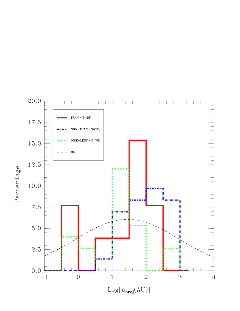
Figure 7: Distribution of companion separations for our transition disk sample (red dashed line), non-transition disks (blue dash-doted line), and disk-less stars (green dotted line). Spectroscopic binaries have been assigned a projected separation of 0.5 AU. The total number of objects (i.e., single + multiple systems) in each sample are shown in parenthesis. The distribution of binary separations for main sequence (MS) solar-type stars (Duquennoy $\&$ Mayor, 1991) is shown for comparison.

As shown by Figure 7, disk-less PMS stars tend to have companions at smaller separations than stars with regular, non-transition disks. According to a two-sided Kolmogoro–Smirnov (KS) test, there is only a 0.5$\%$ probability that the distributions of binary separations of non-transition disks and disk-less stars have been drawn from the same parent population. As discussed by Cieza et al. (2009), this result can be understood in terms of the effect binaries have on circumstellar disks lifetimes via the tidal truncation of the outer disk. For instance, a binary system with a 30 AU separation is expected to initially have individual disks that are $\sim$10-15 AU in radius. Given that the viscous timescale is roughly proportional to the size of the disk, such small disks are likely to have very small accretion lifetimes, smaller than the age of the sample.

For systems with binary separations much smaller than the size of a typical disk, the outer disk can survive in the form of a circumbinary disk, with a tidally truncated inner hole with a radius $\sim$2$\times$ the orbital separation (Artymowicz $\&$ Lubow, 1994). Such systems could be classified as transition disks based on their SEDs. We do not see an increased incidence of binaries with separations in the $\sim$8-20 AU range, the range where we are sensitive to companions that could in principle carve the inferred inner holes. In fact, the incidence of binaries in this separation range is lower for our transition disks than it is for the samples of both non-transition disks and disk-less stars. This suggests that stellar companions at 8-20 AU separations are not responsible for a large fraction of the transition disk population. Given the size of our transition disk sample, however, this result carries little statistical weight, and should be considered only a hint. According to a KS test, the distribution of binaries separations of transition objects is indistinguishable from that of both non-transition disks (p = 28$\%$) and disk-less stars (p = 12$\%$). On the other hand, the fact that 2 of our transition disk targets have previously known companions at sub-AU separations suggests that circumbinary disks around very tight systems (e.g., r $\lesssim$ 1-5 AU) could indeed represent an important component of the transition disk population. Unfortunately, the presence of tight companions (r $\lesssim$ 8 AU) remains completely unconstrained for most of our sample. A complementary radial velocity survey to find the tightest companions is highly desirable to firmly establish the fraction of transition disks that could be accounted for by close binaries.

5.1.3 SED morphologies and fractional disk luminosities

In addition to the disk mass, accretion rate, and multiplicity, the SED morphology and fractional disk luminosity of a transition disk can provide important clues on the nature of the object. In this section, we quantify the SED morphologies and fractional disk luminosities of our transition objects in order to compare them to the values of objects with “full disks”.

The diversity of SED morphologies seen in transition disks can not be properly captured by the traditional classification scheme of young stellar objects (i.e., the class I through III system), which is based on the slope of the SED between 2 and 25 $\mu$m (Lada 1987). Instead, we quantify the SED “shape” of our targets adopting the two-parameter scheme introduced by Cieza et al. (2007), which is based on the longest wavelength at which the observed flux is dominated by the stellar photosphere, $\lambda_{turn-off}$, and the slope of the IR excess, $\alpha_{excess}$, computed as dlog($\lambda$F)/dlog($\lambda$) between $\lambda_{turn-off}$ and 24 $\mu$m. The $\lambda_{turn-off}$ and $\alpha_{excess}$ values for our entire sample are listed in Table 3.

The $\lambda_{turn-off}$ and $\alpha_{excess}$ parameters provide useful information on the structure of the disk. In particular, $\lambda_{turn-off}$ clearly correlates with the size of the inner hole as it depends on the temperature of the dust closest to the star. Wien’s displacement law implies that Spitzer’s 3.6, 4.5, 5.8, 8.0, and 24 $\mu$m bands best probe dust temperatures of roughly 780K, 620K, 480K, and 350K, and 120K, respectively. For stars of solar luminosity, these temperatures correspond to circumstellar distances of $\lesssim$1 AU for the IRAC bands and $\sim$10 AU for the 24 $\mu$m MIPS band. Similarly, $\alpha_{excess}$ correlates well with the sharpness of the hole: a sharp inner hole, such as that of CoKu Tau/4, is characterized by a large and positive $\alpha_{excess}$ value, while a continuous disk that has undergone significant grain growth and dust settling is characterized by a large negative $\alpha_{excess}$ value (Dullemond $\&$ Dominik, 2004). However, the $\lambda_{turn-off}$ and $\alpha_{excess}$ parameters should be interpreted with caution. Deriving accurate disk properties from a SED requires detailed modeling because other properties, such as stellar luminosity and disk inclination, can also affect the $\lambda_{turn-off}$ and $\alpha_{excess}$ values.

The fractional disk luminosity, the ratio of the disk luminosity to the stellar luminosity (L_D/L_∗), is another important quantity that relates to the evolutionary status of a disk. On the one hand, typical primordial disks around CTTSs have L_D/L_∗ $\sim$ 0.1 as they have optically thick disks that intercept (and reemit in the IR) $\sim$10$\%$ of the stellar radiation. On the other hand, debris disks show L_D/L_∗ values $\lesssim$ 10^-3 because they have optically thin disks that intercept and reprocess $\sim$10^-5–10^-3 of the star’s light (e.g., Bryden et al. 2006).

We estimate L_D/L_∗ for our sample of transition disks using the following procedure. First, we estimate L_∗ as in Cieza et al (2007), by integrating over the broad-band colors given by Kenyon $\&$ Hartmann (1995) for stars of the same spectral type as each one of the stars in our sample. The integrated fluxes were normalized to the J-band magnitudes corrected for extinction, adopting A_J =1.53 $\times$ E(J-K_S ), where E(J-K_S) is the observed color excess with respect to the expected photospheric color. Then, we estimated L_D by integrated the estimated disk fluxes, the observed fluxes (or upper limits) minus the contribution of stellar photosphere at each wavelength between $\lambda_{turn-off}$ and 1.3 mm (or 850 $\mu$m for targets #12 and 27). The disk was assumed to contribute 30$\%$ of the flux at $\lambda_{turn-off}$ (e.g., a small but non-negligible amount, consistent with our definition of $\lambda_{turn-off}$).

The near and mid-IR luminosities of our transition disks are well constrained because their SEDs are relatively well sampled at these wavelengths. However, their far-IR luminosities remain more poorly constrained. Only 9 of our 34 targets have ( 5-$\sigma$ or better) detections at 70 $\mu$m listed in the Cores to Disks catalog. For the rest of the objects, we have obtained 5-$\sigma$ upper limits, from the noise of the 70 $\mu$m images at the location of the targets, in order to fill the gap in their SEDs between 24 $\mu$m and the millimeter. In particular, we used 120^′′ $\times$ 120^′′ cut outs of the Ophichus mosaic created by the Cores to Disks project from the “filtered” Basic Calibrated Data. We calculated the noise as 1-$\sigma$ = 2$\times$1.7(rms_sky)$\sqrt{N}$, where rms_sky is the flux rms (in mJy) of an annulus centered on the source with an inner and outer radius of 40 and 64^′′, respectively. N is the number of (4^′′) pixels in a circular aperture of 16^′′ in radius, and 1.7 is the aperture correction appropriate for such sky annulus and aperture size . The factor of 2 accounts for the fact that the images we use have been resampled to pixels that are half the linear size of the original pixels, artificially reducing the noise of the images (by $\sqrt{\frac{N_{res}}{N_{orig}}}$, where N_res and N_orig are, respectively, the number of resampled and original pixels in the sky annulus).

The LOG(L_D/L_∗) values for our transition disk sample, ranging from -4.1 to -1.5 are listed in Table 3. As most of the luminosity of a disk extending inward to the dust sublimation temperature is emitted in the near-IR, L_D/L_∗ is a very strong function of $\lambda_{turn-off}$: the shorter the $\lambda_{turn-off}$ wavelength, the higher the fractional disk luminosity. For objects with $\lambda_{turn-off}$ $<$ 8.0 $\mu$m, the 70 $\mu$m flux represent only a minor contribution to the total disk luminosity. On the other hand, objects with with $\lambda_{turn-off}$ $=$ 8.0 $\mu$m (i.e., objects with significant excess at 24 $\mu$m only) have much lower L_D/L_∗ values, and the 70 $\mu$m emission becomes a much larger fraction of the total disk luminosity. As a result, the L_D/L_∗ values of objets with $\lambda_{turn-off}$ $=$ 8.0 $\mu$m and no 70 $\mu$m detections should be considered upper limits.

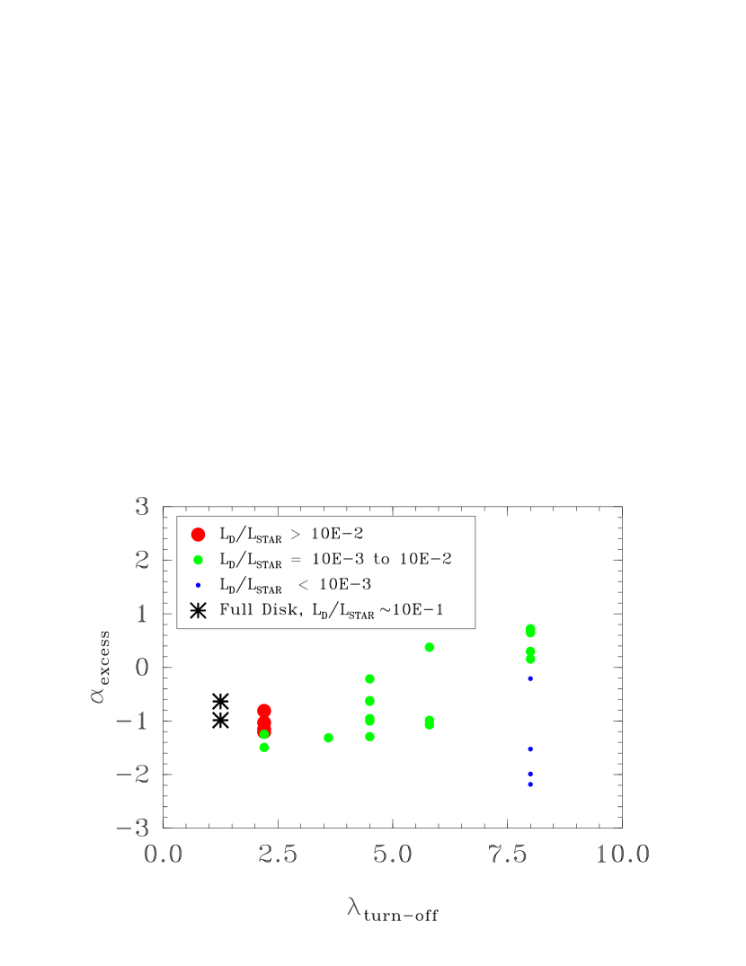
Figure 8: $\alpha_{excess}$ vs. $\lambda_{turn-off}$ for objects with different L_D/L_∗ values. The loci of “typical” CTTS with full disks are shown for comparison. Transition disks occupy a much larger parameter space

As shown in Figure 8, our transition disks span the range $\lambda_{turn-off}$ = 2.2 to 8.0 $\micron$ and $\alpha_{excess}$ $\sim$ -2.5 to 1, while typical CTTSs occupy a much more restricted region of the parameter space. Based on the median and quartile SEDs presented by Furlan et al (2006), 50$\%$ of late-type (K5–M2) CTTSs have $\lambda_{turn-off}$ = 1.25 $\micron$, -1.0 $>$ $\alpha_{excess}$ $>$ -0.64, and fractional disk luminosities in the 0.07 to 0.15 range. As discussed by Cieza et al. (2005), CTTS are likely to have J-band excesses. However, since this excess is at the $\lesssim$ 30-40$\%$ level, the observed J-band fluxes are still dominated by the stellar photospheres, satisfying our $\lambda_{turn-off}$ definition. Figure 8 also shows that, as expected, transition disks with different L_D/L_∗ values occupy different regions of the $\alpha_{excess}$ vs. $\lambda_{turn-off}$ space. Objects with L_D/L_∗ $>$ 10^-2 lay close to the CTTSs loci, while objects with L_D/L_∗ $<$ 10^-3 all have $\lambda_{turn-off}$ = 8.0 $\micron$ and $\alpha_{excess}$ $\lesssim$ 0.0. The objects in the latter group are all non-accreting. Their very low fractional disk luminosities and lack of accretion suggest they are already in a debris disk stage (see § 5.2.1).

5.2 The Origin of the Opacity Holes

The four different mechanisms that have been proposed to explain the inner holes of transition disks can be distinguished when disk masses, accretion rates and multiplicity information are available (Najita et al., 2007; Cieza, 2008; Alexander, 2008). In this section, we compare the properties of our transition disk sample to those expected for objects whose opacity holes have been produced by these four mechanisms: photoevaporation, tidal truncation in close binaries, grain-growth, and giant planet formation.

5.2.1 Photoevaporation

According to photoevaporation models (e.g., Alexander et al. 2006), extreme UV photons, originating in the stellar chromosphere, ionize and heat the circumstellar hydrogen. Beyond some critical radius, the thermal velocity of the ionized hydrogen exceeds its escape velocity and the material is lost as a wind. At early stages in the evolution of the disk, the accretion rate across the disk dominates over the evaporation rate, and the disk undergoes standard viscous evolution. Later on, as the accretion rate drops to the level of the photoevaporation rate, the outer disk is no longer able to resupply the inner disk with material, the inner disk drains on a viscous timescale, and an inner hole is formed. Once an inner hole has formed, the entire disk dissipates very rapidly from the inside out as a consequence of the direct irradiation of the disk’s inner edge. Thus, transition disks created by photoevaporation are expected to have relatively low masses (M_DISK $<$ $5M_{JUP}$) and negligible accretion ($<$10^-10 M_⊙yr^-1).

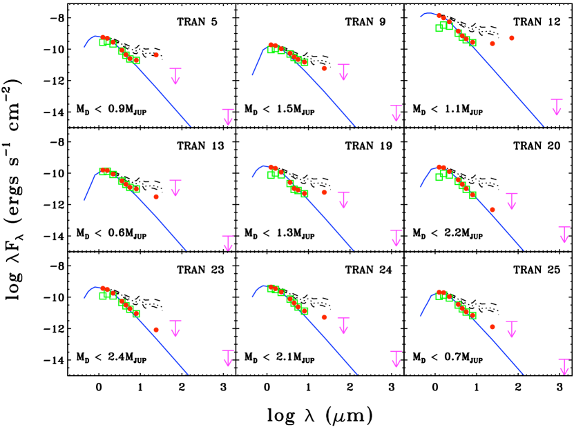
Figure 9: The SEDs of our non-accreting transition disk targets. All of them have low disk masses ($<$ 2.5 M_JUP), and are consistent with photoevaporation. The filled circles are detections while the arrows represent 3-$\sigma$ limits. The open squares correspond to the observed optical and near-IR fluxes before being corrected for extinction using the A_J values listed in Table 3 and the extinction curve provided by the Asiago database of photometric systems (Fiorucci $\&$ Munari 2003). For each object, the average of the two R-band magnitudes (from the USNO-B1 catalog) listed in Table 1 has been used. The solid blue line represent the stellar photosphere normalized to the extinction-corrected J-band. The dotted lines correspond to the median mid-IR SED of K5–M2 CTTSs calculated by Furlan et al. (2006). The dashed lines are the quartiles.

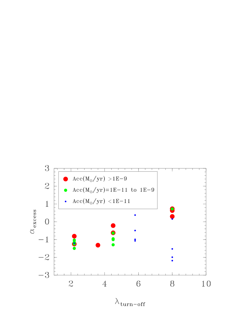
Figure 10: The $\alpha_{excess}$ (the slope of the IR excess) vs. $\lambda_{turn-off}$ (the wavelength at which the excess becomes significant) for our sample of transition disks. The masses and accretion rates are indicated by different symbols. The 4 accreting (targets #11, 2, 31, and 32) and the 2 non-accreting (targets #5 and 19) objects with $\alpha_{excess}~{}\gtrsim$ 0 are suggestive of sharp inner holes.

We find that 9 of our 26 transition disks have low disk mass ($<$ 0.6-2.5 M_JUP) and negligible accretion (M_acc $<$ 10^-11 M_⊙/year) and are hence consistent with photoevaporation. The SEDs of these objects are shown in Figure 9. These objects appear all in the lower left corner of Figure 6, which shows the disk mass as a function of accretion rate for our sample. However, they occupy different regions of the $\alpha_{excess}$ vs $\lambda_{turn-off}$ parameter space. The majority of these objects have $\alpha_{excess}$ $\lesssim$ -1, the typical value of CTTS with “full disks” (see Figure  10). These objects are therefore consistent with relatively flat, radially continuous disks. Two objects, targets # 5 and 19, have $\alpha_{excess}$ $\gtrsim$ 0, and are thus suggestive of sharp inner holes. Target #12 also has an steep SED, but between 24 and 70 $\mu$m, suggesting a larger inner hole . Sharp inner holes could also arise from dynamical interactions between the disk and large bodies within it. Photoevaporation and dynamical interactions are not mutually exclusive processes, as photoevaporation can also operate on a dynamically truncated disk as long as the disk mass and accretion rates are low enough. Coku Tau/4 is perhaps the most extreme example of this scenario. It is a 8 AU separation, equal-mass, binary system (Ireland & Kraus, 2008) resulting on a $\alpha_{excess}$ value of $\sim$2. Just like targets #5, 12, and 19, Coku Tau/4 lacks accretion and has a very low disk mass (Najita et al. 2007), and is consequently also susceptible to photoevaporation. Our VLT-AO observations reveal no stellar companion within $\sim$8 AU of targets #5, 12, or 19. However, target #12 is already known to be very tight binary (r $\lesssim$ 1 AU), and the presence of stellar (or planetary mass) companions remains completely unconstrained for targets #5 and 19.

Photoevaporation provides a natural mechanism for objects to transition from the primordial to the debris disk stage. Once accretion stops, photoevaporation is capable of removing the remaining gas in a very short ($<<1$ Myr) timescale (Alexander et al. 2006). As the gas in the disk photoevaporates, it is likely to carry with it the smallest grains present in the disk. What is left represents the initial conditions of a debris disk: a gas poor disk with large grains, planetesmals and/or planets. The very short photoevaporation timescale implies that some of the systems shown in Figure 9 could already be in a debris disk stage. In fact, the 4 non-accreting objects with L_D/L_∗ $<$ 10^-3 have properties that are indistinguishable from those of young debris disks like AU Mic and GJ 182 (Liu et al. 2004). These 4 objects are # 12, 20, 23, and 25. These objects might have already formed planets or might be in a multiple system (like target #12 is). Either way, most of the circumstellar gas and dust has already been depleted, and what we are currently observing could be the initial architectures of different debris systems, now subjected to processes such as dynamical interactions, the Poynting–Robertson effect and radiation pressure. The rest of the non accreting objects, #5, 9, 13, 19, and 24, have L_D/L_∗ $>$ 10^-3 and could be in the process of being photoevaporated.

5.2.2 Close binaries

Circumbinary disks are expected to be tidally truncated and have inner holes with a radius $\sim$2$\times$ the orbital separation (Artymowicz $\&$ Lubow, 1994). It is believed that most PMS stars are in multiple systems (Ratzka et al. 2005) with the same semi-major axis distribution as MS solar-type stars (e.g., a lognormal distribution centered at $\sim$28 AU). As a result, $\sim$30$\%$ of all Ophiuchus binaries are expected to have separations in the $\sim$1-20 AU range. If the primodial disk has survived in such systems, it is likely to be in the form of a circumbinary disk with tidally truncated inner holes up to 40 AU in radius. These close binary systems could hence be classified as transition disks based on their IR SEDs.

Four of our targets have companions close enough to suspect they could be responsible for the observed hole, namely sources # 12, 27, 24, and 23, in increasing order of projected separation. Source # 12 is a binary with a projected separation of $\sim$0.6 AU and $\lambda_{turn-off}$= 8.0 $\mu$m, which implies the disk must be a circumbinary one. However, given the long $\lambda_{turn-off}$ wavelength and tightness of the binary system, it seems unlikely that the present size of the inner hole is directly connected to the presence of the stellar companion. Source # 27 is triple system with projected separations of $\sim$0.3 AU and 41 AU and $\lambda_{turn-off}$ = 4.5 $\mu$m. The IR excess could originate at a circumbinary disk around the tight components of the system or at a circumstellar disk around the wide component. Target #24 is also a triple system with projected separations of $\sim$7 and 105 AU and $\lambda_{turn-off}$ = 5.8 $\mu$m. The IR excess could also in principle originate at a circumbinary disk around the tight components of the system. However, a circumprimary disk around source # 24-A is an equally likely possibility. Target # 23 is a $\sim$0.19^′′ (or 24 AU) separation binary with $\lambda_{turn-off}$ = 8.0 $\mu$m. This object has a small 24 $\mu$m excess, consistent with Wien side of the emission from a cold outer disk. Objects # 12 and 23 have a low disk masses ($<$ 1.7 M_JUP), negligible accretion, and L_D/L_∗ $<$ 10^-3. As discussed in the previous section, they are likely to be in the debris disk stage, regardless of the origin of the inner hole. After target #23, the next tighter binary is source #5, with a projected separation of 0.54^′′ (or 68 AU). Since this object has $\lambda_{turn-off}$ = 5.8 $\mu$m, suggesting the presence of dust at $\lesssim$1 AU distances, it is very unlikely that the presence of its inner hole is related to the observed companion. Since VLT-AO observations are clearly not sensitive to companions with separations $\lesssim$ 8 AU, a complementary radial velocity survey to find the tightest companions would be highly desirable to identify additional circumbinary disks within our sample.

5.2.3 Grain growth

Once primordial sub-micron dust grains grow into somewhat larger bodies (r _dust $\gg$ $\lambda_{stellar-photons}$), most of the solid mass ceases to interact with the stellar radiation, and the opacity function decreases dramatically. Grain growth is a strong function of radius; it is more efficient in the inner regions where the surface density is higher and the dynamical timescales are shorter, and hence can also produce opacity holes. Idealized dust coagulation models (i.e., ignoring fragmentation and radial drift) predict extremely efficient grain growth (Dullemond $\&$ Dominik, 2005) resulting in the depletion of all small grains in timescales of the order of 10⁵ yrs, which is clearly inconsistent with the observational constraints on the lifetime of circusmtellar dust. In reality, however, the persistence of small opacity-bearing grains depends on a complex balance between dust coagulation and fragmentation (Dominik $\&$ Dullemond, 2008).

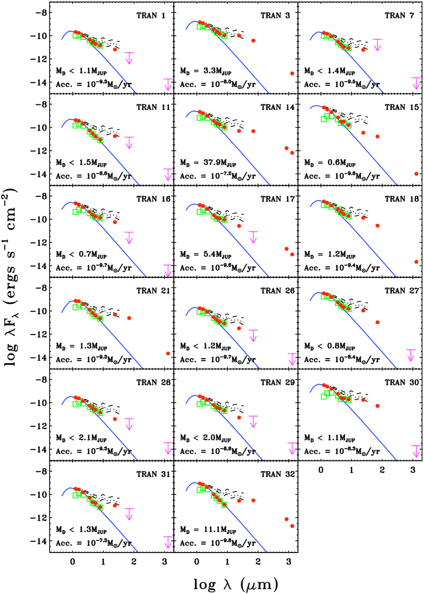
Figure 11: The SEDs of all our accreting transition disk targets. The symbols are the same as in Fig. 9. Disk masses range from $<$ 0.7 to $\sim$40 M_JUP. For targets # 14, 17, and 32, 850 $\mu$m fluxes, from Andrews $\&$ Williams (2007) and Nutter et al. (1996), are shown in addition to the 1.3 mm fluxes listed in Table 2.

Since grain growth affects only the dust and operates preferentially at smaller radii, a disk evolution dominated by grain growth is expected to result in an actively accreting disk with reduced opacity in the inner regions. All the accreting disks in our sample, whose SEDs are shown in Figure 11, are thus in principle consistent with grain growth. Objects with very strong accretion (i.e., $\gtrsim$ 10^-8 M_⊙yr^-1) are especially good candidates for grain growth dominated disks as an opacity hole is likely to trigger the onset of the magneto-rotational instability and exacerbate accretion (Chiang $\&$ Murray-Clay, 2007). Target #14, which is the extensively studied system DoAr 25, is a prime example of this scenario. It has, by far, the highest disk mass in our sample ($\sim$38 M_JUP) and one of the highest accretion rates ($\sim$10^-7.2 M_⊙yr^-1). This object has recently been imaged at high spatial resolution with the Submillimeter Array, and its SED and visibilities have been successfully reproduced with a simple model incorporating significant grain growth in its inner regions (Andrews et al. 2008).

Grain growth is considered the first step toward planet formation. Unfortunately, the observational effects of grains growing into terrestrial planets are no different from those of growing into meter size objects. As a result, the observations presented herein place no constraints on how far along the planet formation process currently is, unless the planet becomes a giant planet, massive enough to dynamically open a gap in the disk.

5.2.4 Giant planet formation

Since theoretical models of the dynamical interactions of forming giant planets with the disk (Lin $\&$ Papaloizous 1979, Artymowicz $\&$ Lubow 1994) predict the formation of inner holes and gaps, planet formation quickly became one of the most exciting explanations proposed for the inner holes of transition disks (Calvet et al. 2002, 2005; Quillen et al. 2004; D’Alessio et al. 2005; Brown et. 2008). A planet massive enough to open a gap in the disk (M $\gtrsim$0.1-0.5 M_JUP), is expected to divert most of the material accreting from the outer disk onto itself. As a result, in the presence of a Jupiter mass planet, the accretion onto the star is expected to be reduced by a factor of 4 to 10 with respect to the accretion across the outer disk (Lubow $\&$ D^′Angelo, 2006).

Four of the accreting objects in our sample, targets # 11, 21, 31, and 32 have $\alpha_{excess}$ $>$ 0, suggesting the presence of a sharp inner hole, and are thus excellent candidates for ongoing giant planet formation. Source #32 is a particularly good candidate to be currently forming a massive giant planet, as it has a high disk mass ($\sim$11 M_JUP) and small accretion rate (10^-9.8 M_⊙yr^-1). Sources #11, 21, and 31 (M_D $<$ 1.5 M${}_{JUP};$ M_acc $\sim$10^-9.3-10^-7.3 M_⊙yr^-1), could have formed a massive giant planet in the recent past, as in their case most of the disk mass has already been depleted. Since target #21 has been observed with the lunar occultation technique, an equal-mass binary system can be ruled out for this system down to $\sim$1 AU (Simon et al. 1995). Also, it has been proposed that companions with masses of the order of 10 M_JUP completely isolate the inner disk from the outer disk and halt the accretion onto the star (Lubow et al. 1999). If that is the case, accretion itself could be evidence against the presence of a close (sub)stellar companion. That said, because a few accreting close binary systems are already known, such as DQ Tau (Carr et al. 2001) and CS Cha (Espaillat et al. 2007), it is clear that accretion does not rule out completely the presence of tight stellar companions. In addition to the mass of the companion, the eccentricity of the orbit, the viscosity and scale height of the disk are also important factors in determining whether or not gap-crossing streams can exist and allow the accretion onto the star to continue (Artymowicz $\&$Lubow 1996).

5.2.5 Disk Classification

Based on the discussion above, we divide our transition disk sample into the following “disk types”:

a) 13 grain growth-dominated disks (accreting objects with $\alpha$ $\lesssim$ 0).
b) 4 giant planet forming disks (accreting objects with $\alpha$ $\gtrsim$ 0).
c) 5 photoevaporating disks (non-accreting objects with disk mass $<$ 2.5 M_JUP, but L_D/L_∗ $>$ 10^-3)
d) 4 debris disks (non-accreting objects with disk mass $<$ 2.5 M_JUP and L_D/L_∗ $<$ 10^-3)
e) 4 circumbinary disks (a binary tight enough to accommodate both components within the inferred inner hole).

The total number of objects listed add up to 30 instead of 26 because 4 objects fall into two categories. Sources # 12 and 23 are considered both debris disks and circumbinary disks. Object #24 has been classified as both a circumbinary disk and a photoevaporating disk, while object # 27 has been classified as both a circumbinary disk and a grain growth dominated disk. These last two objects are triple systems and their classification depends on whether the IR excess is associated with the tight components of the systems or with the wide components.

The “disk types” for our targets are listed in Table 3. All of our objects should be considered to be candidates for the categories listed above. The current classification represents our best guess given the available data. Only followup observations and detailed modeling will firmly establish the true nature of each object. An important caveat of this classification is the lack of constraints for most of the sample on stellar companions within $\lesssim$ 8 AU, a range where $\sim$30$\%$ of all stellar companions are expected to lay (Duquennoy $\&$ Mayor, 1991; Ratzka et al. 2005). Future radial velocity observations are very likely to increase the number of objects in the circumbinary disk category.

While it is tempting to speculate that the “disk types” a through d represent an evolutionary sequence, starting with a “full disk” (i.e., a “full disk” that undergoes grain growth followed by giant planet formation, followed by photoevaporation leading to a debris or disk-less stage) it is clear that not all disks follow this sequence. For instance, many of the grain growth dominated disks have disk masses that are 10 times smaller than some of the giant planet forming disks (e.g., targets #1, 15, 16, and 26 vs. #32). These former systems have very little mass left in the disk ($\lesssim$ 1 M_JUP) and might never form giant planets. It it also clear that not all disks become transition disks in the same way. Some objects become transition disks (as defined by their SEDs) while the total mass of the disk is very large (e.g., targets #32 and 14, M_D $\sim$10-40 M_JUP), but other objects retain “full disks” even when the disk mass is relatively small (M_D $\sim$2 M_JUP), such as ROXR1 29 (Cieza et al. 2008). Since very little dust is needed to keep a disk optically thick at near and mid-IR wavelengths, it is expected that some objects will only become transition disks when their disk masses and accretion rates are low enough to become susceptible to photoevaporation (i.e., they will evolve directly from a “full disk” to a photoevaporating disk followed by a debris or disk-less stage).

6 Summary and Conclusions

We have obtained millimeter wavelength photometry, high-resolution optical spectroscopy, and Adaptive Optics near-infrared imaging for a sample of 34 Spitzer-selected YSO candidates located in the Ophiuchus molecular cloud. All our targets have SEDs consistent with circumstellar disks with inner opacity holes (i.e., transition disks). After removing one likely classical Be star and seven likely AGB stars we were left with a sample of 26 transition disks. We have used these data to estimate the disk mass, accretion rate, and multiplicity of each transition disk in our sample in order to investigate the mechanisms potentially responsible for their inner opacity holes: dynamical interaction with a stellar companion, photoevaporation, grain growth, and giant planet formation.

We find that transition disks exhibit a wide range of masses, accretion rates, and SED morphologies. They clearly represent a heterogeneous group of objects, but overall, transition disks tend to have much lower masses and accretion rates than “full disks.” Eight of our targets are multiples: 6 are binaries and the other 2 are triple systems. In four cases, the stellar companions are close enough to suspect they are responsible for the inferred inner holes. We do not see an increased incidence of binaries with separations in the $\sim$8-20 AU range, the range where we are sensitive to companions that could carve the inferred inner holes, suggesting companions at these separations are not responsible for a large fraction of the transition disk population. However, given the small size of the current sample this result should not be overinterpreted. A complementary radial velocity survey to find the tightest companions is highly desirable to firmly establish the fraction of transition disks that could be accounted for by very tight binaries.

We find that 9 of our transition disk targets have low disk mass ($<$ 2.5 M_JUP) and negligible accretion ($<$ 10^-11 M_⊙yr^-1), and are thus consistent with photoevaporating (or photoevaporated) disks. Four of the non-accreting objects have fractional disk luminosities $<$ 10^-3 and could already be in the debris disk stage. The remaining 17 objects are accreting. Four of these accreting objects have SEDs suggesting the presence of sharp inner holes ($\alpha_{excess}$ values $\gtrsim$ 0), and thus are excellent candidates for harboring giant planets. The other 13 accreting objects have $\alpha_{excess}$ values $\lesssim$ 0, which suggest a more or less radially continuous disk. These systems could be forming terrestrial planets, but their planet formation stage remains unconstrained by current observations.

Understanding transition disks is key to understanding disk evolution and planet formation. They are systems where important disk evolution processes such as grain growth, photevaporation, dynamical interactions and planet formation itself are clearly discernable. In the near future, detailed studies of transition disks such as sources # 11, 21, 31, and 32, will very likely revolutionize our understanding of planet formation. In particular, the Atacama Large Millimeter Array (ALMA) will have the resolution and sensitivity needed to image these transition disks, using both the continuum and molecular tracers, at $\sim$1-3 AU resolution. Such exquisite observations will provide unprecedented observational constraints, much needed to distinguish among competing theories of planet formation. Finding promising targets for ALMA is one of the main goals of this paper, the first one of a series covering over 100 Spitzer-selected transition disks.

Table 1: Transition Disk Sample

#	Spitzer ID	Alter. Name	R1	R2	J	H	KS	F3.6	F4.5	F5.8	F8.0	F24	F70
			(mag)	(mag)	(mJy)	(mJy)	(mJy)	(mJy)	(mJy)	(mJy)	(mJy)	(mJy)	(mJy)
1	SSTc2d_J162118.5-225458	$\cdots$	15.50	15.81	4.21e+01	6.04e+01	5.81e+01	4.75e+01	3.75e+01	3.37e+01	3.77e+01	5.14e+01	$<$ 8.13e+01
2	SSTc2d_J162119.2-234229	HIP 80126	6.99	6.98	3.77e+03	2.56e+03	1.81e+03	7.81e+02	4.90e+02	3.74e+02	2.54e+02	1.92e+02	$<$1.02e+02
3	SSTc2d_J162218.5-232148	V935 Sco	11.26	13.03	2.49e+02	3.76e+02	3.80e+02	3.83e+02	2.89e+02	2.47e+02	2.66e+02	8.08e+02	8.75e+02
4	SSTc2d_J162224.4-245019	$\cdots$	16.29	16.38	2.04e+02	4.87e+02	5.40e+02	3.05e+02	2.01e+02	1.73e+02	1.18e+02	3.09e+01	$<$ 2.45e+02
5	SSTc2d_J162245.4-243124	$\cdots$	14.34	14.82	1.13e+02	1.72e+02	1.58e+02	9.21e+01	6.15e+01	4.47e+01	5.13e+01	3.45e+02	$<$ 1.38e+02
6	SSTc2d_J162312.5-243641	$\cdots$	14.35	15.39	1.21e+02	2.49e+02	2.49e+02	1.33e+02	8.17e+01	6.49e+01	4.67e+01	1.62e+01	$<$ 1.27e+02
7	SSTc2d_J162332.8-225847	$\cdots$	16.37	16.22	4.03e+01	5.47e+01	5.09e+01	3.23e+01	2.44e+01	1.92e+01	2.23e+01	4.79e+01	$<$ 1.13e+03
8	SSTc2d_J162334.6-230847	$\cdots$	14.82	14.32	5.23e+02	1.11e+03	1.14e+03	6.30e+02	3.39e+02	3.18e+02	2.19e+02	7.73e+01	$<$ 1.92e+02
9	SSTc2d_J162336.1-240221	$\cdots$	16.27	16.35	3.89e+01	5.94e+01	6.10e+01	5.92e+01	4.47e+01	3.94e+01	3.92e+01	4.78e+01	$<$ 2.51e+02
10	SSTc2d_J162355.5-234211	$\cdots$	16.26	16.37	5.72e+02	1.50e+03	1.90e+03	1.19e+03	7.48e+02	6.85e+02	4.59e+02	1.42e+02	$<$ 3.41e+02
11	SSTc2d_J162506.9-235050	$\cdots$	15.45	15.55	6.05e+01	1.05e+02	1.05e+02	5.44e+01	3.82e+01	2.81e+01	2.23e+01	1.42e+02	$<$ 3.35e+02
12	SSTc2d_J162603.0-242336	DoAr 21	11.07	9.34	9.26e+02	1.84e+03	2.15e+03	1.26e+03	8.78e+02	7.43e+02	6.89e+02	1.81e+03	1.20e+04
13	SSTc2d_J162619.5-243727	ROXR1 20	15.74	15.80	5.32e+01	7.06e+01	6.06e+01	3.76e+01	2.88e+01	2.33e+01	2.63e+01	2.49e+01	$<$ 8.34e+02
14	SSTc2d_J162623.7-244314	DoAr 25	13.43	12.99	2.79e+02	4.48e+02	4.84e+02	3.67e+02	2.92e+02	2.99e+02	2.58e+02	3.99e+02	1.10e+03
15	SSTc2d_J162646.4-241160	ROXs 16	14.83	14.54	2.14e+02	4.87e+02	6.76e+02	6.03e+02	3.55e+02	4.95e+02	3.86e+02	2.78e+02	3.84e+02
16	SSTc2d_J162738.3-235732	DoAr 32	14.33	13.88	1.74e+02	3.34e+02	4.45e+02	3.95e+02	3.01e+02	2.72e+02	3.22e+02	4.46e+02	$<$ 1.76e+02
17	SSTc2d_J162739.0-235818	DoAr 33	13.78	13.88	1.75e+02	3.32e+02	3.48e+02	2.12e+02	1.69e+02	1.93e+02	2.22e+02	2.11e+02	$<$ 1.96e+02
18	SSTc2d_J162740.3-242204	DoAr 34	11.91	11.87	6.71e+02	8.78e+02	8.73e+02	7.84e+02	5.75e+02	4.65e+02	4.84e+02	1.04e+03	6.42e+02
19	SSTc2d_J162802.6-235504	$\cdots$	17.08	16.95	3.16e+01	5.56e+01	5.77e+01	2.61e+01	1.41e+01	1.47e+01	1.30e+01	4.84e+01	$<$ 1.41e+02
20	SSTc2d_J162821.5-242155	$\cdots$	17.49	17.34	2.35e+01	5.17e+01	5.64e+01	3.61e+01	2.51e+01	1.75e+01	1.06e+01	3.78e+00	$<$ 1.18e+02
21	SSTc2d_J162854.1-244744	WSB 63	15.74	15.41	8.50e+01	1.73e+02	1.83e+02	1.23e+02	8.46e+01	6.50e+01	5.69e+01	3.84e+02	5.68e+02
22	SSTc2d_J162923.4-241357	$\cdots$	17.14	16.39	1.96e+02	5.77e+02	1.04e+03	1.21e+03	9.22e+02	8.11e+02	5.14e+02	2.06e+02	$<$ 8.44e+01
23	SSTc2d_J162935.1-243610	$\cdots$	16.94	17.40	4.95e+01	8.62e+01	8.92e+01	5.54e+01	4.22e+01	3.18e+01	2.33e+01	6.64e+00	$<$ 7.39e+01
24	SSTc2d_J162944.3-244122	$\cdots$	14.25	14.71	1.48e+02	1.65e+02	1.47e+02	9.05e+01	6.33e+01	4.42e+01	3.46e+01	4.20e+01	$<$ 1.13e+02
25	SSTc2d_J163020.0-233108	$\cdots$	15.62	15.47	4.72e+01	7.33e+01	6.54e+01	3.81e+01	2.72e+01	2.10e+01	1.79e+01	1.03e+01	$<$ 6.55e+01
26	SSTc2d_J163033.9-242806	$\cdots$	16.17	16.33	3.57e+01	5.08e+01	4.79e+01	3.02e+01	2.36e+01	2.01e+01	2.16e+01	2.53e+01	$<$ 5.23e+01
27	SSTc2d_J163115.7-243402	V2131 Oph	10.92	10.99	7.24e+02	1.01e+03	9.38e+02	5.75e+02	4.28e+02	3.71e+02	3.97e+02	8.62e+02	2.44e+02
28	SSTc2d_J163145.4-244307	$\cdots$	17.94	17.94	3.05e+01	5.79e+01	6.34e+01	5.22e+01	4.17e+01	4.02e+01	3.49e+01	3.10e+01	$<$ 1.00e+02
29	SSTc2d_J163154.4-250349	$\cdots$	17.12	17.17	3.09e+01	5.89e+01	7.32e+01	5.95e+01	4.64e+01	5.27e+01	5.15e+01	4.17e+01	$<$ 1.61e+02
30	SSTc2d_J163154.7-250324	WSB 74	14.88	15.08	1.40e+02	3.52e+02	5.30e+02	4.84e+02	2.98e+02	3.78e+02	4.68e+02	1.41e+03	1.23e+03
31	SSTc2d_J163205.5-250236	WSB 75	16.94	15.95	3.48e+01	6.67e+01	7.00e+01	5.03e+01	2.78e+01	2.97e+01	2.02e+01	8.84e+01	$<$ 1.43e+02
32	SSTc2d_J163355.6-244205	RXJ1633.9-2242	14.67	15.04	1.04e+02	1.85e+02	2.02e+02	9.67e+01	7.10e+01	5.12e+01	3.28e+01	2.28e+02	7.13e+02
33	SSTc2d_J163603.9-242344	$\cdots$	16.74	16.51	7.89e+01	1.72e+02	1.87e+02	1.13e+02	7.46e+01	6.05e+01	4.33e+01	1.22e+01	$<$ 8.03e+01
34	SSTc2d_J164429.3-241555	$\cdots$	18.23	17.57	2.96e+02	6.06e+02	7.52e+02	4.60e+02	3.08e+02	2.54e+02	1.77e+02	7.57e+01	$<$ 5.76e+01

Table 2: Observed Properties

#	Ra (J2000)	Dec (J2000)	Tel. SpT	SpT.	Li I	Ca II	H$\alpha$	$\lambda_{mm}$	Fluxmm	$\sigma$Fluxmm	Separ	pos. ang.	$\Delta$K
	(deg)	(deg)			(Å)		(km/s)	(mm)	(mJy)	(mJy)	(arcsec)	(deg)	(mag)
1	245.32697	-22.91608	Clay	M2	0.48	Yes	363	1.30	$<$ 8.10	$\cdots$	$\cdots$	$\cdots$	$>$ 2.85
2	245.32991	-23.70796	CFHT	B5	$\cdots$	No	597	1.30	$<$ 4.80	$\cdots$	$\cdots$	$\cdots$	$>$ 3.17
3	245.57717	-23.36337	CFHT	K5	0.47	Yes	493	1.30	24.50	3.10	$\cdots$	$\cdots$	$>$ 3.23
4	245.60170	-24.83854	Du Pont	M5	$\cdots$	No	-1	1.10	$<$ 16.30	$\cdots$	$\cdots$	$\cdots$	$>$ 3.43
5	245.68912	-24.52328	CFHT	M3	0.38	Yes	150	1.30	$<$ 6.30	$\cdots$	0.54	35	0.12
6	245.80225	-24.61147	Du Pont	M2	$\cdots$	No	-1	1.30	$<$ 5.40	$\cdots$	$\cdots$	$\cdots$	$>$ 3.11
7	245.88680	-22.97967	Clay	M5	0.56	Yes	344	1.30	$<$ 10.20	$\cdots$	$\cdots$	$\cdots$	$>$ 2.69
8	245.89427	-23.14627	CFHT	M5	No	No	-1	1.30	$<$ 5.80	$\cdots$	$\cdots$	$\cdots$	$>$ 2.72
9	245.90040	-24.03915	Clay	M5	0.64	Yes	146	1.30	$<$ 11.40	$\cdots$	1.68	144	0.60
10	245.98142	-23.70292	Du Pont	M5	$\cdots$	No	-1	1.10	$<$ 9.60	$\cdots$	$\cdots$	$\cdots$	$>$ 3.18
11	246.27877	-23.84730	Clay	M3	0.56	Yes	414	1.30	$<$11.40	$\cdots$	$\cdots$	$\cdots$	$>$ 3.23
12	246.51255	-24.39334	CFHT	K1	$\cdots$	Yes	No	0.85	$<$ 18.00	$\cdots$	0.005	$\cdots$	$\cdots$
13	246.58117	-24.62429	Clay	M5	0.58	$\cdots$	165	1.30	$<$ 4.30	$\cdots$	$\cdots$	$\cdots$	$>$ 3.06
14	246.59863	-24.72055	CFHT	K5	0.48	Yes	573	1.30	280.00	10.00	$\cdots$	$\cdots$	$>$ 2.96
15	246.69341	-24.19997	CFHT	G5	0.56	Yes	330	1.30	4.5	1.6	0.55	249	1.76
16	246.90971	-23.95893	CFHT	K5	0.52	Yes	322	1.30	$<$ 4.80	$\cdots$	$\cdots$	$\cdots$	$>$ 2.70
17	246.91254	-23.97174	CFHT	K6	0.44	Yes	329	1.30	40.00	10.00	$\cdots$	$\cdots$	$>$ 3.20
18	246.91778	-24.36777	CFHT	K5	0.50	Yes	351	1.30	9.20	2.71	0.65	4.97	2.70
19	247.01074	-23.91767	Clay	M3	0.62	Yes	159	1.30	$<$ 9.90	$\cdots$	$\cdots$	$\cdots$	$>$ 3.33
20	247.08958	-24.36525	Clay	M3	0.57	Yes	160	1.10	$<$ 16.50	$\cdots$	$\cdots$	$\cdots$	$>$ 3.19
21	247.22524	-24.79563	Du Pont	M2	$\cdots$	Yes	365	1.30	9.30	3.00	$\cdots$	$\cdots$	$>$ 3.15
22	247.34741	-24.23241	Clay	M6	No	No	No	1.30	$<$ 5.40	$\cdots$	$\cdots$	$\cdots$	$>$ 2.40
23	247.39620	-24.60289	Clay	M4	0.49	$\cdots$	199	1.10	$<$ 17.40	$\cdots$	0.19	242	0.24
24	247.43449	-24.68938	CFHT	M4	$\cdots$	Yes	152	1.30	$<$ 15.30	$\cdots$	0.84	100	0.04
25	247.58349	-23.5189	Du Pont	M4	$\cdots$	Yes	229	1.30	$<$ 4.80	$\cdots$	$\cdots$	$\cdots$	$>$ 2.86
26	247.64124	-24.46840	Clay	M4	0.42	$\cdots$	318	1.30	$<$ 9.00	$\cdots$	$\cdots$	$\cdots$	$>$ 2.87
27	247.81556	-24.56724	CFHT	K6	0.36	Yes	450	0.85	$<$ 13.00	$\cdots$	0.33	203	1.60
28	247.93913	-24.71867	Clay	M4	0.51	Yes	356	1.30	$<$ 15.30	$\cdots$	$\cdots$	$\cdots$	$>$ 3.11
29	247.97673	-25.06370	Clay	M4	0.32	Yes	414	1.30	$<$ 15.00	$\cdots$	$\cdots$	$\cdots$	$>$ 3.30
30	247.97805	-25.05666	Du Pont	K7	$\cdots$	Yes	470	1.30	$<$ 8.40	$\cdots$	$\cdots$	$\cdots$	$>$ 2.60
31	248.02306	-25.04340	Clay	M2	0.51	Yes	567	1.30	$<$ 9.60	$\cdots$	$\cdots$	$\cdots$	$>$ 3.10
32	248.48165	-24.70138	Du Pont	K7	0.48	Yes	301	1.30	81.80	2.70	$\cdots$	$\cdots$	$>$ 3.01
33	249.01642	-24.39565	Du Pont	M4	$\cdots$	$\cdots$	-1	1.10	$<$ 18.00	$\cdots$	$\cdots$	$\cdots$	$>$ 3.51
34	251.12216	-24.26541	Clay	M6	No	$\cdots$	-1	1.30	$<$ 6.00	$\cdots$	$\cdots$	$\cdots$	$>$ 3.39

.

Table 3: Derived Properties

#	LOG(Acc. rate)	Mass Disk	rproj.	$\lambda_{tun-off}$	$\alpha_{excess}$	LOG(LD/L∗)	$A_{J}$	Object Type
	(M⊙/yr)	(MJUP)	(AU)	$\mu$m			(mag)
1	-9.3	$<$ 1.1	$\cdots$	2.20	-1.16	-1.88	0.7	grain growth dominated disk
2	$\cdots$	$\cdots$	$\cdots$	8.00	-1.25	$<$ -4.09	0.2	Be star
3	-8.0	3.3	$\cdots$	2.20	-0.81	-1.68	1.1	grain growth dominated disk
4	$\cdots$	$\cdots$	$\cdots$	8.00	-2.28	-3.92	1.7	AGB star
5	$<$ -11.0	$<$ 0.8	68	5.80	0.38	-2.32	0.7	photoevaporating disk
6	$\cdots$	$\cdots$	$\cdots$	8.00	-2.01	$<$ -3.92	1.3	AGB star
7	-9.5	$<$ 1.4	$\cdots$	4.50	-0.63	-2.55	0.4	grain growth dominated disk
8	$\cdots$	$\cdots$	$\cdots$	8.00	-2.00	$<$ -3.70	1.4	AGB star
9	$<$ -11.0	$<$ 1.5	210	2.20	-1.20	-1.50	0.9	photoevaporating disk
10	$\cdots$	$\cdots$	$\cdots$	8.00	-2.14	$<$ -3.72	2.0	AGB star
11	-8.8	$<$ 1.5	$\cdots$	8.00	0.65	$<$ -2.72	1.0	giant planet forming disk
12	$<$ -11.0	$<$ 1.1	0.62	8.00	-0.21	-3.96	2.0	circumbinary/debris disk
13	$<$ -11.0	$<$ 0.6	$\cdots$	5.80	-0.99	-2.50	0.1	photoevaporating disk
14	-7.2	37.5	$\cdots$	2.20	-1.25	-2.06	1.2	grain growth dominated disk
15	-9.6	0.6	69	4.50	-1.27	-2.51	2.7	grain growth dominated disk
16	-9.7	$<$ 0.7	$\cdots$	2.20	-1.25	-2.01	1.9	grain growth dominated disk
17	-9.6	5.4	$\cdots$	4.50	-0.95	-2.44	1.4	grain growth dominated disk
18	-9.4	1.2	81	2.20	-1.02	-1.78	0.8	grain growth dominated disk
19	$<$ -11.0	$<$ 1.3	$\cdots$	8.00	0.16	$<$ -2.96	1.1	photoevaporating disk
20	$<$ -11.0	$<$ 1.6	$\cdots$	8.00	-1.99	$<$ -3.21	1.6	debris disk
21	-9.3	1.3	$\cdots$	8.00	0.69	-2.30	1.4	giant planet-forming disk
22	$\cdots$	$\cdots$	$\cdots$	8.00	-1.92	$<$ -3.03	2.6	AGB star
23	$<$ -11.0	$<$1.7	24	8.00	-2.18	$<$ -3.76	1.0	circumbinary/debris disk
24	$<$ -11.0	$<$2.1	105	5.80	-1.07	-2.85	0.0	circumbinary/photoeva. disk
25	$<$ -11.0	$<$ 0.7	$\cdots$	5.80	-1.56	-3.41	0.7	debris disk
26	$<$ -9.7	$<$ 1.2	$\cdots$	4.50	-1.00	-2.44	0.6	grain growth dominated disk
27	-8.4	$<$ 0.8	41	4.50	-0.62	-2.38	0.7	circum./grain growth dominated disk
28	-9.3	$<$ 2.1	$\cdots$	2.20	-1.49	-2.06	1.3	grain growth dominated disk
29	-8.8	$<$ 2.0	$\cdots$	3.60	-1.31	-2.24	1.6	grain growth dominated disk
30	-8.3	$<$ 1.1	$\cdots$	4.50	-0.21	-2.23	2.6	grain growth dominated disk
31	-7.3	$<$ 1.3	$\cdots$	8.00	0.30	$<$ -2.73	1.3	giant planet forming disk
32	-9.9	11.1	$\cdots$	8.00	0.72	-2.70	1.3	giant planet forming disk
33	$\cdots$	$\cdots$	$\cdots$	8.00	-2.21	$<$ -3.86	1.6	AGB star
34	$\cdots$	$\cdots$	$\cdots$	8.00	-1.83	$<$ -3.58	1.4	AGB star

Figure 2: The H$\alpha$ velocity profiles of the 17 accreting objects in our sample. The dashed line indicates the 10$\%$ peak intensity, where $\Delta$V is measured. They all have $\Delta$V $>$ 300 km/s.

Figure 3: The H$\alpha$ velocity profiles of the 8 non-accreting objects in our sample where H$\alpha$ was detected. The dashed line indicates the 10$\%$ peak intensity, where $\Delta$V is measured. Non-accreting objects show symmetric and narrow ($\Delta$V $\lesssim$ 230 km/s) H$\alpha$ emission, consistent with chromospheric activity.

References

- Alexander et al. (2006) Alexander, R. D., Clarke, C. J., & Pringle, J. E. 2006, MNRAS, 369, 229
- Andrews & Williams (2005) Andrews, S. M., & Williams, J. P. 2005, ApJ, 631, 1134
- Andrews & Williams (2007) Andrews, S. M., & Williams, J. P. 2007, ApJ, 671, 1800
- Andrews et al. (2008) Andrews, S. M., Hughes, A. M., Wilner, D. J., & Qi, C. 2008, ApJ, 678, L133
- Artymowicz & Lubow (1994) Artymowicz, P., & Lubow, S. H. 1994, ApJ, 421, 651
- Artymowicz & Lubow (1994) Artymowicz, P., & Lubow, S. H. 1996, ApJ, 467, L77
- Boss (2000) Boss, A. P. 2000, ApJ, 536, L101
- Bryden et al. (2006) Bryden, G., et al. 2006, ApJ, 636, 1098
- Brown et al. (2007) Brown, J. M., et al. 2007, ApJ, 664, L107
- Brown et al. (2008) Brown, J. M., Blake, G. A., Qi, C., Dullemond, C. P., & Wilner, D. J. 2008, ApJ, 675, L109
- Calvet et al. (2002) Calvet, N., D’Alessio, P., Hartmann, L., Wilner, D., Walsh, A., & Sitko, M. 2002, ApJ, 568, 1008
- Calvet et al. (2004) Calvet, N., Hartmann, L., Wilner, D., Walsh, A., & Sitko, M. L. 2004, Debris Disks and the Formation of Planets, 324, 205
- Calvet et al. (2005) Calvet, N., et al. 2005, ApJ, 630, L185
- Carr et al. (2001) Carr, J. S., Mathieu, R. D., & Najita, J. R. 2001, ApJ, 551, 454
- Cieza et al. (2005) Cieza, L. A., Kessler-Silacci, J. E., Jaffe, D. T., Harvey, P. M., & Evans, N. J., II 2005, ApJ, 635, 422
- Cieza et al. (2007) Cieza, L., et al. 2007, ApJ, 667, 308
- Cieza (2008) Cieza, L. A. 2008, ASPC, New Horizons in Astronomy, 393, 35
- Cieza et al. (2008) Cieza, L. A., Swift, J. J., Mathews, G. S., & Williams, J. P. 2008, ApJ, 686, L115
- Cieza et al. (2009) Cieza, L. A., et al. 2009, ApJ, 696, L84
- Chiang & Murray-Clay (2007) Chiang, E., & Murray-Clay, R. 2007, Nature Physics, 3, 604
- Close et al. (2007) Close, L. M., et al. 2007, ApJ, 660, 1492
- Currie et al. (2009) Currie, T., Lada, C. J., Plavchan, P., Robitaille, T. P., Irwin, J., & Kenyon, S. J. 2009, ApJ, 698, 1
- Dominik & Dullemond (2008) Dominik, C., & Dullemond, C. P. 2008, A&A, 491, 663
- Dullemond & Dominik (2004) Dullemond, C. P., & Dominik, C. 2004, Extrasolar Planets: Today and Tomorrow, 321, 361
- Dullemond & Dominik (2005) Dullemond, C. P., & Dominik, C. 2005, A&A, 434, 971
- Duquennoy & Mayor (1991) Duquennoy, A., & Mayor, M. 1991, A&A, 248, 485
- Evans et al. (2009) Evans, N., et al. 2009, arXiv:0901.169]
- Espaillat et al. (2007) Espaillat, C., et al. 2007, ApJ, 664, L111
- Espaillat et al. (2008) Espaillat, C., Calvet, N., Luhman, K. L., Muzerolle, J., & D’Alessio, P. 2008, ApJ, 682, L125
- Fiorucci & Munari (2003) Fiorucci, M., & Munari, U. 2003, A&A, 401, 781
- Forrest et al. (2004) Forrest, W. J., et al. 2004, ApJS, 154, 443
- Hartmann et al. (1998) Hartmann, L., Calvet, N., Gullbring, E., & D’Alessio, P. 1998, ApJ, 495, 385
- Harvey et al. (2007) Harvey, P., Merín, B., Huard, T. L., Rebull, L. M., Chapman, N., Evans, N. J., II, & Myers, P. C. 2007, ApJ, 663, 1149
- Ho et al. (2004) Ho, P. T. P., Moran, J. M., & Lo, K. Y. 2004, ApJ, 616, L1
- Ireland & Kraus (2008) Ireland, M. J., & Kraus, A. L. 2008, ApJ, 678, L59
- Jayawardhana et al. (2003) Jayawardhana, R., Mohanty, S., & Basri, G. 2003, ApJ, 592, 282
- Jensen et al. (2009) Jensen, E. L. N., Cohen, D. H., & Gagné, M. 2009, ApJ, 703, 252
- Kenyon & Hartmann (1995) Kenyon, S. J., & Hartmann, L. 1995, ApJS, 101, 117
- Lada (1987) Lada, C. J. 1987, Star Forming Regions, 115, 1
- Lada et al. (2006) Lada, C. J., et al. 2006, AJ, 131, 1574
- Lin & Papaloizou (1979) Lin, D. N. C., & Papaloizou, J. 1979, MNRAS, 188, 191
- Lissauer (1993) Lissauer, J. J. 1993, ARA&A, 31, 129
- Liu et al. (2004) Liu, M. C., Matthews, B. C., Williams, J. P., & Kalas, P. G. 2004, ApJ, 608, 526
- Loinard et al. (2008) Loinard, L., Torres, R. M., Mioduszewski, A. J., & Rodríguez, L. F. 2008, ApJ, 675, L29
- Lubow et al. (1999) Lubow, S. H., Seibert, M., & Artymowicz, P. 1999, ApJ, 526, 1001
- Lubow & D’Angelo (2006) Lubow, S. H., & D’Angelo, G. 2006, ApJ, 641, 526
- Mathieu (1994) Mathieu, R. D. 1994, ARA&A, 32, 465
- Monet et al. (2003) Monet, D. G., et al. 2003, AJ, 125, 984
- Montes (1998) Montes, D. 1998, Ap&SS, 263, 275
- Muzerolle et al. (1998) Muzerolle, J., Hartmann, L., & Calvet, N. 1998, AJ, 116, 455
- Muzerolle et al. (2003) Muzerolle, J., Hillenbrand, L., Calvet, N., Briceño, C., & Hartmann, L. 2003, ApJ, 592, 266
- Muzerolle et al. (2006) Muzerolle, J., et al. 2006, ApJ, 643, 1003
- Najita et al. (2007) Najita, J. R., Strom, S. E., & Muzerolle, J. 2007, MNRAS, 378, 369
- Natta et al. (2004) Natta, A., Testi, L., Muzerolle, J., Randich, S., Comerón, F., & Persi, P. 2004, A&A, 424, 603
- Nguyen et al. (2009) Nguyen, D. C., Scholz, A., van Kerkwijk, M. H., Jayawardhana, R., & Brandeker, A. 2009, ApJ, 694, L153
- Nutter et al. (2006) Nutter, D., Ward-Thompson, D., & André, P. 2006, MNRAS, 368, 1833
- Oliveira et al. (2009) Oliveira, I., et al. 2009, ApJ, 691, 672
- Padgett (1996) Padgett, D. L. 1996, ApJ, 471, 847
- Padgett et al. (2008) Padgett, D. L., et al. 2008, ApJ, 672, 1013
- Porter & Rivinius (2003) Porter, J. M., & Rivinius, T. 2003, PASP, 115, 1153
- Prato (2007) Prato, L. 2007, ApJ, 657, 338
- Quillen et al. (2005) Quillen, A. C., Varnière, P., Minchev, I., & Frank, A. 2005, AJ, 129, 2481
- Ratzka et al. (2005) Ratzka, T., Köhler, R., & Leinert, C. 2005, A&A, 437, 611
- Sicilia-Aguilar et al. (2006) Sicilia-Aguilar, A., et al. 2006a, ApJ, 638, 897
- Sicilia-Aguilar et al. (2006) Sicilia-Aguilar, A., Hartmann, L. W., Fürész, G., Henning, T., Dullemond, C., & Brandner, W. 2006b, AJ, 132, 2135
- Simon et al. (1995) Simon, M., et al. 1995, ApJ, 443, 625
- Soubiran et al. (1998) Soubiran, C., Katz, D., & Cayrel, R. 1998, A&AS, 133, 221
- White & Basri (2003) White, R. J., & Basri, G. 2003, ApJ, 582, 1109
- Wolk & Walter (1996) Wolk, S. J., & Walter, F. M. 1996, AJ, 111, 2066