FERMILAB-PUB-10-014-T
Neutrino oscillations: Quantum mechanics vs. quantum field theory
Abstract
A consistent description of neutrino oscillations requires either the quantum-mechanical (QM) wave packet approach or a quantum field theoretic (QFT) treatment. We compare these two approaches to neutrino oscillations and discuss the correspondence between them. In particular, we derive expressions for the QM neutrino wave packets from QFT and relate the free parameters of the QM framework, in particular the effective momentum uncertainty of the neutrino state, to the more fundamental parameters of the QFT approach. We include in our discussion the possibilities that some of the neutrino’s interaction partners are not detected, that the neutrino is produced in the decay of an unstable parent particle, and that the overlap of the wave packets of the particles involved in the neutrino production (or detection) process is not maximal. Finally, we demonstrate how the properly normalized oscillation probabilities can be obtained in the QFT framework without an ad hoc normalization procedure employed in the QM approach.
1 Introduction
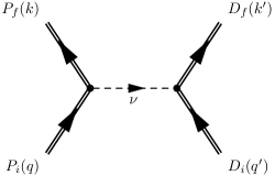
It is well known by now that neutrino oscillations can be consistently described either in the quantum-mechanical (QM) wave packet approach, or within a quantum field theoretic (QFT) framework.111Although in a number of sources a plane wave approach to neutrino oscillations is employed, it is actually marred by inconsistencies and, if applied correctly, does not lead to neutrino oscillations at all Rich:1993wu , Beuthe1 . In the QM method Nussinov:1976uw , Kayser:1981ye , Giunti:1991ca , Rich:1993wu , Kiers , Dolgov:1997xr , Giunti:1997wq , Cardall:1999ze , Dolgov:1999sp , Dolgov:2002wy , Giunti:2002xg , FarSm , Visinelli:2008ds , AS , nuwp2 , neutrinos produced in weak-interaction processes are described by propagating wave packets, the spatial length of which is related to the momentum uncertainty at neutrino production, and the detected states are also described by wave packets, centered at the detection point. The transition (oscillation) amplitude is then obtained by projecting the evolved emitted neutrino state onto the detection state. In the QFT treatment Kobzarev:1980nk , Kobzarev:1981ra , Giunti:1993se , Rich:1993wu , Grimus:1996av , Grimus:1998uh , Ioannisian:1998ch , Cardall:1999ze , Dolgov:1999sp , Beuthe2 , Dolgov:2002wy , Dolgov:2004ut , Dolgov:2005nb , AKL1 , one considers neutrino production, propagation and detection as a single process, described by a tree-level Feynman diagram with the neutrino in the intermediate state (see fig. 1). Neutrinos are represented in this framework by propagators rather than by wave functions. Both approaches lead to the standard formula for the probability of neutrino oscillations in vacuum in the case when the decoherence effects related to propagation of neutrinos as well as to their production and detection can be neglected. They differ, however, in the way they account for possible decoherence effects, with the QFT approach leading to a more consistent and accurate description. The QM method treats neutrino energy and momentum uncertainties responsible for these effects in a simplified way; in addition, it involves an ad hoc normalization procedure for the transition amplitude that is not properly justified.
The goal of the present paper is to compare the two approaches and establish a relationship between them, as well as to clarify some of the procedures that are employed in the QM method from the more general and consistent QFT standpoint. Some work in that direction has been done before. In Giunti:2002xg neutrino wave packets were derived starting from the QFT formalism (see also a discussion in Beuthe1 ). In Kopp:2009fa , a comparison of the QM and QFT approaches was presented for the special case of Mössbauer neutrinos, i.e. neutrinos produced and detected recoillessly in hypothetical Mössbauer-type experiments (see, e.g., Raghavan:2005gn , AKL1 , Potzel:2008xk and references therein). The new results obtained in the present work include a more advanced and general study of the QFT-based derivation of the neutrino wave packets (including the possibility that some of the external particles are not detected), matching of the QFT and QM expressions for the neutrino wave packets, study of the general properties of the wave packets describing the neutrino states (including their energy uncertainties in the case when neutrinos are produced in decays of unstable particles) and clarification of the issue of normalization of the oscillation probabilities in QM and QFT.
The paper is organized as follows. To make the presentation self-contained, in Secs. 2 and 3 we review, respectively, the QM wave packet formalism and the QFT approach to neutrino oscillations. Sections 4 – 6 contain our main results. In Sec. 4 we discuss how the neutrino wave packets, which are a necessary ingredient of the QM approach, can be derived starting from the QFT formalism. Next, we consider some general properties of the neutrino wave packets and discuss the conditions under which they can be approximated by Gaussian wave packets. Using the case of Gaussian wave packets as an example, we then discuss how the QFT-derived wave packets can be represented in the form usually adopted in the QM treatment. We also find expressions for the effective parameters describing the QM wave packets in terms of the more fundamental input parameters of the QFT framework. Next, we discuss the neutrino energy uncertainty in the case when neutrinos are produced in decays of unstable particles. In Sec. 5 we consider the problem of normalization of the neutrino wave packets in the QM framework and show how the normalization problem is solved in a natural way in the QFT-based approach. In Sec. 6 we discuss how one can relax some assumptions usually adopted in the QM and QFT approaches. Those include the assumption that the maxima of wave packets of all particles involved in the neutrino production (or detection) process meet at one space-time point, as well as the assumption that the mean momenta of the emitted and detected neutrino wave packets coincide. We summarize our results and conclude in Sec. 7. Some technical material is included in Appendices A and B.
2 Review of the QM wave packet formalism
We start with some generalities that are common to QFT and QM and then move on to review the QM wave packet approach to neutrino oscillations. We shall use the natural units throughout the paper.
In quantum theory, one-particle states of particles of type can be written as
| (1) |
where is the one-particle momentum eigenstate corresponding to momentum and energy (for free particles, , being the mass of the particle), is the momentum distribution function with the mean momentum , and we use the shorthand notation
| (2) |
For particles with spin, the states and depend also on a spin variable, which we suppress to simplify the notation. We will also often omit the second argument of where this cannot cause confusion.
We choose the Lorentz invariant normalization condition for the plane wave states :
| (3) |
The standard normalization of the states then implies
| (4) |
The quantity is actually the momentum-space wave function of : . The time dependent wave function is , where and is the free Hamiltonian of . The coordinate-space wave function is the Lorentz-invariant Fourier transform of :222 Recall that the Fourier transformation is based on the completeness condition for 1-particle momentum eigenstates, which for our normalization convention reads (see, e.g., PeskSchr , eq. (2.39)). Here the right hand side is the unit operator in the subspace of 1-particle states and zero in the rest of the Hilbert space. Note that the integration measure is Lorentz invariant.
| (5) |
or
| (6) |
In the QFT framework, it can be written as
| (7) |
where and is the second-quantized field operator of . Using the standard decomposition of the field in terms of production and annihilation operators, one can readily obtain (5) from (7) and (1). Note that expressions (5) and (6) can describe both bound states and propagating wave packets (in the case of bound states or particles propagating in a potential, the relation simply has to be replaced by the proper dispersion relation). A wave packet is obtained when the momentum distribution function is sharply peaked at or close to a nonzero mean momentum ,333The peak momentum coincides with the mean momentum for symmetric wave packets. i.e. when the momentum dispersion satisfies ; for the rest of this section we will assume this to be the case. The wave function (6) then describes a wave packet whose maximum of amplitude is located at at time . A wave packet that is peaked at coordinate at time is obtained by acting on the state by the space-time translation operator , where is the 4-momentum operator. For the coordinate-space wave function this yields
| (8) |
instead of eq. (6).
Eqs. (6) and (8) represent wave packets that propagate with the group velocity and in general spread with time both in the longitudinal direction and in the directions transverse to their mean momentum. The spreading is due to the fact that different momentum components of the wave packet have slightly different velocities .
Let us now consider neutrino oscillations in the framework of the QM wave packet formalism, sometimes also called the “intermediate wave packet” approach. Neutrinos produced or absorbed in charged-current weak interaction processes are considered to be flavour eigenstates (, which are coherent linear superpositions of mass eigenstates ( with coefficients given by the elements of the leptonic mixing matrix . The mass eigenstates are represented by the corresponding wave packets. If a neutrino of flavour was produced at time at a source centered at , its momentum-space wave function at a time is
| (9) |
Here the subscript shows that the wave packet corresponds to a neutrino produced at the source. Note that the index at simply indicates that the emitted neutrino was of flavour at its production time ; it is, of course, no longer so for . The shape of the wave packet of the th mass-eigenstate neutrino is given by the momentum distribution function , which is determined by the mechanism and conditions of neutrino production. In the QM framework, however, the neutrino production and detection processes are not explicitly taken into account; therefore the functions are postulated rather than determined, with the corresponding momentum widths estimated from the localization properties of the production process. Usually, the wave packets are taken to be of the Gaussian form
| (10) |
where characterizes the momentum uncertainty of the produced neutrino state, and similarly for the state of the detected neutrino. The advantage of Gaussian wave packets is that they allow most calculations to be done analytically (the same is also true for Lorentzian wave packets, see ref. Kopp:2009fa ).
The state of the detected neutrino is described by a wave packet peaked at the detection coordinate . In the momentum-space representation it is given by
| (11) |
where the subscript stands for detection. The momentum distribution functions are governed by the properties of the detection process; however, just as for neutrino production, in the QM approach these functions are postulated rather than determined. Note that, although the assumption is adopted in most studies, in general there is no reason to expect the mean momenta of the produced and detected wave packets to coincide. We will discuss this point in more detail in Sec. 6.
The amplitude for the transition is obtained by projecting the evolved neutrino production state onto the detection state:
| (12) |
where is the detection time, and . Performing the projection in momentum space, we obtain from (9) and (11) 444Projection in momentum space will turn out to be convenient for our subsequent discussion. The coordinate-space projection yields, of course, the same result.
| (13) |
For future reference, we shall also write this as a superposition of the amplitudes corresponding to the contributions of different neutrino mass eigenstates:
| (14) |
with
| (15) |
The oscillation probability is given by the squared modulus of the transition amplitude: . Since in most experiments the neutrino emission and detection times are not measured, the standard procedure is then to integrate over . This gives
| (16) |
Substituting here the transition amplitude (13) yields, up to a normalization factor, the standard probability of neutrino oscillations in vacuum provided that all decoherence effects are negligible. The normalization factor can then be fixed by requiring that the oscillation probability satisfy the unitarity condition (see Sec. 5 for a more detailed discussion).
3 Neutrino oscillations in QFT
In the QFT approach (which is sometimes also called the “external wave packet” formalism), neutrino production, propagation, and detection are considered as a single process, described by the Feynman diagram shown in fig. 1, with the neutrino in the intermediate state. In our overview of the QFT formalism we will mostly follow ref. Beuthe1 . Assume that the neutrino production process involves one initial state and one final state particle (besides the neutrino). Likewise, we will assume that the detection process involves only one particle besides the neutrino in the initial state and one particle in the final state. The generalization to the case of an arbitrary number of particles involved in the neutrino production and detection processes is straightforward and would just complicate the formulas without providing further physical insight. All external particles will be assumed to be on their respective mass shells.555 Since only one particle is assumed to be in the initial state of the production process, it must be unstable. This will be of no importance for us here because, as was already mentioned, the results are easily generalized to the case of an arbitrary number of external particles. Possible instability of the parent particle will be taken into account in Sec. 4.4.
The states describing the particles accompanying neutrino production and detection (“external particles”) can be represented in the form (1). For the initial and final states at neutrino production we can write
| (17) |
and similarly for the states accompanying neutrino detection:
| (18) |
We assume these states to fulfill the normalization condition (4). Some (or all) of the mean momenta of the external particles , , and may vanish, i.e. the states in eqs. (17) and (18) can describe bound states at rest as well as wave packets.
The amplitude of the neutrino production - propagation - detection process is given by the matrix element
| (19) |
where is the time ordering operator and is the charged-current weak interaction Hamiltonian.666We consider neutrino production and detection at energies well below the -boson mass, so that is the effective 4-fermion Hamiltonian of weak interactions. Note that no neutrino flavour eigenstates have to be introduced in the QFT framework, and the indices and simply refer here to the flavour of the charged leptons participating in the production and detection processes.
From eq. (19) it is easy to calculate the transition amplitude in the lowest nontrivial (i.e. second) order in using the standard QFT methods. The resulting expression corresponds to the Feynman diagram of fig. 1 and can be written as
| (20) | |||||
Here the sum runs over all intermediate states (i.e. different neutrino mass eigenstates), and the quantity is the plane-wave amplitude of the process with the th neutrino mass eigenstate propagating between the source and the detector:
| (21) |
Here and are the 4-coordinates of the neutrino production and detection points, the quantities and are the plane-wave amplitudes of the processes and , respectively, with the neutrino spinors and excluded. The choice of the 4-coordinate dependent phase factors corresponds to the assumption that the peaks of the wave packets of particles involved in the production process are all located at at the time , whereas for the detection process the corresponding peaks are all situated at at the time (we will discuss in Sec. 6 how this assumption can be relaxed). The integral in the second line of eq. (21) gives the coordinate-space propagator of the th neutrino mass eigenstate.
It is convenient to switch to shifted 4-coordinate variables , , defined according to , . Taking into account that , one can then rewrite eq. (21) as
| (22) |
where
| (23) |
are the full amplitudes (with the neutrino spinors included) of the processes and , respectively, and we have taken into account that the matrix elements and involve the left-handed chirality projection, so that only the left-handed spinors and contribute to the sum over the neutrino spin variable .
4 Comparing the QM and QFT approaches to neutrino oscillations
Let us now compare the results of the QM and QFT approaches to neutrino oscillations. Consider first the transition amplitude (24) obtained in the QFT formalism. The integration over the neutrino 4-momentum in this expression can be done in different order. Here it will be more convenient for us to integrate first over and then over (the opposite order will be used in Sec. 5). Since the distance between the neutrino source and detector is macroscopic, the phase factor in the integrand of eq. (24) undergoes fast oscillations and the integral is strongly suppressed except when the intermediate neutrino is on the mass shell. Thus, the dominant contribution to the integral is given by the residue at the pole of the neutrino propagator at ,777The contribution of the pole at is strongly suppressed due to an approximate conservation of mean energies at production and the fact that . where
| (26) |
Eq. (24) can therefore be rewritten as
| (27) |
where is the Heaviside step function.
4.1 Deriving neutrino wave packets in the QFT-based approach
Let us now compare eqs. (27) and (13). We see that the two equations are of the same form and actually coincide if we identify the QM wave packets as
| (28) |
where the functions and were defined in eq. (25).
The obtained result can be easily understood. Indeed, as follows from the definition of , for (i.e. on the mass shell of ) this quantity is the probability amplitude of the production process in which the th mass eigenstate neutrino is emitted with momentum ; but this is nothing but the momentum distribution function of the produced neutrino, i.e. the momentum-state wave packet . A similar argument applies to the neutrino detection process and . The wave packets and in eq. (28) are not normalized according to (4), though they can be easily modified to satisfy this condition. However, as we shall see in Sec. 5, this is not necessary and actually would be misleading.
An alternative method of deriving neutrino wave packets in the QFT framework, based on the S-matrix approach, was suggested in Giunti:2002xg ; the obtained results are equivalent to those in eqs. (28) and (25).
Let us now consider the wave packet describing the produced neutrino state in more detail (the state of the detected neutrino can be studied quite analogously). According to (28), the momentum distribution function characterizing the state of the emitted neutrino of mass is essentially given by the on-shell function . Since the matrix element is a smooth function of the on-shell 4-momenta and , whereas the wave packets of the external states are assumed to be sharply peaked at or near the corresponding mean momenta, one can replace by its value at the mean momenta and pull it out of the integral. Eqs. (25) and (28) then yield
| (29) |
where the 4-momenta and are defined as
| (30) |
From eq. (29) (or eqs. (25) and (28)) one can draw some important conclusions about the properties of the neutrino momentum distribution functions which determine the emitted neutrino wave packets:
-
•
Since the quantities and depend only on the properties of the external particles, and the -dependence of the matrix elements comes through the on-shell neutrino spinor factors , which depend on only through the neutrino energy, the functions depend on the index solely through the neutrino energy . This, in particular, means that for ultra-relativistic or quasi-degenerate in mass neutrinos the momentum distribution functions of all neutrino mass eigenstates are practically the same (provided that their energy differences are small compared to the energy uncertainty ).
-
•
Because the integral over the 3-coordinate in eq. (29) yields , and the momentum distribution functions and are sharply peaked at or near their respective mean momenta and , the neutrino momentum distribution functions are sharply peaked at or close to the momentum , with the width of the peak dominated by the largest between the momentum uncertainties of the states of and .
Taking into account eq. (5), eq. (29) can be rewritten as
| (31) |
Thus, the momentum distribution function that determines the wave packet of the emitted neutrino is essentially the 4-dimensional Fourier transform of the product of the coordinate-space wave functions of the external particles participating in the neutrino production process, taken under the condition that the components of the neutrino 4-momentum are on the mass shell. Eq. (31) can be readily generalized to the case when more than two external particles participate in the neutrino production process: the expression in the integrand of (31) should simply be replaced by the product of the wave functions of all particles in the initial state of the production process and of complex conjugates of the wave functions of all particles in the final state (except the neutrino).
The neutrino wave packet in coordinate space is obtained from eq. (31) by performing the Fourier transformation over the 3-momentum variable according to the transformation law (6), which gives
| (32) |
Here and we have used eq. (23) to extract the -dependent factor from . The integral over in eq. (32) can be expressed in terms of the modified Bessel function Gradshtein , giving
| (33) |
where . The integral in the second line of eq. (32) is greatly simplified in the limit of vanishing neutrino mass:
| (34) |
Note, however, that in this limit all neutrino species travel with the same speed and therefore the wave functions in eq. (34) cannot describe decoherence due to the separation of wave packets. In order to take possible wave packet separation effects into account the more accurate expression (33) has to be used. Alternatively, one can employ the momentum-representation wave function (31).
Expression (33) for the wave function of the produced neutrino state allows a simple interpretation. Note that is the scalar retarded propagator in the coordinate representation. Therefore the neutrino wave packet (33) is essentially the convolution of the neutrino source (the role of which is played by the neutrino production amplitude ) with the retarded neutrino propagator, in full agreement with the well known result of QFT. Note that only the scalar part of the propagator contributes to ; this is because the coordinate space and momentum space neutrino wave functions and are scalars in our formalism. The spinor factors are included in the matrix elements and (note that these quantities are also scalar, whereas the amputated matrix elements and , i.e. those with the neutrino spinors removed, have spinorial indices).
In our discussion of the wave packets of the emitted neutrino states, we were assuming that the momentum distribution functions of all the external particles accompanying neutrino production are known. This implies, in particular, that all particles in the final state of the production process are “measured”, either by direct detection or through their interaction with the medium in the process of neutrino production. It is quite possible, however, that some of the particles accompanying neutrino production escape undetected; this is, e.g., the case for atmospheric or accelerator neutrinos born in the process , in which the final state muon is normally not detected. It is also possible that some of the particles accompanying neutrino detection are “unmeasured”. How can one determine the neutrino wave packets in those cases?
To answer this question, let us recall that the momentum uncertainty characterizing the emitted neutrino depends in general on the momentum uncertainties of all the external particles at neutrino production and is dominated by the largest among them (see the discussion after eqs. (29) and (30)). In particular, in the case of Gaussian wave packets, one has Giunti:2002xg , Beuthe1
| (35) |
For more than two external particles at production, the sum on the right-hand side of this relation would contain the contributions of the squared momentum uncertainties of all these particles. Now, if a particle goes “unmeasured” in the neutrino production process, its momentum uncertainty cannot affect the momentum uncertainty of the emitted neutrino state and therefore can be neglected. To put it differently, undetected particles are completely delocalized, and therefore, according to Heisenberg’s uncertainty relation, have vanishing momentum uncertainty. This means that undetected particles can be represented by states of definite momenta, i.e. by plane waves. If, for example, the particle at production is undetected, one has to replace in eq. (29) the momentum distribution function by where is the normalization volume, and in eq. (31) the coordinate-space wave function by , with eqs. (32) - (34) modified accordingly. The mean momentum of the neutrino state depends, of course, on the momentum of the undetected particle; if the latter can take values in some range, the same will be true for the mean momentum of the emitted neutrino state. In this case the flux of emitted neutrinos will be characterized by a continuous spectrum.
In most of our discussion in this subsection we concentrated on the wave packets of the produced neutrino states. Our consideration, however, applies practically without changes to the detected neutrino states; the corresponding formulas can be obtained from eqs. (29) and (31)-(34) by replacing, where appropriate, , and .
4.2 General properties of neutrino wave packets
We have already considered some of the general properties of the neutrino wave packets in the previous subsection. In particular, we have found that the momentum distribution functions of mass-eigenstate neutrinos depend on the index only through the neutrino energy , and that the functions are sharply peaked at or near the momentum , with the width of the peak dominated by the largest between the widths of the functions and . Further insight into the general properties of the neutrino wave packets can be gained by comparing expressions (25) with their plane-wave limits. If the external particles were described by plane waves, the quantities and , which determine the neutrino wave packets, would be just equal to the matrix elements of the neutrino production or detection processes divided by the factor for each external particle and multiplied, correspondingly, by . The latter factors represent energy-momentum conservation at the production and detection vertices. As follows from (25), in the case when the external particles are described by wave packets, the quantities and (and therefore the momentum distribution functions of the neutrino wave packets) correspond to “smeared -functions”, representing approximate conservation of the mean energies and mean momenta of the participating particles. How exactly this smearing occurs will depend on the form of the wave packets of the external particles, and to move ahead one has to specify this form.
A particularly useful and illuminating example of a specific form of the external wave packets, and the one most often used in the literature, is the case of Gaussian wave packets. We will employ this example to illustrate the general properties of the neutrino wave packets.
Let us discuss first the conditions under which an arbitrary wave packet can be accurately approximated by a Gaussian one. For simplicity, we will consider here 1-dimensional wave packets. This is a good approximation in the case when the distance between the neutrino source and detector is very large compared to their sizes, so that the neutrino momentum is practically collinear with (the generalization to the 3-dimensional case is straightforward). Consider a wave packet described by a momentum distribution function , sharply peaked at some value of the momentum. We can write this function in the exponential form as
| (36) |
The Gaussian approximation corresponds to the case when the integral over of the function multiplied by any function of that is smooth in the vicinity of can be evaluated in the saddle point approximation. Indeed, in this approach one expands the function around its minimum at and keeps the terms up to and including the quadratic one:
| (37) |
This precisely means the wave packet is approximated by the Gaussian one. The validity condition for this approximation is given in terms of the derivatives of the function at :
| (38) |
It can be satisfied for a wide range of functions . However, it is easy to construct wave packets for which it is not satisfied. Consider, e.g. a class of wave packets
| (39) |
with integer and a constant, which can be found from the normalization condition for . It is easy to check that condition (38) is equivalent to . Thus, the momentum distribution functions (39) can be accurately approximated by the Gaussian ones only when . This condition, in particular, is not satisfied for Lorentzian wave packets.
4.3 Matching the QFT and QM neutrino wave packets
Let us now discuss how one can match the QFT and QM wave packets of neutrinos. Using the case of Gaussian wave packets as an example, we shall find out how the effective parameters describing the QM wave packets can be expressed in terms of the more fundamental parameters entering into the QFT approach.
We start by introducing some notation (we mostly follow Giunti:2002xg , Beuthe1 here). The coordinate uncertainty characterizing the wave function of the initial state particle in the neutrino production process is related to its momentum uncertainty by
| (40) |
and similarly for all other external particles. One can also introduce the effective coordinate uncertainty of the production process , which is connected to the effective momentum uncertainty of this process defined in eq. (35) by a relation similar to (40), or equivalently
| (41) |
This formula has a simple physical interpretation: since the neutrino production process requires an overlap of the wave functions of all the participating particles, the effective uncertainty of the coordinate of the production point is determined by the particle with the smallest coordinate uncertainty. This is in accord with the already discussed fact that the effective momentum uncertainty at production , which determines the momentum uncertainty of the produced neutrino, is dominated by the largest among the momentum uncertainties of all the external particles involved in neutrino production.
Next, we define the effective velocity of the neutrino source and its effective squared velocity as
| (42) |
If , they are approximately equal to, respectively, the velocity and squared velocity of the particle with the smallest coordinate uncertainty. We will also need the quantity defined through
| (43) |
This quantity can be interpreted as the effective energy uncertainty at neutrino production Beuthe1 . It can be also shown that , i.e. .
We can now discuss the results obtained in the QFT framework in the case when the external particles are represented by Gaussian wave packets. The function , which coincides with the momentum distribution function of the emitted mass-eigenstate neutrino , can be written as Giunti:2002xg , Beuthe1
| (44) |
where
| (45) |
is the normalization factor and
| (46) |
Here
| (47) |
and was defined in eq. (26). Note that in the limit when the external particles are represented by plane waves (, ), the first equation in (25) yields
| (48) |
as discussed in the previous subsection. From eq. (35) and the fact that it follows that in this limit the momentum uncertainty and energy uncertainty of the produced neutrino state vanish as well; thus, if the external particles are described by plane waves, then so is the produced neutrino. As follows from eq. (48), the plane wave limit corresponds to exact energy and momentum conservation at production.888Since the neutrino energy and momentum are completely determined by those of the external particles in this case, only one neutrino mass eigenstate can be produced in any given interaction process, and therefore no oscillations are possible in the plane wave limit Beuthe1 . This can also be seen from eqs. (44) and (46): indeed, in the limit the right hand side of (44) is proportional to the product of the energy and momentum conserving -functions. For finite values of and , eqs. (44) and (46) yield Gaussian-type “smeared delta functions”, i.e. describe approximate conservation laws for the mean momenta and mean energies of the wave packets, for which are responsible, respectively, the first term and the second term in (46).
Let us now try to cast expressions (44) and (46) into the form usually adopted in the QM wave packet approach to neutrino oscillations. We want to reduce to an expression similar to that in eq. (10). To this end, we expand the neutrino energy around the point and keep terms up to the second order:
| (49) |
Here
| (50) |
The lower index corresponds to the neutrino mass eigenstates, while the upper indices and number the components of the 3-vectors , and (i.e. is the th component of the group velocity of the th neutrino mass eigenstate). The function defined in (46) can then be written as
| (51) |
where
| (52) |
| (53) |
Let us now try to represent in the form
| (54) |
with
| (55) |
where the parameters and are to be determined by comparing eqs. (54) and (51). They describe, respectively, a shift of the neutrino mean momentum compared to the naive expectation and a modification of the overall normalization of the neutrino wave function. The effective momentum uncertainty characterizing the QM neutrino wave packet can be obtained by diagonalizing the matrix . The squared uncertainties of the different components of the neutrino momentum are given, up to the factor 1/4, by the reciprocals of the eigenvalues of the matrix . In general, these eigenvalues are different, i.e. the neutrino momentum uncertainty is anisotropic. This actually means that expression (10) for a 3-dimensional Gaussian wave packet is oversimplified: its exponent has to be replaced by .
Comparing eqs. (54) and (51), one finds that the shift of the neutrino mean momentum satisfies the equation
| (56) |
whereas the parameter is given by
| (57) |
The full solutions of eqs. (56) and (57) are given in Appendix A; here we present the results obtained in the leading order in the small parameter .999That this parameter is indeed small can be readily seen from eqs. (44) and (46): the function is strongly suppressed unless . The diagonalization of the matrix gives in this limit
| (58) |
where the axis was chosen in the direction of . For and one finds
| (59) |
From eq. (58) it follows that the neutrino momentum uncertainty in the direction of is smaller than those in the orthogonal directions. Note that for non-relativistic sources () the direction of essentially coincides with that of the mean neutrino momentum, and eq. (58) means that the longitudinal uncertainty of the neutrino momentum is smaller than the transversal ones. To understand this property qualitatively, one can imagine the neutrino production region (i.e. the region where the wave packets of the particles involved in the production process have significant overlap) to be approximately spherical with radius of order . Then, the transverse extent of the neutrino wave packet will also be . On the other hand, its longitudinal spread is determined by the duration of the production process (i.e. the time interval during which the wave packets have significant overlap), which is given by , where is the relative velocity of the two external particles.
Summarizing the results of the current subsection, we can see that the QM neutrino wave packets can match those obtained in the QFT framework if one applies the following changes to the QM results:
-
•
The momentum uncertainties of the neutrino mass eigenstates are replaced by the effective ones, defined in eq. (58). They are in general different in different directions.
-
•
The mean momentum is shifted according to , where the components of are given in eq. (59).
-
•
The wave packet of each neutrino mass eigenstate gets an extra factor , where is given in (59).
From the last point one can see that if the differences of the energies of different neutrino mass eigenstates are small compared to the energy uncertainty ,
| (60) |
the additional factors are essentially the same for the wave functions of all neutrino mass eigenstates and can be included in their common normalization factor. If, on the contrary, this condition is violated, the coherence of the emission of different neutrino mass eigenstates will be lost AS .
As follows from eq. (58), the effective momentum uncertainties that should be used to describe the wave packets of emitted neutrinos in the QM formalism are not just equal to the true momentum uncertainty at production , as naively expected, but also depend on the energy uncertainty , which is an independent parameter, as well as on the neutrino velocity and the effective velocity of the neutrino production region . Except for , the momentum uncertainty along the direction of is dominated by the smaller between and , which turns out to be . This is related to the fact that neutrinos propagate over macroscopic distances and therefore are on their mass shell, which enforces the relation (see Sec. 5.2 of ref. AS ). In the limit , which corresponds to a stationary neutrino source approximation Beuthe1 , the effective longitudinal momentum uncertainty vanishes, even though the true momentum uncertainty is nonzero. This implies an infinite coherence length, in accordance with the well known result for the stationary case Kiers , Grimus:1996av . It also confirms the expectation that wave packets of Mössbauer neutrinos, which are emitted in a quasi-stationary process, have a very large spatial extent AKL1 , Akhmedov:2008zz .
We have discussed here the matching of the QFT and QM wave packets of the produced neutrino states; for the wave packets of the detected states the consideration is completely analogous.
4.4 The case of an unstable neutrino source
Let us now consider the situation when neutrinos are produced in decays of unstable particles. Once again, we will assume that the external particles are described by Gaussian wave packets. Compared to the standard formalism that leads to eqs. (44) and (46), one now has to introduce the following modifications:
-
1.
The energy of the parent particle acquires an imaginary part, i.e. one has to replace , where , being the rest-frame decay width of . This amounts to replacing the energy difference defined in (47) according to .
-
2.
The integration over time in the formula for in eq. (25) now has to be performed from 0 to rather than from to (assuming that is the production time of the parent particle ).
As a result of these modifications, eqs. (44), (46) get replaced by
| (61) |
where
| (62) |
with
| (63) |
and being the time of maximum wave packet overlap in the production region (see Sec. 3). The -dependent Gaussian factor in eq. (61) describes, as before, an approximate conservation of mean momenta at neutrino production, whereas the factor is responsible for an approximate conservation of mean energies. Unlike in the case of stable particles considered in Sec. 4.3, the latter does not have a Gaussian form. Note the different time dependence of the different terms in the exponent in the integrand of the first integral in (62): the terms proportional to and are multiplied by , whereas the term is multiplied by . This is because the former two terms reflect the fact that the peak of the wave packet of is located at the neutrino production point at the time , whereas the wave function of this particle exhibits an overall exponential suppression starting from its creation time .
Calculating the integral in (62), we find
| (64) |
where erf is the error function. The limiting cases of interest can now be obtained from the relevant expansions of this function, but it is actually easier to study them starting directly with the expression for in eq. (62).
Indeed, the integrand of contains the exponential and oscillating factors, and therefore the integration domain that gives significant contribution to is
| (65) |
provided that the right hand side of this condition does not exceed ; if it does, for negative the domain is limited by . Let us note that, while the parameter may vanish, cannot, as it has a non-zero imaginary part . Consider first the limit , , which implies
| (66) |
In this case one can set and also extend the lower integration limit in eq. (62) to , which gives . Substituting this into eq. (61) yields, up to the extra factor , the old result of eqs. (44) and (46). If instead of the second condition in (66) one considers the opposite limit , the lower integration limit in the last integral in (62) can be set equal to zero. Since the error function goes to zero for small arguments, if follows that the result in this case is just 1/2 of that in the case . Thus, we conclude that in the limit the approximate conservation of mean energies is given by the same (in this case Gaussian) law as in the case of the stable neutrino source, with the same energy uncertainty . This is an expected result.
Consider now the limit , , or 101010Note that the second condition in (67) cannot be relaxed: indeed, if one had , then would imply , and the wave function of the parent particle would be exponentially suppressed by the time the neutrino is produced.
| (67) |
In this case one can neglect the term in the exponent in the last integral in (62), which yields
| (68) |
This is the usual Lorentzian energy distribution factor corresponding to the decay of an unstable parent state.
Thus, we conclude that in the case when the factor in that is responsible for the approximate conservation of mean energies in the production process is essentially the same as in the case of a stable neutrino source (Gaussian in the case we considered), whereas in the opposite limit, , it is given by the Lorentzian energy distribution corresponding to the natural linewidth of the source . In the intermediate case , the energy-dependent factor in is neither Gaussian nor Lorentzian, with the effective energy uncertainty being of the same order as and .
5 Oscillation probabilities and the normalization conditions
5.1 Normalization of oscillation probabilities in the QM approach
In the QM wave packet approach to neutrino oscillations, one has to normalize the oscillation probability by hand by requiring that it satisfy the unitarity constraint
| (69) |
This is an ad hoc procedure that is not properly justified within the QM formalism; however, it seems to be unavoidable in that approach. In particular, one can readily make sure that the standard normalization of the neutrino wave packets , or, equivalently, , does not lead to the correct normalization of the oscillation probability (that this is indeed the case can be easily verified by using Gaussian wave packets as an example). Moreover, as we will show below, no independent normalization of the produced and detected neutrino states can lead to the correct normalization of the oscillation probability in the QM wave packet approach.
Let us now consider the unitarity constraints on the oscillation probabilities and their connection to the normalization conditions in more detail. As it is presented in eq. (69), the unitarity condition simply reflects the fact that during the propagation between the source and detector neutrinos are neither destroyed nor (re)created: once a neutrino is produced, it can only change its flavour.111111We neglect tiny probabilities of neutrino decay and absorption. Therefore, for a fixed initial flavour , the probabilities of neutrino conversion to all final flavours sum to unity. Note that the quantities by construction depend only on the distance between the source and the detector and not on the propagation time , which is integrated over (see eq. (16)).121212For simplicity we assume here the neutrino emission to be spherically symmetric. Otherwise, has to be defined as . Thus, the meaning of the unitarity condition (69) is that, once a neutrino is produced, the probability that it will be found at a given distance from the source at some time between zero and infinity is equal to one, provided that all flavour states are accounted for. Similarly, if one introduces , it will also satisfy a unitarity condition analogous to (69). In other words, once the neutrino is created, the probability to find it (in any flavour state) at a fixed time after its production somewhere in space is equal to one.
The unitarity conditions can only be satisfied if the oscillation probabilities are properly normalized. It is important to note, however, that in a consistent formalism unitarity must be satisfied automatically rather than being imposed by hand.
How about the un-integrated probability , should it satisfy a unitarity constraint similar to (69)? Obviously, for arbitrary and the answer to this question is negative. Indeed, unless where is the average group velocity of the neutrino wave packet and is its spatial length, the probabilities are vanishingly small for all and . Thus, unitarity cannot be used to normalize the un-integrated probability. The normalization of can, however, be fixed differently: in the limit , , i.e. when the produced neutrino did not have time to evolve yet, the probability must satisfy the initial condition . Note that the above limit should be understood in the sense that and are small compared to the oscillation length but large compared to, respectively, the sizes of the spatial localization regions and time scales of the neutrino emission and absorption processes. From eqs. (14) and (15) it then immediately follows that the amplitudes corresponding to neutrino mass eigenstates must satisfy where the real phase is the same for all . By a rephasing of the momentum distribution functions of either emitted or detected neutrinos, this common phase can be eliminated, and one finally gets .
Now, let us check if this condition is fulfilled in the particular case of Gaussian wave packets. For the momentum distribution functions of the produced and detected neutrino states normalized according to eq. (4), i.e. having the form (10), a straightforward calculation yields
| (70) |
For and both factors on the right hand side of the last equality are smaller than one, and therefore the condition is clearly violated. Moreover, the dependence of the result on the parameters of the produced and detected neutrino states does not factorize; this means that no independent normalization of these states can lead to the correct normalization of the amplitude, as pointed out above.
It is actually quite easy to understand why this happens. The integral in eq. (70) is nothing but the overlap integral of the wave functions of the produced and detected neutrinos. If these wave functions are normalized to unity and the momentum (or energy) spectra of the emitted and detected states do not coincide, this overlap integral is always less than one. In reality, the spectra of the emitted and absorbed neutrino states are determined by the physical nature and experimental conditions of the neutrino production and detection processes, which are always different. This, in particular, means that a fraction of the produced neutrinos may simply not be detectable. For instance, if the threshold in the detection process (either the physical threshold or the one imposed by energy cuts of the detected events) is higher than the maximum energy of the emitted neutrino, no detection will be possible at all. Mathematically, the fact that the overlap integral (70) is always less than one is a consequence of the Schwarz inequality , where the equality is only reached if .
Even if one adopts the unrealistic assumption (which for Gaussian wave packets would mean and ), this will not solve all the normalization problems of the QM wave packet approach. The condition will be satisfied in this case; however, the physically observable oscillation probability defined in eq. (16) will still not be properly normalized, and the unitarity condition (69) will not be satisfied. Indeed, from eq. (14) it follows that unitarity requires that AS
| (71) |
for all . Obviously, the fulfilment of the condition does not enforce (71); therefore in the QM formalism condition (71) has to be imposed by hand.
It is not difficult to understand why yet another normalization problem arises: integration over the time should actually be considered as time averaging in the QM approach, and the integral on the right hand side of eq. (16) should be normalized by dividing it by the characteristic time which depends on time scales of both the neutrino production and detection processes. This follows from the fact that the amplitude is substantially different from zero only when , where the effective length of the wave packet is determined by both the neutrino production and detection processes, which gives . It is difficult to calculate the quantity precisely, and the simplest way out is just to impose the unitarity condition by hand, which yields the correct normalization of .131313Note that once the normalization condition (71) is enforced, one can demonstrate that the resulting oscillation probability is Lorentz invariant AS . This is not trivial in the QM approach because the QM formalism is not manifestly Lorentz covariant.
Thus, in the QM approach there are two sources of the normalization problems: lack of the overlap of the wave functions of the produced and detected neutrino states and the necessity of integration over the neutrino propagation time . We will show now how both these problems are naturally solved in the QFT-based formalism.
5.2 Normalized oscillation probabilities in the QFT framework
5.2.1 Generalities
Let us start with recalling the operational definition of the neutrino oscillation probability. In a detection process that is sensitive to neutrinos of flavour , the detection rate is 141414We omit the obvious factors of detection efficiency and energy resolution that are not relevant to our argument.
| (72) |
where is the detection cross section and is the energy density (spectrum) of the flux at the detector. If a source at a distance from the detector emits neutrinos of flavour with the energy spectrum , the energy density of the flux at the detector is
| (73) |
where is the oscillation probability for neutrinos of energy , and we once again assumed for simplicity neutrino emission to be spherically symmetric. Substituting this into eq. (72) yields the rate of the overall neutrino production-propagation-detection process:
| (74) |
The oscillation probability can now be extracted from the integrand of eq. (74) by dividing it by the neutrino emission spectrum, detection cross section and the geometrical factor :
| (75) |
Note that an important ingredient of this argument is the assumption that at a fixed neutrino energy the overall rate of the process factorizes into the production rate, propagation (oscillation) probability and detection cross section. Should such a factorization turn out to be impossible, the very notion of the oscillation probability would lose its sense, and one would have to deal instead with the overall rate of neutrino production, propagation and detection.
Now let us come back to the QFT-based treatment of neutrino oscillations and try to cast the rate of the overall process in the form of eq. (74). To this end, we return to eq. (24) for the amplitude of the process but, unlike in the previous sections, perform in it the integration over 3-momentum before integrating over the energy variable . In doing so, we will make use of a result obtained by Grimus and Stockinger Grimus:1996av , which states that, for a large baseline , positive and a sufficiently smooth function ,
| (76) |
whereas for the integral behaves as . This result was obtained in Grimus:1996av in the limit , but a careful examination of the derivation shows that its applicability condition is actually , which we will assume to be satisfied. Applying (76) to eq. (24) yields
| (77) |
where
| (78) |
Next, we note that, just as the quantities depend on the index only through the neutrino energy , the functions depend on the index only through the neutrino momentum . Therefore, to simplify the notation we will denote
| (79) |
The overall probability of the neutrino production-propagation-detection process is the squared modulus of the amplitude (77):
| (80) |
We will actually need the integral of this probability over the time (the reasons for integration over will be discussed in Secs. 5.2.2 and 7):
| (81) |
We use the tilde here to stress that is not a probability but rather a time-integrated probability, which has the dimension of time. Note that (81) contains an incoherent sum (integral) over contributions from different energy eigenstates. This means that only the amplitudes corresponding to the same neutrino energy interfere, as it is in the stationary case. This is related to the integration over time and is a reflection of the fact that the time-integrated nonstationary probability is equivalent to the energy-integrated stationary probability Beuthe1 , AS . It should also be stressed that, although the integration over in eq. (81) is formally performed over the interval (recall that coincides with the variable of eq. (24)), the contribution of the unphysical region of negative energies is actually negligible and can be discarded. This is a consequences of the fact that are sharply peaked at positive values of energy , with the peak widths satisfying .
To simplify the following consideration, we will once again assume that the neutrino production and detection processes are isotropic. In our approach this means that we have to average the quantities and over the directions of the incoming particles and , which amounts to averaging over the directions of . We can therefore denote and drop from the arguments of in eq. (81) and all the subsequent expressions. Relaxing the isotropy assumption would complicate the analysis but would not change the final result for the probability of neutrino oscillations.
The next step is to calculate the neutrino production and detection probabilities. As can be seen from eq. (24), neutrinos in the intermediate state are considered in our framework as plane waves weighted with the factors . We therefore describe the external particles by wave packets and neutrinos by plane waves. Application of the standard rules of QFT then yields 151515Note that we do not include the factor in the integration measure because it is already included in the definition of , see eqs. (23) and (25).
| (82) |
The spectral density of emitted neutrino flux, , is obtained by removing the integration over energy on the right hand side of the last equality in (82).
For the detection probability we obtain
| (83) |
where the normalization volume comes from the plane-wave description of the incoming neutrino. Note that the expression for the production probability in eq. (82) does not contain the factor even though it is also calculated for plane-wave neutrinos. This is because neutrinos are in the final state at production, and the calculation of their phase space volume involves integration over .
5.2.2 The case of continuous fluxes of incoming particles
A direct inspection of the expressions for the probabilities of neutrino production and detection as well as of the probability of the overall production-propagation-detection process obtained above shows that they are independent of the total running time of the experiment . This is because they were calculated for individual processes with single external wave packets of each type, and the microscopic production and detection time intervals were assumed to be centered at fixed instants of time and , respectively. On the other hand, in practice one is usually interested in the total probabilities for the processes to occur within a macroscopic time interval of length or in interaction rates. Normally, the probabilities are proportional to , while the rates are -independent. In the wave packet approach, this can be achieved if we take into account that in realistic situations one often has to deal with continuous fluxes of incoming particles. (We will comment on the opposite case of stationary initial states in the next subsection.)
Let us start with calculating the production rate and detection cross section in the case of steady fluxes of the incoming particles. Consider some interval of time that is large compared to the time scales of the neutrino production and detection processes. Let the number of the projectile particles entering the production region (e.g. a spherical region of radius around the point ) during this interval be . Then the number of particles entering the production region during the interval is .
If the production probability in the case of the individual process with single external wave packets is , the probability of neutrino emission during the finite interval of time () is 161616 If the flux of the incoming particles is not steady, the number of particles entering the production region over the time is given by , where is the distribution of these particles with respect to , normalized according to . The right hand side of the first equality in eq. (84) then has to be replaced by . For a steady flux the distribution is uniform, i.e. .
| (84) |
The integration is trivial because is actually independent of due to invariance with respect to time translations. Note that the probability is proportional to . We can therefore define the production rate in the usual way:
| (85) |
Let us now consider the detection cross section. Normally, a cross section is defined for a single, fixed target particle. However, the initial-state particles in our treatment of the detection process are described by moving wave packets, which enter the detection region that is centered at a fixed point . Therefore, our treatment of neutrino detection should be similar to that of the production process. For the individual detection process with single external wave packets of each type the detection probability is given by eq. (83). Let us now assume that the number of the particles entering the detection region during the interval of time is . Then we obtain for the time-dependent detection probability in the case of steady incoming fluxes of and neutrinos
| (86) |
and for the detection rate
| (87) |
To obtain the detection cross section we have to divide this rate (more precisely, the summand of the sum over that enters into (87)) by the flux of incoming neutrinos , where is the number density of the detected and is their velocity. With our normalization (one particle in the normalization volume) we have , and from eqs. (83) and (87) we finally obtain
| (88) |
Now we proceed to the calculation of the rate of the overall production-propagation-detection process. Since we want to calculate this quantity not for a single process with individual wave packets of external particles but for steady fluxes of incoming and , we have to integrate the -dependent probability of the single process given by eq. (80) over both and . Proceeding in the same way as before, we find for the probability of the process for steady fluxes of the incoming particles
| (89) |
Introducing the new integration variables and , we obtain
| (90) |
It can be readily shown that in the limit of large (much larger than the time scales of the neutrino production and detection processes) the integral coincides with the quantity defined in eq. (81), whereas and give negligible contributions (see Appendix B). Therefore for large eq. (90) can be rewritten as
| (91) |
The rate of the overall process is then 171717 For the reader willing to check the dimensions of our expressions, we note that from the definitions of it follows that they have dimension . It is then easy to see that the amplitude (77) and the probabilities (81)-(84), (86), (89) and (91) are dimensionless, the cross section (88) has the dimension of squared length (or ), and the rates (85), (87) and (92) have the dimension of inverse time (or ), as they should.
| (92) |
5.2.3 The case of stationary initial states
If the initial state particles and/or are in stationary states rather than being described by moving wave packets, the above consideration has to be slightly modified. Consider, for example, neutrino production in decays of unstable particles bound in a solid. Let be the probability distribution function for the decay times of the parent particles in the source, and let be defined by the condition . If is short compared to the lifetime of , one has . If, on the contrary, , will usually have an exponential form.181818An exception is the case where in the source are continuously replenished. In this case, the function will depend on the time dynamics of the production of these particles. The neutrino production probability is then again given by eq. (84), just as in the case of a continuous flux of incoming particles .
The situation with bound-state stationary particles in the detector can be considered quite similarly. One can assume to be stable. If the source creates a steady flux of neutrinos, then for the ensemble of in the detector the distribution of the detection times is uniform and is given by , where is defined by the normalization condition . The detection probability is then given by eq. (86).
Thus, with these re-interpretations of and , the expressions for the neutrino production and detection probabilities and rates and the detection cross section obtained in the previous subsection remain valid in the case of stationary initial states as well.
We are now in a position to obtain the normalized oscillation probability.
5.2.4 The oscillation probability in the QFT approach
In the case when the rate of the overall production-propagation-detection process at a fixed neutrino energy factorizes, the oscillation probability should be obtainable from eq. (75). Substituting eqs. (92) and (85) (with and defined in eqs. (81) and (82)) and eq. (88) into this relation, we find
| (93) |
The quotation marks here are to remind us that we yet have to prove that this quantity can indeed be interpreted as the oscillation probability.
The alert reader has probably noticed that, while the integral in (74) is taken over the energies of different neutrinos in the neutrino flux, the integration in (81) is performed over the energy distribution within the wave packet of an individual neutrino. This, however, does not invalidate our argument leading to eq. (93). The reason for this is that the following two situations are known to be experimentally indistinguishable Rich:1993wu , Kiers : (a) a flux of neutrinos described by identical wave packets, each with an energy spread , and (b) a flux of neutrinos, each with a sharp energy, with the overall energy distribution .
Let us now discuss the conditions under which eq. (93) is a well-defined oscillation probability. For this to take the place, the expression for the differential rate of the overall process should factorize into the production rate, the oscillation probability, and the detection cross section. This means that it should be possible to pull the differential flux and the detection cross section out of the numerator of eq. (93) in analogy to eq. (74), and then cancel them against the denominator. This, in turn, requires that the momentum distributions and be virtually independent of the neutrino mass eigenstate index . To see when this is the case, we first note that the momentum distribution functions are all peaked at the same momentum . Therefore, if is much smaller than the width of the peak , we can replace the factors in eq. (93) by the common value calculated at the average momentum , pull them out of the sums in the numerator and in the denominator, and cancel them.191919It should be stressed that the mean momentum is defined here as an average over different mass eigenstates of the momenta taken at the same fixed value of energy . It is therefore different from the mean momentum of the individual wave packets, introduced earlier, for which the average was taken over the spread of momenta (or energies) within the wave packet. A similar argument applies to the momentum distribution functions associated with the detection process, , which are all peaked at the same momentum and have widths . When neutrinos are ultra-relativistic or quasi-degenerate in mass, i.e. when
| (94) |
we can also replace , by in the denominator of eq. (93).202020Note that condition (94) is usually weaker than the requirement . The phase space regions where it is stronger, i.e. where , are usually far from the peaks of the momentum distribution functions and are therefore suppressed. We can then use unitarity of the leptonic mixing matrix to reduce eq. (93) to
| (95) |
Since for ultra-relativistic or quasi-degenerate neutrinos , this is just the standard formula for the probability of neutrino oscillations in vacuum. Thus, the QFT-based approach allows one to identify the conditions under which can be sensibly defined, and also gives the correctly normalized expression for this probability. The conditions are that neutrinos should be ultra-relativistic or quasi-degenerate in mass and, in addition, the inequality
| (96) |
should be satisfied. Here, we have introduced the effective momentum uncertainty , which is dominated by the smallest between and . Since and , in turn, are dominated by the energy uncertainties and , repectively (see Sec. 4.3), condition (96) is equivalent to the one in eq. (60).
If condition (96) is violated, at least one of the momentum distributions , , , will be strongly suppressed. This implies that the numerator of eq. (93) will not factorize in accordance with eq. (74) in this case, so that the oscillation probability will not be a well-defined quantity. Also, eq. (93) will in general not satisfy the unitarity condition (69). It is important that the interference terms involving the suppressed momentum distributions in the numerator of eq. (93) will be quenched in this case, and thus neutrino oscillations involving the corresponding mass eigenstates will be inhibited. Physically, this can be traced to the lack of coherence at neutrino production and/or detection. It can be shown that production or detection decoherence is equivalent to the lack of localization of, respectively, the production or detection process Kayser:1981ye , Rich:1993wu , AS .212121While condition (96) ensures the production/detection coherence (localization), it says nothing about another possible source of decoherence – separation of neutrino wave packets at long enough distances due to the difference of the group velocities of different neutrino mass eigenstates. This is related to the fact that a fixed neutrino energy corresponds to the stationary situation, when the coherence length . The finite coherence length is recovered upon the integration over energy in eq. (81) Beuthe1 .
The above QFT-based considerations also allow one to shed some light on the meaning of the normalization condition imposed on the oscillation probability in the QM wave packet approach, which looks rather arbitrary within the QM framework. As was pointed out in Sec. 4.1, the QM and QFT approaches can be matched if the QM quantities and are identified with the QFT functions and , respectively. The latter, however, bear information not only on the properties of the emitted and absorbed neutrinos, but also on the production and detection processes. The QM normalization procedure that is tailored to obtain an expression for the oscillation probability satisfying the unitarity condition can then be easily seen to be equivalent, in the limit (96), to the division of the overall rate of the process by the production rate and detection cross section, as in eq. (93).
6 Some additional comments
In this section we will comment on some issues pertaining to the description of neutrino oscillations in the external and intermediate wave packet approaches that were not discussed or were only briefly mentioned above. We will also show how one can relax some assumptions usually adopted in the QM and QFT approaches.
1. Unequal mean momenta of the produced and detected neutrino states
In the vast majority of derivations of the neutrino oscillation probability within the QM wave packet framework, it was assumed that the mean momenta of the produced and detected neutrino states, and , coincide. 222222The only exceptions we are aware of are refs. AS , Kopp:2009fa . There are, however, no reasons for this to be the case. Indeed, the mean momenta of the emitted and absorbed neutrino states are determined by the kinematics and experimental conditions of the neutrino production and detection processes, respectively, and those are in general different. Let us now examine the consequences of using, as before, the case of Gaussian wave packets as an example.
It was shown in Sec. 4.3 that the neutrino wave packets derived in QFT can be cast into the form usually adopted for neutrino wave packets in the QM approach if one uses for the latter the effective (in general anisotropic) momentum uncertainties, shifted mean momenta and modified normalization factors. Since the expressions for the QM wave packets look simpler, we will study the implications of unequal mean momenta of the produced and detected neutrino states within the QM formalism. We will also ignore possible anisotropy of the neutrino momentum uncertainties. Taking it into account would just complicate the calculations without changing the essence of the result.
We will now calculate the amplitude (15) corresponding to the emission and absorption of the neutrino mass eigenstate . To do so, we expand the energy around a momentum which we do not specify for now:
| (97) |
An important point is that, strictly speaking, using such an expansion in the integral in (15) is only justified if and are not too far from each other and if , which we will assume. As we shall see, under these conditions the final result will be insensitive to the choice of the expansion point . In eq. (97) we have neglected higher order terms in the expansion; this corresponds to neglecting the spreading of the neutrino wave packets, which is unimportant for our argument.
The Gaussian wave packets for the produced neutrino states are given by eq. (10), and the detected wave packets have a similar form, with and replaced by and , respectively. Substituting these expressions and expansion (97) into eq. (15) yields, after a simple Gaussian integration,
| (98) |
Here
| (99) |
and we have used the relation which follows from (97). As can be seen from eq. (98), the dependence on the expansion point has completely disappeared from the amplitude.
The meaning of the obtained result is quite transparent: as usual, the amplitude contains a normalization factor, a plane wave factor calculated at some mean momentum (in this case ) and the envelope factor . However, on top of this, it contains the extra factor , which is a reflection of the approximate conservation of the mean neutrino momentum. It suppresses the amplitude unless the difference of the mean momenta of the produced and detected neutrino states is small compared to the effective total momentum width . Note that this width is dominated by the larger of and , unlike the momentum width defined in (99), which is dominated by the smaller of them.
2. Non-central collisions
In our discussion of the external wave packet formalism, as well as in all other treatments of this topic we are aware of, it was assumed that the peaks of the wave packets of all the external particles participating in neutrino production (or detection) meet at the same space-time point. In other words, it was assumed that at production these peaks are all located at the point at the same time , whereas at detection the peaks of the wave packets of the external particles are all located at at the same time . Is this always true and how crucial is this assumption?
While in some situations, such as neutrino production in decays of unstable particles, such an assumption may indeed be justified, this is not in general so when neutrinos are born in scattering processes, where the collisions of the wave packets in the initial state may be non-central. Let us consider non-central collisions assuming, as before, only two external particles at production and two at neutrino detection (the generalization to an arbitrary number of external particles is straightforward). One obvious consequence of this is that the neutrino production and detection are only possible if the minimum distances between the peaks of the participating wave packets do not exceed significantly the sizes of, correspondingly, the production and detection regions. Consider the production process. We shall now assume that the wave packets of the external particles and are given by expressions of the type (8), with the phase factors in the integrand being and , respectively. This means that the peak of the wave packet describing is located at at the time , and the peak of the wave packet of is located at at the time . We will consider the positions of these peaks at the same time, i.e. we will take . It is natural to choose to be the value of this common time corresponding to the minimum distance between the two peaks, i.e. , .232323This is easily generalized to the case of more than two external particles. For instance, for three particles with peaks at , and the time can be chosen to correspond to the minimum of . The coordinate can then be chosen to lie anywhere between and on the line connecting them; in particular, one can choose or . Neutrino detection can be considered quite similarly.
One can now repeat the calculations presented in Sec. 3, arriving at the transition amplitude that can again be written in the form (24). However, the expressions for and in eq. (25) have to be modified: their integrands should be multiplied, respectively, by and , where and are the positions of the peaks of the wave packets representing and at detection at the time when the distance between these two peaks reaches its minimum. This can be taken into account by redefining the momentum distribution functions of the wave packets according to
| (100) |
The newly defined momentum distribution functions share a crucial feature with the old ones: they decrease rapidly when the deviation of the corresponding momenta from their peak values exceed the relevant momentum uncertainties (i.e. the widths of the peaks) , , or . In addition, the new momentum distributions do not exhibit fast oscillations when the momentum variations are smaller than, or of the order of, the corresponding widths of the peaks. Indeed, consider neutrino production. Our choice of implies that and . On the other hand, as we mentioned above, the production is only possible when the distance between the peaks of the wave packets of the external particles is smaller than, or of the order of, the size of the production region, which is of the order of . A similar argument applies to neutrino detection. Therefore the variation of the exponents of the exponential factors in eq. (100) is and these factors do not undergo fast oscillations across the peaks of the momentum distributions.
From the above considerations it follows that the properties of the redefined momentum distributions are essentially the same as those of the old ones. All the results of the present paper therefore apply to the case of non-central collisions as well, if one substitutes the original momentum distribution functions by those redefined according to eq. (100).
7 Discussion and summary
In this paper we have compared the quantum mechanical approach to neutrino oscillations, where neutrinos are described by wave packets, with the quantum field theoretical method, where they are represented by propagators connecting the neutrino production and detection vertices in a Feynman diagram, whereas the external particles are described by wave packets in order to localize the process in space and time. We have shown how the neutrino wave packets underlying the QM approach can be derived in QFT by comparing the QM and QFT expressions for the transition amplitude. Equivalently, the wave packet representing the emitted neutrino can be obtained as the convolution of the neutrino source (the production amplitude) with the retarded neutrino propagator, in accord with the well known result of QFT. Quite analogously, the wave packet of the detected neutrino can be obtained as the convolution of the neutrino detection amplitude with the advanced neutrino propagator, with the result then taken at the time corresponding to neutrino detection.
We have studied the general properties of QFT-derived wave packets representing the produced neutrino states and demonstrated that the wave packets of mass eigenstates depend on the index only through the neutrino energy , and that in the momentum representation they are given by the production amplitude multiplied by “smeared delta functions” describing approximate conservation of mean energy and mean momentum at production. The widths of these “smeared delta functions” are determined by the largest among the corresponding widths of the external particles involved in the neutrino production process. Similar conclusions apply to the wave packets of the detected neutrino states.
We also identified the conditions under which general neutrino wave packets can be approximated by Gaussian ones. Using Gaussian wave packets as an example, we then demonstrated that the neutrino wave packets derived in QFT can be cast into the form they are usually assumed to have in the QM formalism, provided that
(i) The momentum uncertainty of the QM approach is replaced by the effective one, which depends not only on the true momentum uncertainty at production (or detection), but also on the corresponding energy uncertainty, as well as on the neutrino velocity and the effective velocity of the neutrino production (or detection) region. Moreover, these momentum uncertainties are different in different directions, i.e. are anisotropic. The longitudinal effective momentum uncertainties of the produced and detected neutrino states are dominated by the energy uncertainties characterizing, respectively, the neutrino production and detection processes, whereas the transverse effective momentum uncertainties coincide with the corresponding true momentum uncertainties.
(ii) The mean momentum of the neutrino state is shifted from its naively expected value.
(iii) The wave packets of different mass eigenstates acquire (in general different) extra overall factors.
Thus, the simplistic QM wave packet approach may need QFT-motivated modifications; however, once these modifications have been done, one can still work within the QM framework without losing any essential physical content.
We have also studied the energy uncertainties characterizing the neutrino wave packets in the case of unstable neutrino sources and have shown that in general these uncertainties depend both on the decay rate of the parent particle and on the inverse time scale of the overlap of the wave packets of the external particles. The neutrino energy uncertainty is dominated by the larger of the two.
In the last part of the paper, we have discussed in detail the normalization of the QM and QFT expressions for the oscillation probability . We have seen that in the QM framework has to be normalized by hand in order to fulfill the unitarity relation . There are two reasons why this ad hoc procedure is unavoidable in the QM approach. First, as we have demonstrated, no independent normalization of the produced and detected neutrino states can lead to the correct normalization of the oscillation probability because the overlap integral of these states is always smaller than unity in the realistic case when their momentum distributions are different. The overlap integral depends on the characteristics of the produced and detected states in a non-factorizable way, and so the problem cannot be cured by just modifying the normalization of these states. Second, the QM formalism involves an integration over the unobserved difference of the neutrino detection and production times , which leads to yet another undefined factor – the time interval by which one has to divide the result in order to recover the correct dimension of the oscillation probability. In the QM method both these problems are solved by imposing unitarity of the oscillation probability by hand.
We have demonstrated how the QFT approach avoids all the normalization problems of the QM formalism and we have derived the conditions under which it naturally leads to the correctly normalized oscillation probability that automatically satisfies the unitarity condition. The conditions are that (1) neutrinos are ultra-relativistic or quasi-degenerate in mass, and that, in addition, (2) the differences between the momenta of different neutrino mass eigenstates at fixed energy are much smaller than the widths of the neutrino momentum distributions determined by the production and detection processes. If these requirements are not fulfilled, the interaction rate cannot be factorized into the production rate, propagation (oscillation) probability and detection cross section, so that the oscillation probability is undefined. In that case one would have to deal instead with the overall rate of the neutrino production-propagation-detection process.
The QFT approach also allows one to understand the physical meaning of the QM normalization recipe: By imposing unitarity by hand one implicitly rids the calculated transition probability of the probabilities of neutrino production and detection, thus extracting the sought oscillation probability.
A comment on the the integration over is in order. Such an integration is involved in both the QM and QFT approaches to neutrino oscillations. In the QM framework, it has to be introduced to account for the fact that the neutrino’s time of flight is not measured (or at least not measured accurately enough) in realistic experiments. At the same time, in our QFT treatment of neutrino oscillations, it emerges naturally from the observation that in real situations one has to deal with continuous fluxes of incoming particles (or with ensembles of neutrino emitters and absorbers in the case of bound stationary initial states) rather than with individual acts of neutrino production, propagation and detection, in which single wave packets of the external particles of each type are involved. Can one still sensibly define an unintegrated oscillation probability for such a single act?
We will argue now that the probability is not a useful quantity since it is unmeasurable (or almost unmeasurable). An important point here is that in practice both and can only be measured with some accuracy. If we consider the -integrated probability which depends (in addition to neutrino energy) only on , then this quantity is well defined only if the error in the measurement of is small compared to the variations of over which the probability changes significantly. This means that this error must be small compared to the neutrino oscillation length , and this condition is normally easily satisfied. If one considers the case when the time is measured, whereas the distance is not (even though it is hard to imagine how such a situation could be realized in practice), then one would have to integrate over , and the resulting probability would be a function of . Then the situation would be similar – the error in the determination of would have to be small compared to the change of over which varies significantly, which is with the neutrino velocity.
The situation would be quite different if one considers the unintegrated probability which depends on both and – in this case the requirements on and would be by far more demanding. Indeed, is substantially different from zero only when , where is the spatial length of the neutrino wave packet. This means that for uncorrelated variations of and this probability varies significantly when changes by (which can be extremely small) and changes by . The latter quantity is essentially given by the largest between the time scales of the neutrino production and detection processes. Thus, the un-integrated probability can only be accurately measured if the distance is measured with an accuracy better than the length of the neutrino wave packet and simultaneously the time between neutrino emission and detection is measured with an error that is small compared to the duration of these processes. Such a possibility appears rather unrealistic at the very least.
It follows from our results that there are both intricate relations and important differences between the QM and QFT approaches to neutrino oscillations. In the following table, we compare the main features of these two approaches.
| QM approach | QFT approach | |
| 1. | Simple and transparent description of neutrino oscillations. Neutrino production and detection processes are not properly taken into account. Simplified description of neutrino energy and momentum uncertainties. | Most complete description of neutrino production, propagation and detection. Accurate treatment of neutrino energy and momentum uncertainties. The formalism is more complicated than that of the QM approach. |
| 2. | Produced and detected neutrino states are flavour eigenstates, defined according to | Only mass eigenstates are considered. (In fact, defining flavour eigenstates in QFT poses great difficulties because they do not form a physically meaningful Fock space Giunti:2003dg .) |
| 3. | Mass eigenstates composing neutrino flavour eigenstates are described by wave packets whose form is postulated rather than derived and the parameters (momentum uncertainties) are estimated from the properties of the production and detection processes. Derivation of neutrino wave functions is not possible since they depend on the dynamics of neutrino production and detection, and particle creation and annihilation cannot be described in QM. | Because neutrinos are only in the intermediate states, their wave functions are not necessary for the formalism (but can be derived from the production and detection amplitudes according to well defined rules). Wave functions of the external particles accompanying neutrino production and detection have to be known. Undetected external particles can be described by plane waves. |
| 4. | The oscillation amplitude is obtained by evolving the produced neutrino state in time and then projecting it onto the detected state. | The amplitude of the combined process of neutrino production, propagation, and detection is computed according to the Feynman rules. Time evolution of the neutrino states in QM corresponds to their on-shell propagation in QFT. Projection in QM corresponds to the integration over the momentum of the intermediate neutrino in QFT. |
| 5. | The oscillation probability has to be normalized by hand by imposing the unitarity condition. (The physical meaning and justification of this normalization procedure is elucidated in QFT.) | The oscillation probability that is properly normalized and satisfies the unitarity constraint is automatically obtained from the formalism when neutrinos are ultra-relativistic or quasi-degenerate and when, in addition, the momentum differences between different mass eigenstates at fixed energy are much smaller than the widths of the neutrino momentum distributions. Otherwise is undefined. |
In summary, we have explicated the close relation between the quantum mechanical and quantum field theoretical approaches to neutrino oscillations and have shown how QFT – apart from providing expressions for oscillation probabilities and event rates in its own right – can be used to derive the input parameters required for the QM approach and to elucidate some QM procedures which were not properly justified or fully understood within that approach. We have also clarified several subtle points regarding neutrinos from unstable sources, the case of unequal mean momenta of the produced and detected neutrino states and the normalization of the oscillation probability.
Acknowledgements
The authors are grateful to Fedor Bezrukov and Alexei Smirnov for very useful discussions. Fermilab is operated by Fermi Research Alliance, LLC under Contract No. DE-AC02-07CH11359 with the US Department of Energy.
Appendix A: Matching the QFT and QM wave packets in the 3-dimensional case
The quantities and depend on the components of two linearly independent vectors, and . We therefore seek the solution of eq. (56) in the form
| (A1) |
Substituting this into eq. (56) and comparing the coefficients of and of on both sides of the equality, one finds
| (A2) |
| (A3) |
The parameter can then be obtained from eq. (57), which gives
| (A4) |
Substituting here the expressions for and , one finds
| (A5) |
The above expressions simplify significantly if one makes use of the fact that is small (note that for relativistic neutrinos the above formulas contain one more small parameter, ). In the leading order in the effective momentum uncertainties that are related to the eigenvalues of the matrix are given by eq. (58) of Sec. (4.3), whereas the shift of the mean momentum and the parameters are given by eq. (59).
Appendix B: Calculation of the integrals , and
Here we calculate the integrals , and that enter into eq. (90) in the limit of large ( much larger than the time scales of the neutrino production and detection processes). For generality, we will not assume isotropy of neutrino emission and detection here. In the limit of large the integral is given by
| (B1) |
where we use the shorthand notation . This quantity coincides with the time-integrated probability defined in eq. (81) since .
Let us now show that in the limit of large the contributions of the integrals and to eq. (90) are negligible. We first notice that is essentially zero because so is for . From it follows that we can replace by , which turns out to be easier to calculate. For this quantity eq. (90) yields with
| (B2) |
Note that the integral here is similar to that in eq. (B1), but, unlike the latter, contains , where the prime stands for differentiation with respect to . Because the integral over of yields , one obtains
| (B3) |
where . Integrating in (B3) by parts we find
| (B4) |
The first term on the right hand side vanishes because so do the functions at . Therefore eq. (B4) means . On the other hand, from the definition (B2) of it follows that . Hence, and vanishes.
References
- [1] J. Rich, Phys. Rev. D 48 (1993) 4318.
- [2] M. Beuthe, Phys. Rept. 375 (2003) 105 [arXiv:hep-ph/0109119].
- [3] S. Nussinov, Phys. Lett. B 63 (1976) 201.
- [4] B. Kayser, Phys. Rev. D 24 (1981) 110.
- [5] C. Giunti, C. W. Kim and U. W. Lee, Phys. Rev. D 44 (1991) 3635.
- [6] K. Kiers, S. Nussinov and N. Weiss, Phys. Rev. D 53 (1996) 537 [arXiv:hep-ph/9506271].
- [7] A. D. Dolgov, A. Y. Morozov, L. B. Okun and M. G. Shchepkin, Nucl. Phys. B 502 (1997) 3 [arXiv:hep-ph/9703241].
- [8] C. Giunti and C. W. Kim, Phys. Rev. D 58 (1998) 017301 [arXiv:hep-ph/9711363].
- [9] C. Y. Cardall, Phys. Rev. D 61 (2000) 073006 [arXiv:hep-ph/9909332].
- [10] A. D. Dolgov, arXiv:hep-ph/0004032.
- [11] A. D. Dolgov, Phys. Rept. 370 (2002) 333 [arXiv:hep-ph/0202122].
- [12] C. Giunti, JHEP 0211 (2002) 017 [arXiv:hep-ph/0205014].
- [13] Y. Farzan and A. Y. Smirnov, Nucl. Phys. B 805 (2008) 356 [arXiv:0803.0495 [hep-ph]].
- [14] L. Visinelli and P. Gondolo, arXiv:0810.4132 [hep-ph].
- [15] E. Kh. Akhmedov and A. Yu. Smirnov, arXiv:0905.1903 [hep-ph].
- [16] For reviews and further references see Ref. Beuthe1 and M. Zralek, Acta Phys. Polon. B 29 (1998) 3925 [arXiv:hep-ph/9810543].
- [17] I. Y. Kobzarev, B. V. Martemyanov, L. B. Okun and M. G. Shchepkin, Sov. J. Nucl. Phys. 32 (1980) 823 [Yad. Fiz. 32 (1980) 1590].
- [18] I. Y. Kobzarev, B. V. Martemyanov, L. B. Okun and M. G. Shchepkin, Sov. J. Nucl. Phys. 35 (1982) 708 [Yad. Fiz. 35 (1982) 1210].
- [19] C. Giunti, C. W. Kim, J. A. Lee and U. W. Lee, Phys. Rev. D 48 (1993) 4310 [arXiv:hep-ph/9305276].
- [20] W. Grimus and P. Stockinger, Phys. Rev. D 54 (1996) 3414 [arXiv:hep-ph/9603430].
- [21] W. Grimus, P. Stockinger and S. Mohanty, Phys. Rev. D 59 (1999) 013011 [arXiv:hep-ph/9807442].
- [22] A. Ioannisian and A. Pilaftsis, Phys. Rev. D 59 (1999) 053003 [arXiv:hep-ph/9809503].
- [23] M. Beuthe, Phys. Rev. D 66 (2002) 013003 [arXiv:hep-ph/0202068].
- [24] A. D. Dolgov, L. B. Okun, M. V. Rotaev and M. G. Schepkin, arXiv:hep-ph/0407189.
- [25] A. D. Dolgov, O. V. Lychkovskiy, A. A. Mamonov, L. B. Okun, M. V. Rotaev and M. G. Schepkin, Nucl. Phys. B 729 (2005) 79 [arXiv:hep-ph/0505251].
- [26] E. K. Akhmedov, J. Kopp and M. Lindner, JHEP 0805 (2008) 005 [arXiv:0802.2513 [hep-ph]].
- [27] J. Kopp, JHEP 0906 (2009) 049 [arXiv:0904.4346 [hep-ph]].
- [28] R. S. Raghavan, arXiv:hep-ph/0511191.
- [29] W. Potzel, J. Phys. Conf. Ser. 136, 022010 (2008) [arXiv:0810.2170 [hep-ph]].
- [30] M. E. Peskin and D. V. Schroeder, “An Introduction to Quantum Field Theory”, Addison-Wesley (1995).
- [31] I. S. Gradshteyn, I. M. Ryzhik, Tables of Integrals, Series, and Products, 7th edition, Academic Press, Elsevier, 2007, No. 3.914.
- [32] E. K. Akhmedov, J. Kopp and M. Lindner, J. Phys. G 36 (2009) 078001 [arXiv:0803.1424 [hep-ph]].
- [33] C. Giunti, Eur. Phys. J. C 39 (2005) 377 [arXiv:hep-ph/0312256].