Abstract

Using the tomographic probability representation of qudit states and the inverse spin-portrait method, we suggest a bijective map of the qudit density operator onto a single probability distribution. Within the framework of the approach proposed, any quantum spin-$j$ state is associated with the $(2j+1)(4j+1)$-dimensional probability vector whose components are labeled by spin projections and points on the sphere $S^{2}$. Such a vector has a clear physical meaning and can be relatively easily measured. Quantum states form a convex subset of the $2j(4j+3)$ simplex, with the boundary being illustrated for qubits ($j=1/2$) and qutrits ($j=1$). A relation to the $(2j+1)^{2}$- and $(2j+1)(2j+2)$-dimensional probability vectors is established in terms of spin-$s$ portraits. We also address an auxiliary problem of the optimum reconstruction of qudit states, where the optimality implies a minimum relative error of the density matrix due to the errors in measured probabilities.

Keywords: spin tomography, spin portrait, qubit, qudit, probability representation.

1 Introduction

In the early years of quantum mechanics, it was proposed by Landau [1] and von Neumann [2] to represent the quantum states by the density matrices. This approach turned out to be applicable to spin states as well [3]. The density matrix formalism proved to be very useful and all physical laws such as the time evolution and energy spectrum were formulated in terms of this notion. However, many alternative ways to describe a spin-$j$ state were proposed; for instance, with the help of different discrete Wigner functions (these and other analytical representations were reviewed in [4]) and a fair probability-distribution function $w(m,{\bf n})$ called spin tomogram [5, 6]. The latter function depends on the spin projection $m$ along all possible unit vectors ${\bf n}\in S^{2}$. All these proposals are, in fact, merely different mappings of the density operator. Inverse mappings are also developed thoroughly and are based on the fact that, if a (quasi)probability distribution is given, the density matrix can be uniquely determined. On the other hand, there is a redundancy of information contained in spin tomogram $w(m,{\bf n})$. An attempt to avoid such a redundancy was made in [7, 12, 11, 14, 10, 9, 8, 13, 15]. According to [7], the density matrix can be determined by measuring probabilities to obtain spin projection $m=-j,-j+1,\dots,j$ if a Stern-Gerlach apparatus is oriented along $4j+1$ specifically chosen directions in space. In [12] it was shown that the density matrix can also be reconstructed if the probabilities to get the highest spin projection $m=j$ are known for $(2j+1)^{2}$ appropriately chosen directions in space. In other words, one deals with the values of function $w(j,{\bf n}_{k})$, $k=1,2,\dots,(2j+1)^{2}$ and solves a system of linear equations to express the density matrix elements in terms of the probabilities $w(j,{\bf n}_{k})$. The conditions on vectors $\{{\bf n}_{k}\}_{k=1}^{(2j+1)^{2}}$ and an inverse method were also presented [12].

In this paper, we address the problem of identification of a qudit-$j$ state with a single probability distribution vector. Moreover, such a vector must have a clear physical interpretation. These arguments make this problem interesting from both theoretical and practical points of view. An attempt to construct a bijective map of the density operator onto a probability vector with some interpretation of vector components was made in the series of papers [20, 18, 19, 17, 16] (see also the recent review [21]). The problem was shown to have an explicit solution for the lower values of spin $j$.

In [22], a unitary spin tomography was suggested for describing spin states by probability distribution functions $w(m,u)$, where $u$ is a unitary $(2j+1)\times(2j+1)$ matrix. Information contained in this probability distribution function (called unitary spin tomogram) is even more redundant than that contained in spin tomogram $w(m,{\bf n})$. Nevertheless, these redundancies can be used to solve explicitly the problem under consideration, i.e., to find an invertible map of the spin density operator onto a probability vector with a clear physical interpretation for an arbitrary spin $j$. The aim of our work is to present a construction of the following invertible map. It provides the possibility to identify any spin state with the probability vector $\boldsymbol{\cal P}$ with components $\mathcal{P}(m,u_{k})$. Here, random variables $m$ and $u_{k}$ are the spin projection and unitary matrix, respectively. The spin projection takes values $m=-j,-j+1,\dots,j$ and a finite set of unitary matrices $\{u_{k}\}_{k=1}^{N_{u}}$ describes the unitary rotation operations in the finite-dimensional Hilbert space of spin states.

Thus, the function $\mathcal{P}(m,u_{k})$ is the joint probability distribution of two random variables $m$ and $u_{k}$. The function $\mathcal{P}(m,u_{k})$ is related to the spin unitary tomogram $w(m,u_{k})$ by the formula

$$w(m,u_{k})=\frac{\mathcal{P}(m,u_{k})}{\sum_{m=-j}^{j}\mathcal{P}(m,u_{k})}.$$

This fact makes it possible to determine the density operator $\hat{\rho}$. On the other hand, the probability distribution $\mathcal{P}(m,u_{k})$ contains extra information in comparison with that contained in the density matrix. The matter is that, if the density matrix $\rho$ is given, a formula for the probability distribution $\mathcal{P}(m,u_{k})$ in terms of $\rho$ does not exist. To obtain such a formula, one needs to take into account some additional assumptions. For example, we can assume the uniformity of the probability distribution of unitary rotations $u_{k}$, i.e., each matrix $u_{k}$ (or direction ${\bf n}_{k}$ in the case $u\in SU(2)$) is taken with the same probability $1/N_{u}$, where $N_{u}$ is an appropriate number of unitary rotations. If this is the case, the density matrix $\rho$ provides an explicit formula of the probability distribution ${\cal P}_{\rm eq}(m,u_{k})$. One can choose another nonuniform distribution of unitary rotations, but knowledge of this distribution is necessary information to be added to information contained in the density matrix.

In the context of probability theory, the vector $\boldsymbol{\mathcal{P}}$ (or the point on a simplex determined by this vector) is defined by the set of spin projections $m$ and unitary rotations $u_{k}$, which can be chosen with some probability. In view of this, the probability $\mathcal{P}(m,u_{k})$ under consideration is a fair joint probability distribution function of two discrete random variables.

This paper is organized as follows.

In Sec. 2, a short review of spin and unitary spin tomograms is presented and a spin-$s$ portrait method is introduced. In Sec. 3, we review a density matrix reconstruction procedure proposed in [12]. In Sec. 4, a representation of quantum states by probability vectors of special form [21] is given. In Sec. 5, an inverse spin-portrait method is presented. This method allows to construct a map of the spin density operator $\hat{\rho}$ onto the probability vector $\boldsymbol{\cal P}$. Two cases of used unitary rotations are given: $u\in SU(2)$ and $u\in SU(N)$, $N=2j+1$. In Sec. 6, the inverse map $\boldsymbol{\cal P}\rightarrow\hat{\rho}$ is presented in explicit form for $SU(2)$ rotations. In Sec. 7, particular properties of symbols ${\cal P}(m,{\bf n})$ are analyzed: star product kernel is presented and relation to symbols $w(m,{\bf n})$ is considered. In Sec. 8, examples of qubits ($j=1/2$) and qutrits ($j=1$) are presented. In Sec. 9, the probability vector $\boldsymbol{\cal P}$ is considered on the corresponding simplex and a boundary of quantum states is presented for qubits and qutrits. In Sec. 10, conclusions are presented.

2 Unitary Spin Tomography and Spin-s Portrait of Tomograms

We begin with some notation. Unless stated otherwise, qudit states with spin $j$ are considered. Any state vector of such a system is uniquely determined through the basis vectors $|jm\rangle$, which are eigenvectors of both angular momentum operator $\hat{J}_{z}$ and square of total angular momentum, i.e., $\hat{\bf J}^{2}=\hat{J}_{x}^{2}+\hat{J}_{y}^{2}+\hat{J}_{z}^{2}$. The spin projection $m$ takes the values $-j,-j+1,\dots,j$.

A unitary spin tomogram of the state given by the density operator $\hat{\rho}$ is defined as follows:

$$w^{(j)}(m,u)=\langle jm|\hat{u}^{{\dagger}}\hat{\rho}\hat{u}|jm\rangle={\rm Tr}\Big{(}\hat{\rho}~{}\hat{u}|jm\rangle\langle jm|\hat{u}^{{\dagger}}\Big{)}={\rm Tr}\Big{(}\hat{\rho}~{}\hat{U}^{(j)}(m,u)\Big{)},$$ (1)

where, in general, $\hat{u}$ is a unitary transform of the group $SU(N)$. For the sake of convenience, starting from now we will identify $\hat{u}$ and its matrix representation $u$ in the basis of states $|jm\rangle$, assuming that the matrix $u$ defines, in fact, the unitary transform $\hat{u}$. The tomogram $w^{(j)}(m,u)$ is a function of the discrete variable $m$ and the continuous variable $u$. The operator $\hat{U}^{(j)}(m,u)=u|jm\rangle\langle jm|u^{{\dagger}}$ is called the dequantizer operator because it maps an arbitrary density operator $\hat{\rho}$ onto the real probability distribution function $w^{(j)}(m,{\bf n})$. The dequantizer satisfies a sum rule of the form $\sum_{m=-j}^{j}\hat{U}^{(j)}(m,u)=\hat{I}$ for all $u$. In view of this fact, the tomogram $w^{(j)}(m,u)$ is normalized, i.e., $\sum_{m=-j}^{j}w^{(j)}(m,u)=1$.

The particular case $u\in SU(2)$ leads to the so-called spin tomogram $w^{(j)}(m,{\bf n})$, where the direction ${\bf n}\equiv{\bf n}(\theta,\phi)=(\cos\phi\sin\theta,\sin\phi\sin\theta,\cos\theta)$ determines the dequantizer operator $\hat{U}^{(j)}(m,{\bf n})=\hat{R}({\bf n})|jm\rangle\langle jm|\hat{R}^{{\dagger}}({\bf n})$ (some properties of spin tomogram $w^{(j)}(m,{\bf n})$ were discussed in [23, 24, 25]). Here, we introduced a rotation operator $\hat{R}({\bf n})$ defined through

$$\hat{R}({\bf n})=e^{-i({\bf n}_{\bot}\cdot\ \hat{\bf J})\theta},\qquad{\bf n}_{\bot}=(-\sin\phi,\cos\phi,0).$$ (2)

The inverse mapping of spin tomogram $w^{(j)}(m,{\bf n})$ onto the density operator $\hat{\rho}$ is relatively easily expressed through the quantizer operator $\hat{D}^{(j)}(m,{\bf n})$ as follows:

$$\hat{\rho}=\sum\limits_{m=-j}^{j}\frac{1}{4\pi}\int\limits_{0}^{2\pi}d\phi\int\limits_{0}^{\pi}\sin\theta d\theta~{}w^{(j)}(m,{\bf n}(\theta,\phi))\hat{D}^{(j)}(m,{\bf n}(\theta,\phi)).$$ (3)

Different explicit formulas of both dequantizer and quantizer operators are known [5, 6, 26, 27, 28], with the ambiguity being allowed for the quantizer operator. In this paper, we preferably use the orthogonal expansion of the form [29]

$$\hat{U}^{(j)}(m,{\bf n})=\sum_{L=0}^{2j}f_{L}^{(j)}(m)\hat{R}({\bf n})\hat{S}_{L}^{(j)}\hat{R}^{{\dagger}}({\bf n})=\sum_{L=0}^{2j}f_{L}^{(j)}(m)\hat{S}_{L}^{(j)}({\bf n}),$$ (4)

$$\hat{D}^{(j)}(m,{\bf n})=\sum_{L=0}^{2j}(2L+1)f_{L}^{(j)}(m)\hat{R}({\bf n})\hat{S}_{L}^{(j)}\hat{R}^{{\dagger}}({\bf n})=\sum_{L=0}^{2j}(2L+1)f_{L}^{(j)}(m)\hat{S}_{L}^{(j)}({\bf n}),$$ (5)

where the coefficient $f_{L}^{(j)}(m)$ is an $L$-degree polynomial of the discrete variable $m$, and the operator $\hat{S}_{L}^{(j)}({\bf n})$ is the same polynomial of the operator variable $\hat{R}({\bf n})\hat{J}_{z}\hat{R}^{{\dagger}}({\bf n})=(\hat{\bf J}\cdot{\bf n})$.

For instance, in the case of qubits ($j=1/2$) and qutrits ($j=1$), we have

$$f_{0}^{(1/2)}(m)=\frac{1}{\sqrt{2}},\quad f_{1}^{(1/2)}(m)=\sqrt{2}m,\quad\hat{S}_{0}^{(1/2)}({\bf n})=\frac{1}{\sqrt{2}}\hat{I},\quad\hat{S}_{1}^{(1/2)}({\bf n})=\sqrt{2}(\hat{\bf J}\cdot{\bf n}),$$ (6)

$$f_{0}^{(1)}(m)=\frac{1}{\sqrt{3}},\quad f_{1}^{(1)}(m)=\frac{m}{\sqrt{2}},\quad f_{2}^{(1)}(m)=\frac{3m^{2}-2}{\sqrt{6}},$$ (7)

$$\hat{S}_{0}^{(1)}({\bf n})=\frac{1}{\sqrt{3}}\hat{I},\quad\hat{S}_{1}^{(1)}({\bf n})=\frac{1}{\sqrt{2}}(\hat{\bf J}\cdot{\bf n}),\quad\hat{S}_{2}^{(1)}({\bf n})=\frac{1}{\sqrt{6}}\left(3(\hat{\bf J}\cdot{\bf n})^{2}-2\hat{I}\right).$$ (8)

In the case of an arbitrary spin $j$, $f_{0}^{(j)}(m)=1/\sqrt{2j+1}$, $f_{1}^{(j)}(m)=\sqrt{3}m/\sqrt{j(j+1)(2j+1)}$, and all other coefficients $f_{L}^{(j)}(m)$ are expressed via the recurrence relation that was presented in [29] and relates $f_{L}^{(j)}(m)$, $f_{L-1}^{(j)}(m)$, and $f_{L-2}^{(j)}(m)$. Expansions (4) and (5) are orthogonal in the following sense:

$${\rm Tr}\left(\hat{S}_{L}^{(j)}({\bf n})\hat{S}_{L^{\prime}}^{(j)}({\bf n})\right)=\sum\limits_{m=-j}^{j}f_{L}^{(j)}(m)f_{L^{\prime}}^{(j)}(m)=\delta_{LL^{\prime}}.$$ (9)

This means that functions $f_{L}^{(j)}(m)$ are orthogonal polynomials of a discrete variable, with the weight function being identically equal to unity. Using the theory of classical orthogonal polynomials of a discrete variable [30, 31], it is not hard to prove that the function $f_{L}^{(j)}(m)$ is expressed through the discrete Chebyshev polynomial $t_{n}(x,N)$ or Hahn polynomial $h_{n}^{(\alpha,\beta)}(x,N)$ as follows:

$$f_{L}^{(j)}(m)=\frac{1}{d_{L}}t_{L}(j+m,2j+1)=\frac{1}{d_{L}}h_{L}^{(0,0)}(j+m,2j+1),\qquad d_{L}=\sqrt{\frac{(2j+L+1)!}{(2L+1)(2j-L)!}}.$$ (10)

2.1 Spin-s Portrait

The tomogram $w^{(j)}(m,u)$ of a system with spin $j$ is a function of the discrete spin projection $m$. This means that the tomogram $w^{(j)}(m,u)$ can be represented in the form of the following $(2j+1)$-dimensional probability vector:

$${\bf w}_{j}^{(j)}(u)=\left(\begin{array}[]{c}w^{(j)}(j,u)\\ w^{(j)}(j-1,u)\\ \cdots\\ w^{(j)}(-j,u)\\ \end{array}\right).$$ (11)

We will refer to such a $(2j+1)$ vector as the spin-$j$ portrait (in analogy with the qubit-portrait concept [32]). Note, that vector (11) is a fair probability distribution vector since $w(m,u)\geq 0$ and $\sum_{m=-j}^{j}w(m,u)=1$ for all unitary matrices $u$. Since the components of vector (11) are fair probabilities, the sum $\sum_{m\in{\cal A}}w^{(j)}(m,u)$, where ${\cal A}\subset\{m\}_{-j}^{j}$, can also be treated as a probability and has a clear physical meaning. Summing some components of vector (11), one can construct a probability vector ${\bf w}_{s}^{(j)}$ of less dimension $(2s+1)$, where $s$ plays the role of pseudospin and can take values $s=1/2,1,\dots,j-1/2,j$. To be precise, ${\bf w}_{s}^{(j)}$ reads

$${\bf w}_{s}^{(j)}(u)=\left(\begin{array}[]{c}\sum_{m\in{\cal A}_{1}}w^{(j)}(m,u)\\ \sum_{m\in{\cal A}_{2}}w^{(j)}(m,u)\\ \cdots\\ \sum_{m\in{\cal A}_{2s+1}}w^{(j)}(m,u)\\ \end{array}\right),$$ (12)

where ${\cal A}_{k}\subset\{m\}_{-j}^{j}$ for all $k=1,\dots,2s+1$, $\cup_{k=1}^{2s+1}{\cal A}_{k}=\{m\}_{-j}^{j}$, and ${\cal A}_{k}\cap{\cal A}_{l}=\emptyset$ for all $k\neq l$. Vector (12) is referred to as the spin-$s$ portrait of a qudit-$j$ state. In the case $s=1/2$, we obtain the so-called qubit portrait of the form

$${\bf w}_{1/2}^{(j)}(u)=\left(\begin{array}[]{c}\sum_{m\in{\cal A}_{1}}w^{(j)}(m,u)\\ \sum_{m\in{\cal A}_{2}}w^{(j)}(m,u)\\ \end{array}\right)=\left(\begin{array}[]{c}\sum_{m\in{\cal A}_{1}}w^{(j)}(m,u)\\ 1-\sum_{m\in{\cal A}_{1}}w^{(j)}(m,u)\\ \end{array}\right)=\left(\begin{array}[]{c}1-\sum_{m\in{\cal A}_{2}}w^{(j)}(m,u)\\ \sum_{m\in{\cal A}_{2}}w^{(j)}(m,u)\\ \end{array}\right),$$ (19)

with ${\cal A}_{1}\cup{\cal A}_{2}=\{m\}_{-j}^{j}$, ${\cal A}_{1}\cap{\cal A}_{2}=\emptyset$. In the particular case of ${\cal A}_{1}=\{j\}$ and ${\cal A}_{2}=\{m\}_{-j}^{j-1}$, the qubit portrait (19) reads

$${\bf w}_{1/2}^{(j)}(u)=\left(\begin{array}[]{c}w^{(j)}(j,u)\\ \sum_{m=-j}^{j-1}w^{(j)}(m,u)\\ \end{array}\right)=\left(\begin{array}[]{c}w^{(j)}(j,u)\\ 1-w^{(j)}(j,u)\\ \end{array}\right).$$ (21)

Qubit portraits of this kind are implicitly used in several reconstruction procedures considered in subsequent sections. The qubit-portrait method is introduced in [32] and successfully applied not only to spin systems [33] but also to the light states [34].

The inverse spin-portrait method is to construct a single probability distribution vector with the help of several spin-$s$ portraits. Indeed, one can stack $N_{s}$ spin-$s$ portraits ${\bf w}_{s}^{(j)}(u)$ into the following single probability vector of final dimension $N_{s}(2s+1)$:

$$\frac{1}{N_{s}}\left(\begin{array}[]{c}{\bf w}_{s}^{(j)}(u_{1})\\ {\bf w}_{s}^{(j)}(u_{2})\\ \cdots\\ {\bf w}_{s}^{(j)}(u_{N_{s}})\\ \end{array}\right).$$ (22)

This idea is elaborated for the case $s=j$ in Sec. 5. Here, we restrict ourselves to the discussion of a particular case $s=1/2$ (qubit portrait). Only one component of two-vector (19) contains information on the system. The density operator $\hat{\rho}$ is determined by $(2j+1)^{2}$ real numbers without regard to the normalization condition. This fact shows that, if a single probability distribution (22) contains complete information on the system, then it should comprise at least $N_{1/2}=(2j+1)^{2}$ different qubit portraits. Then the dimension of vector (22) is $2(2j+1)^{2}$, but only $(2j+1)^{2}$ components are relevant. In the following section, we review the reconstruction procedure that was suggested in [12] and that employed $(2j+1)^{2}$ qubit portraits of the form (21) with $u_{k}\in SU(2)$, $k=1,\dots,(2j+1)^{2}$. The symmetric informationally complete POVM (positive operator-valued measure) to be outlined in Sec. 4 can also be treated as an implicit use of $(2j+1)^{2}$ qubit portraits (21) with unitary matrices $u_{k}\in SU(N)$, $N=2j+1$, $k=1,\dots,(2j+1)^{2}$ which satisfy additional requirements $\sum_{k=1}^{(2j+1)^{2}}\hat{u}_{k}|jj\rangle\langle jj|\hat{u}_{k}^{{\dagger}}=(2j+1)\hat{I}$ and $\langle jj|\hat{u}_{k}^{{\dagger}}\hat{u}_{l}|jj\rangle=1/(2j+2)$ for all $k\neq l$.

3 Amiet–Weigert Reconstruction of the Density Matrix

In this section, we review the approach [12] to reconstruct the density matrix of a spin $j$ through the Stern–Gerlach measurements, where one measures the probabilities to obtain the maximum spin projection $m=j$ for $(2j+1)^{2}$ appropriately chosen directions ${\bf n}_{k}$ in space.

According to (1), for each fixed direction ${\bf n}_{k}$, $k=1,\dots,(2j+1)^{2}$, the probability to obtain the spin projection $m=j$ is given by the formula

$$w^{(j)}(j,{\bf n}_{k})=\langle jj|\hat{R}^{{\dagger}}({\bf n}_{k})\hat{\rho}\hat{R}({\bf n}_{k})|jj\rangle.$$ (23)

We denote by W a vector comprising all these probabilities

$${\bf W}=\left(\begin{array}[]{cccc}w^{(j)}(j,{\bf n}_{1})&w^{(j)}(j,{\bf n}_{2})&\dots&w^{(j)}(j,{\bf n}_{(2j+1)^{2}})\\ \end{array}\right)^{T}.$$ (24)

Moreover, the $(2j+1)$$\times$$(2j+1)$ density matrix $\rho$ can be written in the form of a $(2j+1)^{2}$-component vector

$${\boldsymbol{\rho}}=\left(\begin{array}[]{ccccccccccccc}\rho_{11}&\rho_{21}&\ldots&\rho_{2j+1,1}&\rho_{12}&\rho_{22}&\ldots&\rho_{2j+1,2}&\dots&\rho_{1,2j+1}&\rho_{2,2j+1}&\ldots&\rho_{2j+1,2j+1}\\ \end{array}\right)^{T},$$ (26)

which implies that the density-matrix columns are merely stacked up in a single column. Let ${\bf U}^{(j)}(m,{\bf n})$ be a vector constructed from the operator $\hat{U}^{(j)}(m,{\bf n})$ using the same rule. Then the probability $w^{(j)}(m,{\bf n})$ is nothing else but the scalar product of two $(2j+1)^{2}$-component vectors

$$w^{(j)}(m,{\bf n})=\left({\bf U}^{(j)}(m,{\bf n})\cdot\boldsymbol{\rho}\right)={\rm Tr}\left[{\bf U}^{(j)}(m,{\bf n})^{T}~{}\boldsymbol{\rho}\right].$$ (28)

From this, it is not hard to see that the map $\boldsymbol{\rho}\rightarrow{\bf W}$ reads

$${\bf W}=\|M\|\boldsymbol{\rho},$$ (29)

where $\|M\|$ is a $(2j+1)^{2}\times(2j+1)^{2}$ matrix of the form

$$\|M\|=\left(\begin{array}[]{c}{\bf U}^{(j)}(j,{\bf n}_{1})^{T}\\ {\bf U}^{(j)}(j,{\bf n}_{2})^{T}\\ \cdots\\ {\bf U}^{(j)}(j,{\bf n}_{(2j+1)^{2}})^{T}\\ \end{array}\right).$$ (30)

Whenever $\det\|M\|\neq 0$, there exists an inverse map ${\bf W}\rightarrow\boldsymbol{\rho}$ and

$$\boldsymbol{\rho}=\|M^{-1}\|{\bf W}.$$ (31)

In [12], it is shown that a particular choice of directions ${\bf n}_{k}$, $k=1,\dots,(2j+1)^{2}$ ensures that the condition $\det\|M\|\neq 0$ is fulfilled. Moreover, such a choice of directions simplifies significantly the inversion procedure because it relies on the Fourier transform. Namely, the following directions were proposed:

$${\bf n}_{k}\equiv{\bf n}_{qr}\equiv(\sin\theta_{q}\cos\varphi_{qr},\sin\theta_{q}\sin\varphi_{qr},\cos\theta_{q}),\qquad 0\leq q,r\leq 2j,$$ (32)

with $0<\theta_{q}<\pi$, $\theta_{q}\neq\theta_{q^{\prime}}$ if $q\neq q^{\prime},$ and

$$\varphi_{qr}=\frac{2\pi}{2j+1}(r+q\Delta),\qquad 0<\Delta\leq\frac{1}{2j+1}.$$ (33)

Examples of such a choice of the directions for spins $j=1$ and $j=3$ are shown in Fig. 1. We see that the directions are divided into groups that form nested cones. Some modifications to free cones and spirals were presented in [15]. An arbitrary choice of the directions was discussed in [14].

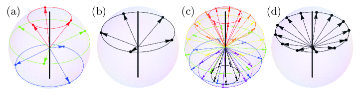
Figure 1: Reconstruction of spin-$j$ density matrices: $j=1$ (a, b) and $j=3$ (c, d). The procedure developed in [12] is represented by a and c; it is based on fixing $(2j+1)^{2}$ specifically arranged directions (32) and measuring the probabilities of the spin projection onto each direction to take the value $j$. The method used in [7] is illustrated by b and d; in this case, one needs to measure $4j+1$ spin-$j$ portraits ${\bf w}_{j}^{(j)}({\bf n}_{k})$, where ${\bf n}_{k}$ are specifically chosen to form a cone.

4 Quantum States as Probability Distributions

To begin, we showed in Sec. 2 that any quantum state can be interpreted as a probability distribution function. Since tomogram (1) is a function depending on the unitary matrix $u$ (direction ${\bf n}$ in the case of $u\in SU(2)$), there is a redundancy of information contained in the tomogram. It is tempting to reduce such a redundancy and associate a quantum state with the single probability distribution. The proposal to associate quantum states with single probability vectors was made in [21, 20, 18, 19, 17, 16]. To avoid any redundancy, it was suggested to use the minimum informationally complete POVM (positive operator-valued measure). This suggestion is related to constructing the minimum tomographic set discussed in [36]. Using the language of spin states, any spin-$j$ state is associated with the following $(2j+1)^{2}$-component probability vector:

$${\bf p}=\left(\begin{array}[]{c}{\rm tr}(\hat{\rho}\hat{E}_{1})\\ {\rm tr}(\hat{\rho}\hat{E}_{2})\\ \cdots\\ {\rm tr}(\hat{\rho}\hat{E}_{(2j+1)^{2}})\\ \end{array}\right),$$ (34)

where $\hat{E}_{i}$, $i=1,\dots,(2j+1)^{2}$ are the corresponding POVM effects. There are many ways to introduce the minimum informationally complete POVM effects, and a possible choice that is valid in any dimension was presented in [19]. A relatively new tendency is to use the symmetric informationally complete (SIC) POVMs. If this is the case, the effects $\{\hat{E}_{i}\}_{i=1}^{(2j+1)^{2}}$ are one-dimensional projectors satisfying the following condition:

$${\rm tr}(\hat{E}_{k}\hat{E}_{l})=\frac{1}{(2j+1)^{2}(2j+2)}\quad{\rm if}\quad k\neq l.$$ (35)

As stated in [20], the effects $\{\hat{E}_{i}\}_{i=1}^{(2j+1)^{2}}$ that meet the above requirements were found numerically in dimensions $(2j+1)\leq 67$ and analytically in dimensions $(2j+1)=2-15,~{}19,~{}{\rm and}~{}24$.

It is worth noting that the Amiet–Weigert construction considered in the previous section can be treated as a single probability distribution. For this, one needs to normalize vector (24). In this case, the mappings (29) and (31) are slightly modified

$${\bf W^{\prime}}=\frac{\|M\|\boldsymbol{\rho}}{\sum_{i,k=1}^{(2j+1)^{2}}\|M\|_{ik}\rho_{k}},\qquad\boldsymbol{\rho}=\frac{\|M\|^{-1}{\bf W^{\prime}}}{\sum_{i=1}^{2j+1}\sum_{k=1}^{(2j+1)^{2}}\|M\|_{(i-1)(2j+1)+i,k}^{-1}{W^{\prime}_{k}}}.$$ (36)

5 Inverse Spin-Portrait Method

In this section, starting from spin tomograms, we associate each quantum state with the corresponding probability distribution vector, which has a clear physical meaning and can be measured experimentally.

The unitary spin tomogram $w^{(j)}(m,u)$ is a function of the unitary matrix $u$ and depends on a discrete parameter $m=-j,\dots,j-1,j$. Fixing the unitary rotation $u_{k}$, we obtain a $(2j+1)$-component probability vector ${\bf w}_{j}^{(j)}(u_{k})$, called the spin-$j$ portrait of the system (see Sec. 2.1). Given only one spin-$j$ portrait of the system, it is impossible, in general, to define without doubt a state of the system. Nevertheless, the state is determined if one has an adequate number $N_{u}$ of different spin-$j$ portraits. Then we can introduce a joint probability distribution function of two random variables $m$ and $u_{k}$

$$\mathcal{P}(m,u_{k}),\qquad m=-j,-j+1,\dots,j,\quad k=1,2,\dots,N_{u}.$$ (37)

The physical meaning of this joint probability distribution is that, if one randomly chooses a unitary rotation from the set $\{u_{k}\}_{k=1}^{N_{u}}$ and a spin projection $m$ within the interval $-j\leq m\leq j$, the value of $\mathcal{P}(m,u_{k})$ gives the probability of the detector’s click. Function (37) can also be written in the form of the following $N_{u}(2j+1)$-component probability distribution vector:

$$\boldsymbol{\cal P}=\left(\begin{array}[]{cccccccccc}\mathcal{P}(j,u_{1})&\ldots&\mathcal{P}(-j,u_{1})&\mathcal{P}(j,u_{2})&\ldots&\mathcal{P}(-j,u_{2})&\ldots&\mathcal{P}(j,u_{N_{u}})&\ldots&\mathcal{P}(-j,u_{N_{u}})\\ \end{array}\right)^{T}$$ (39)

with the normalization condition of the form

$$\sum_{m=-j}^{j}\sum_{k=1}^{N_{u}}\mathcal{P}(m,u_{k})=1.$$ (41)

Since the tomogram $w^{(j)}(m,u_{k})$ is nothing else but the probability to obtain the spin projection $m$ if the rotation $u_{k}$ is fixed, the relation between the spin tomogram and the joint probability distribution function $\mathcal{P}(m,u_{k})$ reads

$$w^{(j)}(m,u_{k})=\frac{\mathcal{P}(m,u_{k})}{\sum_{m=-j}^{j}\mathcal{P}(m,u_{k})},$$ (42)

where the denominator has the sense of the probability $p_{k}$ to choose the unitary rotation $u_{k}$. If the probabilities $\{p_{k}\}_{k=1}^{N_{u}}$ are known a priori, then the vector $\boldsymbol{\cal P}$ is easily expressed via spin-$j$ portraits (11), namely,

$$\boldsymbol{\cal P}=\left(\begin{array}[]{c}p_{1}{\bf w}_{j}^{(j)}(u_{1})\\ p_{2}{\bf w}_{j}^{(j)}(u_{2})\\ \cdots\\ p_{N_{u}}{\bf w}_{j}^{(j)}(u_{N_{u}})\\ \end{array}\right).$$ (43)

If the unitary rotations $u_{k}$, $k=1,\dots,N_{u}$ are equiprobable, then

$$\boldsymbol{\cal P}_{\rm eq}=\frac{1}{N_{u}}\left(\begin{array}[]{c}{\bf w}_{j}^{(j)}(u_{1})\\ {\bf w}_{j}^{(j)}(u_{2})\\ \cdots\\ {\bf w}_{j}^{(j)}(u_{N_{u}})\\ \end{array}\right).$$ (44)

It is worth mentioning that, even if a priori the probabilities $\{p_{k}\}_{k=1}^{N_{u}}$ are not known, formula (42) provides a direct way of mapping $\boldsymbol{\cal P}$ onto the vector $\boldsymbol{\cal P}_{\rm eq}$.

Let us now consider an open problem of the minimum number $N_{u}$ of spin portraits. In other words, $N_{u}$ is the number of unitary rotations $u_{k}$ that is needed to identify any quantum state with a single probability vector of the form (43) and to minimize the redundancy of information contained in this vector. Subsequently, two main cases are presented, namely, the use of $SU(2)$ rotations and $SU(N)$ rotations with $N=2j+1$. These particular problems can be of interest for experimentalists because $SU(2)$ rotations can be relatively easily realized in some modifications of the Stern–Gerlach experiment, while $SU(N)$ rotations may require more difficult apparatus. On the other hand, it will be shown that, to extract information on the system, one can use a smaller number of $SU(N)$ rotations than in the case of $SU(2)$ matrices.

5.1 SU(2) Rotations

Like the Amiet–Weigert scanning procedure (29), the map of the density operator $\hat{\rho}$ onto the probability vector (43) can be written as follows:

$${\boldsymbol{\cal P}}=\|Q\|\boldsymbol{\rho},$$ (45)

where $\|Q\|$ is an $N_{u}(2j+1)\times(2j+1)^{2}$ rectangular matrix of the form

$$\|Q\|=\left(\begin{array}[]{c}p_{1}{\bf U}^{(j)}(j,{\bf n}_{1})^{T}\\ p_{1}{\bf U}^{(j)}(j-1,{\bf n}_{1})^{T}\\ \cdots\\ p_{1}{\bf U}^{(j)}(-j,{\bf n}_{1})^{T}\\ \vdots\\ p_{N_{u}}{\bf U}^{(j)}(j,{\bf n}_{N_{u}})^{T}\\ p_{N_{u}}{\bf U}^{(j)}(j-1,{\bf n}_{N_{u}})^{T}\\ \cdots\\ p_{N_{u}}{\bf U}^{(j)}(-j,{\bf n}_{N_{u}})^{T}\\ \end{array}\right).$$ (46)

The map (45) is invertible iff ${\rm rank}\|Q\|=(2j+1)^{2}$. Since the rank of a matrix is equal to the number of linearly independent rows, the number $N_{u}$ can be defined as the minimum natural number such that the set $\{{\bf U}^{(j)}(m,{\bf n}_{k})\}$, $m=-j,\dots,j$, $k=1,\dots,N_{u}$ contains $(2j+1)^{2}$ linearly independent vectors. According to [29], each vector ${\bf U}^{(j)}(m,{\bf n})$ can be resolved to the sum of orthogonal vectors ${\bf S}_{L}^{(j)}({\bf n})$, $L=0,\dots,2j$; namely,

$${\bf U}^{(j)}(m,{\bf n})=\sum_{L=0}^{2j}f_{L}^{(j)}(m){\bf S}_{L}^{(j)}({\bf n}),$$ (47)

where $\left({\bf S}_{L}^{(j)}({\bf n})\cdot{\bf S}_{L^{\prime}}^{(j)}({\bf n})\right)=\sum_{m=-j}^{j}f_{L}^{(j)}(m)f_{L^{\prime}}^{(j)}(m)=\delta_{LL^{\prime}}$. The vector ${\bf S}_{L}^{(j)}({\bf n})$ corresponds to the operator $\hat{S}_{L}^{(j)}({\bf n})$ acting on the Hilbert space of spin-$j$ states (see Sec. 2). The operator $\hat{S}_{L}^{(j)}({\bf n})$ is shown to be the same polynomial $f_{L}^{(j)}(m)$ of degree $L$, with the argument being replaced: $~{}m\longrightarrow(\hat{\bf J}\cdot{\bf n})=\hat{J}_{x}n_{x}+\hat{J}_{y}n_{y}+\hat{J}_{z}n_{z}$. Suppose $L=0$, then there exists only one linear independent vector of the form ${\bf S}_{L=0}^{(j)}({\bf n})$ which corresponds to the identity operator $\hat{I}$. If $L=1$, no more than three linear independent vectors ${\bf S}_{L=1}^{(j)}({\bf n}_{k})$, $k=1,2,3$, which correspond to the operators $(\hat{\bf J}\cdot{\bf n}_{1})$, $(\hat{\bf J}\cdot{\bf n}_{2})$, and $(\hat{\bf J}\cdot{\bf n}_{3})$, respectively, can exist. Note that the three vectors ${\bf S}_{L=1}^{(j)}({\bf n}_{k})$, $k=1,2,3$ are independent iff vectors ${\bf n}_{k}\in\mathbb{R}^{3}$ are not coplanar, i.e., their triple product $({\bf n}_{1}\cdot[{\bf n}_{2}\times{\bf n}_{3}])\neq 0$. Taking into account the normalization conditions ${\bf n}_{k}^{2}=1$ and $\hat{\bf J}^{2}=j(j+1)\hat{I}$, in the case $L=2$, we obtain five linear independent vectors ${\bf S}_{L=2}^{(j)}({\bf n}_{k})$. Using the matrix representation of the operator $\hat{S}_{L}^{(j)}({\bf n})$, we see that it is composed of $2L+1$ independent $l$-diagonal operators ($l=0$ for a diagonal one, $l=1$ for a super-diagonal one, $l=-1$ for a sub-diagonal one, and so on for all $-L\leq l\leq L$). Increasing $L$ by unity, two more diagonals are filled. We draw the conclusion that for a fixed $L$ the maximum number of linearly independent vectors ${\bf S}_{L}^{(j)}({\bf n}_{k})$ is equal to $2L+1$. Since vectors ${\bf S}_{L}^{(j)}({\bf n}_{k})$ and ${\bf S}_{L^{\prime}}^{(j)}({\bf n}_{k})$ with different $L$ and $L^{\prime}$ are orthogonal, the total number of linear independent rows ${\bf U}_{j}^{T}(m,{\bf n})$ equals $1+3+5+\dots+N_{u}=(N_{u}+1)^{2}/4$. On the other hand, it must be equal to ${\rm rank}\|Q\|=(2j+1)^{2}$. From this, it is readily seen that $N_{u}=4j+1$.

The directions ${\bf n}_{k}$, $k=1,\dots,4j+1$ cannot be chosen arbitrarily because of the condition ${\rm rank}\|Q\|=(2j+1)^{2}$. As was shown above, the directions $\{{\bf n}_{k}\}_{k=1}^{4j+1}$ are divided into sets of one, three, five, and so on directions. Without loss of generality, it can be assumed that these sets are $\{{\bf n}_{1}\}$, $\{{\bf n}_{k}\}_{k=1}^{3}$, $\{{\bf n}_{k}\}_{k=1}^{5}$, $\dots$, $\{{\bf n}_{k}\}_{k=1}^{4j+1}$, respectively. If this is the case, the requirement ${\rm rank}\|Q\|=(2j+1)^{2}$ is equivalent to the condition

$$\Delta_{1}\Delta_{2}\cdot\ldots\cdot\Delta_{2j}\neq 0,$$ (48)

where $\Delta_{q}$, $q=1,\dots,2j$ are expressed through ${\bf n}_{k}=(\sin\theta_{k}\cos\varphi_{k},\sin\theta_{k}\sin\varphi_{k},\cos\theta_{k})$ and associated Legendre polynomials $P_{l}^{(m)}(x)$ as follows:

$$\Delta_{q}=\det\left(\begin{array}[]{cccc}P_{q}^{(0)}(\cos\theta_{1})&\cdots&P_{q}^{(q)}(\cos\theta_{1})\cos q\varphi_{1}&P_{q}^{(q)}(\cos\theta_{1})\sin q\varphi_{1}\\ P_{q}^{(0)}(\cos\theta_{2})&\cdots&P_{q}^{(q)}(\cos\theta_{2})\cos q\varphi_{2}&P_{q}^{(q)}(\cos\theta_{2})\sin q\varphi_{2}\\ P_{q}^{(0)}(\cos\theta_{3})&\cdots&P_{q}^{(q)}(\cos\theta_{3})\cos q\varphi_{3}&P_{q}^{(q)}(\cos\theta_{3})\sin q\varphi_{3}\\ \cdots&\cdots&\cdots&\cdots\\ P_{q}^{(0)}(\cos\theta_{2q})&\cdots&P_{q}^{(q)}(\cos\theta_{2q})\cos q\varphi_{2q}&P_{q}^{(q)}(\cos\theta_{2q})\sin q\varphi_{2q}\\ P_{q}^{(0)}(\cos\theta_{2q+1})&\cdots&P_{q}^{(q)}(\cos\theta_{2q+1})\cos q\varphi_{2q+1}&P_{q}^{(q)}(\cos\theta_{2q+1})\sin q\varphi_{2q+1}\\ \end{array}\right).$$ (49)

In the particular case of $q=1$, we have

$$\Delta_{1}=\det\left(\begin{array}[]{ccc}P_{1}^{(0)}(\cos\theta_{1})&P_{1}^{(1)}(\cos\theta_{1})\cos\varphi_{1}&P_{1}^{(1)}(\cos\theta_{1})\sin\varphi_{1}\\ P_{1}^{(0)}(\cos\theta_{2})&P_{1}^{(1)}(\cos\theta_{2})\cos\varphi_{2}&P_{1}^{(1)}(\cos\theta_{2})\sin\varphi_{2}\\ P_{1}^{(0)}(\cos\theta_{3})&P_{1}^{(1)}(\cos\theta_{3})\cos\varphi_{3}&P_{1}^{(1)}(\cos\theta_{3})\sin\varphi_{3}\\ \end{array}\right)=({\bf n}_{1}\cdot[{\bf n}_{2}\times{\bf n}_{3}]).$$ (50)

It is worth mentioning that there exists an optimum choice of the directions $\{{\bf n}_{k}\}_{k=1}^{4j+1}$ that provides minimum possible errors of the reconstruction procedure due to errors in measured probabilities ${\cal P}(m,{\bf n}_{k})$. Indeed, according to the results of computational mathematics (see, e.g., [35]), the errors of the vector $\boldsymbol{\rho}$ defined by formula (45) are directly proportional to the condition number $\mu(Q)$ of the matrix $\|Q\|$. The greater the product $\Delta_{1}\cdot\ldots\cdot\Delta_{2j}$, the smaller $\mu(Q)$ and, consequently, the errors of the reconstruction procedure. For qubits ($j=1/2$), the optimum choice is three orthogonal vectors $\{{\bf n}_{k}\}_{k=1}^{3}$ because their triple product takes the maximum value in this case. As far as higher spins are concerned, maximization of expression (48) is performed numerically, and the optimum directions $\{{\bf n}_{k}\}_{k=1}^{(4j+1)}$ are shown in Fig. 2.

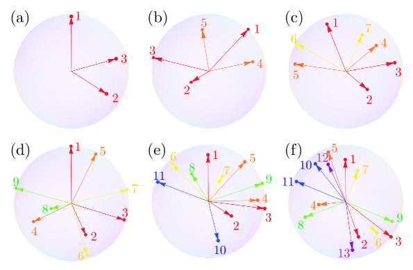
Figure 2: Optimum choice of the directions $\{{\bf n}_{k}\}_{k=1}^{4j+1}$ that ensures the minimum possible errors of the density operator $\hat{\rho}$ with respect to the errors of the probability vector $\boldsymbol{\cal P}$, where $j=1/2$ (a), $j=1$ (b), $j=3/2$ (c), $j=2$ (d), $j=5/2$ (e), and $j=3$ (f).

A particular case of $\theta_{1}=\theta_{2}=\ldots=\theta_{4j+1}=\theta$ corresponds to the Newton–Young reconstruction procedure [7] and implies the limitation $P_{L}^{(m)}(\cos\theta)\neq 0$ for all $0\leq m\leq L$, $1\leq L\leq 2j$. A schematic illustration of this reconstruction procedure is given in Fig. 1.

An alternative way to meet the requirement ${\rm rank}\|Q\|=(2j+1)^{2}$ is to ensure linear independence of vectors $\{{\bf S}_{L}^{(j)}({\bf n}_{k})\}_{k=1}^{2L+1}$ for all $L=1,\dots,2j$. Linear independence of these vectors is equivalent to nonzero Gram determinant $\det\left\|\Big{(}{\bf S}_{L}^{(j)}({\bf n}_{i})\cdot{\bf S}_{L}^{(j)}({\bf n}_{k})\Big{)}\right\|_{i,k=1}^{2L+1}$. Since $\Big{(}{\bf S}_{L}^{(j)}({\bf n}_{i})\cdot{\bf S}_{L}^{(j)}({\bf n}_{k})\Big{)}=P_{L}^{(0)}({\bf n}_{i}\cdot{\bf n}_{k})$, we obtain

$$\det\left\|P_{1}^{(0)}({\bf n}_{i}\cdot{\bf n}_{k})\right\|_{i,k=1}^{3}\cdot\det\left\|P_{2}^{(0)}({\bf n}_{i}\cdot{\bf n}_{k})\right\|_{i,k=1}^{5}\cdot\ldots\cdot\det\left\|P_{2j}^{(0)}({\bf n}_{i}\cdot{\bf n}_{k})\right\|_{i,k=1}^{4j+1}\neq 0.$$ (51)

In the case of qubits, one has

$$\Delta_{1}^{\prime}=\det\left(\begin{array}[]{ccc}({\bf n}_{1}\cdot{\bf n}_{1})&({\bf n}_{1}\cdot{\bf n}_{2})&({\bf n}_{1}\cdot{\bf n}_{3})\\ ({\bf n}_{2}\cdot{\bf n}_{1})&({\bf n}_{2}\cdot{\bf n}_{2})&({\bf n}_{2}\cdot{\bf n}_{3})\\ ({\bf n}_{3}\cdot{\bf n}_{1})&({\bf n}_{3}\cdot{\bf n}_{2})&({\bf n}_{3}\cdot{\bf n}_{3})\\ \end{array}\right)=({\bf n}_{1}\cdot[{\bf n}_{2}\times{\bf n}_{3}])^{2}\neq 0.$$ (52)

As far as qutrits ($j=1$) are concerned, we obtain

$$\Delta_{1}^{\prime}\!\cdot\!\det\!\left(\begin{array}[]{ccccc}1&\frac{3({\bf n}_{1}\cdot{\bf n}_{2})^{2}-1}{2}&\frac{3({\bf n}_{1}\cdot{\bf n}_{3})^{2}-1}{2}&\frac{3({\bf n}_{1}\cdot{\bf n}_{4})^{2}-1}{2}&\frac{3({\bf n}_{1}\cdot{\bf n}_{5})^{2}-1}{2}\\ \frac{3({\bf n}_{2}\cdot{\bf n}_{1})^{2}-1}{2}&1&\frac{3({\bf n}_{2}\cdot{\bf n}_{3})^{2}-1}{2}&\frac{3({\bf n}_{2}\cdot{\bf n}_{4})^{2}-1}{2}&\frac{3({\bf n}_{2}\cdot{\bf n}_{5})^{2}-1}{2}\\ \frac{3({\bf n}_{3}\cdot{\bf n}_{1})^{2}-1}{2}&\frac{3({\bf n}_{3}\cdot{\bf n}_{2})^{2}-1}{2}&1&\frac{3({\bf n}_{3}\cdot{\bf n}_{4})^{2}-1}{2}&\frac{3({\bf n}_{3}\cdot{\bf n}_{5})^{2}-1}{2}\\ \frac{3({\bf n}_{4}\cdot{\bf n}_{1})^{2}-1}{2}&\frac{3({\bf n}_{4}\cdot{\bf n}_{2})^{2}-1}{2}&\frac{3({\bf n}_{4}\cdot{\bf n}_{3})^{2}-1}{2}&1&\frac{3({\bf n}_{4}\cdot{\bf n}_{5})^{2}-1}{2}\\ \frac{3({\bf n}_{5}\cdot{\bf n}_{1})^{2}-1}{2}&\frac{3({\bf n}_{5}\cdot{\bf n}_{2})^{2}-1}{2}&\frac{3({\bf n}_{5}\cdot{\bf n}_{3})^{2}-1}{2}&\frac{3({\bf n}_{5}\cdot{\bf n}_{4})^{2}-1}{2}&1\\ \end{array}\right)\!\neq\!0.$$ (53)

5.2 SU(N) Rotations in Hilbert Space

If the matrix $u$ in the definition of spin tomogram $w^{(j)}(m,u)$ is an element of the group $SU(N)$ with $2<N\leq 2j+1$, the tomogram $w^{(j)}(m,u)$ is also referred to as a unitary spin tomogram [22]. The case $N=2j+1$ corresponds to the most general form of unitary rotations in the Hilbert space of spin $j$. By the previous statement, we can assume linear independence of vectors $\{{\bf U}(m,u_{k})\}$, where the spin projection $m$ takes values $m=-j,-j+1,\dots,j-1$ and $k$ runs from $1$ to $N_{u}$. Here $N_{u}$ denotes the minimum number of spin portraits ${\bf w}_{j}^{(j)}(u_{k})$, $u_{k}\in SU(N)$, $N=2j+1$, that are needed to construct a bijective map. Since $\sum_{m=-j}^{j}\hat{U}^{(j)}(m,u_{k})=\hat{I}$ for all $k=1,\dots,N_{u}$, we have one more independent vector. Thus, the total number of linear independent vectors $\{{\bf U}(m,u_{k})\}$ equals $2jN_{u}+1$. On the other hand, this number must be equal to $(2j+1)^{2}$ for the map to be invertible. Consequently, $N_{u}=((2j+1)^{2}-1)/2j=2j+2$.

We see that one needs fewer $SU(N)$ rotations than $SU(2)$ rotations in order to map a quantum state onto a single probability distribution. Nevertheless, this advantage is accompanied by the complexity of the experimental realization of $SU(N)$ rotations with regard to $SU(2)$ rotations in the Hilbert space. For intermediate cases $2<N<2j+1$, we have $2j+2\leq N_{u}<4j+1$.

Let us consider the case of $SU(N)$ rotations with $N=2j+1$ in detail. As in the previous section, any quantum state is mapped onto a single $(2j+1)(2j+2)$-probability vector $\boldsymbol{\cal P}$ as follows:

$${\boldsymbol{\cal P}}=\|R\|\boldsymbol{\rho},$$ (54)

where the $(2j+1)(2j+2)\times(2j+1)^{2}$ rectangular matrix $\|R\|$ reads

$$\|R\|=\left(\begin{array}[]{c}p_{1}{\bf U}^{(j)}(j,u_{1})^{T}\\ p_{1}{\bf U}^{(j)}(j-1,u_{1})^{T}\\ \cdots\\ p_{1}{\bf U}^{(j)}(-j,u_{1})^{T}\\ \vdots\\ p_{2j+2}{\bf U}^{(j)}(j,u_{2j+2})^{T}\\ p_{2j+2}{\bf U}^{(j)}(j-1,u_{2j+2})^{T}\\ \cdots\\ p_{2j+2}{\bf U}^{(j)}(-j,u_{2j+2})^{T}\\ \end{array}\right).$$ (55)

Taking into account the condition ${\rm rank}\|R\|=(2j+1)^{2}$, we express the inverse map $\boldsymbol{\cal P}\rightarrow\boldsymbol{\rho}$ through a pseudo-inverse matrix $\|R^{+}\|$ [37] as follows:

$$\boldsymbol{\rho}=\|R^{+}\|\boldsymbol{\cal P}=\left(\|R^{{\dagger}}\|\|R\|\right)^{-1}\|R^{{\dagger}}\|\boldsymbol{\cal P}.$$ (56)

The requirement ${\rm rank}\|R\|=(2j+1)^{2}$ is equivalent to the linear independence of vectors ${\bf U}^{(j)}(m,u_{k})$, $m=-j,-j+1,\dots,j-1$, $k=1,2,\dots,2j+2$ and the vector ${\bf I}=\sum_{m=-j}^{j}{\bf U}^{(j)}(m,u_{k})$, which does not rely on $k$. The linear independence of these vectors is achieved whenever the corresponding Gram determinant is nonzero. That yields the constraint of the form

$$\Gamma=\det\left(\begin{array}[]{c|c|c|c|c}2j+1&1\ 1\ \dots\ 1&1\ 1\ \dots\ 1&\cdots&1\ 1\ \dots\ 1\\ \hline\cr\begin{smallmatrix}1\\ 1\\ \cdots\\ 1\end{smallmatrix}&I_{2j}&\Lambda(u_{1}u_{2}^{{\dagger}})&\cdots&\Lambda(u_{1}u_{2j+2}^{{\dagger}})\\ \hline\cr\begin{smallmatrix}1\\ 1\\ \cdots\\ 1\end{smallmatrix}&\Lambda(u_{2}u_{1}^{{\dagger}})&I_{2j}&\cdots&\Lambda(u_{2}u_{2j+2}^{{\dagger}})\\ \hline\cr\cdots&\cdots&\cdots&\cdots&\cdots\\ \hline\cr\begin{smallmatrix}1\\ 1\\ \cdots\\ 1\end{smallmatrix}&\Lambda(u_{2j+2}u_{1}^{{\dagger}})&\Lambda(u_{2j+2}u_{2}^{{\dagger}})&\cdots&I_{2j}\\ \end{array}\right)\neq 0,$$ (57)

where the Gram matrix is composed of blocks: $~{}I_{2j}$ is the $2j\times 2j$ unity matrix and $\Lambda(u_{k}u_{k^{\prime}}^{{\dagger}})$ is a $2j\times 2j$ matrix with elements $\|\Lambda(u_{k}u_{k^{\prime}}^{{\dagger}})\|_{ln}=|\langle jl|u_{k}u_{k^{\prime}}^{{\dagger}}|jn\rangle|^{2}$. Using the orthogonal expansion of dequantizer (5), we rewrite the condition obtained in terms of vectors ${\bf S}_{L}^{(j)}(u_{k})$ as follows:

$$\Gamma^{\prime}=\det\left(\begin{array}[]{c|c|c|c}I_{2j}&\Lambda^{\prime}(u_{1},u_{2})&\cdots&\Lambda^{\prime}(u_{1},u_{2j+2})\\ \hline\cr\Lambda^{\prime}(u_{2},u_{1})&I_{2j}&\cdots&\Lambda^{\prime}(u_{2},u_{2j+2})\\ \hline\cr\cdots&\cdots&\cdots&\cdots\\ \hline\cr\Lambda^{\prime}(u_{2j+2},u_{1})&\Lambda^{\prime}(u_{2j+2},u_{2})&\cdots&I_{2j}\\ \end{array}\right)\neq 0,$$ (58)

where $\Lambda^{\prime}(u_{k},u_{k^{\prime}})$ is a $2j\times 2j$ matrix with elements $\|\Lambda^{\prime}(u_{k},u_{k^{\prime}})\|_{LL^{\prime}}=\Big{(}{\bf S}_{L}^{(j)}(u_{k})\cdot{\bf S}_{L^{\prime}}^{(j)}(u_{k^{\prime}})\Big{)}$. Note that $\Gamma^{\prime}$ is nothing else but the volume of the $2j(2j+2)$-dimensional parallelogram with edges ${\bf S}_{L}^{(j)}(u_{k})$, $L=1,\dots,2j$, $k=1,\dots,2j+2$. Moreover, $0\leq\Gamma^{\prime}\leq 1$ since all vectors ${\bf S}_{L}^{(j)}(u_{k})$ are normalized.

The optimum choice of unitary matrices $u_{k}\in SU(N)$, $N=2j+1$, follows the same line of reasoning as in the case of $SU(2)$ rotations. Indeed, if the probability vector $\boldsymbol{\cal P}$ is measured experimentally within the accuracy $\delta\boldsymbol{\cal P}$, formula (56) yields the vector $\boldsymbol{\rho}$ defined with an error bar of $\delta\boldsymbol{\rho}$. It is known that $\frac{\|\delta\boldsymbol{\rho}\|_{2}}{\|\boldsymbol{\rho}\|_{2}}\leq\mu\frac{\|\delta\boldsymbol{\cal P}\|_{2}}{\|\boldsymbol{\cal P}\|_{2}}$, where $\mu$ is the condition number of the matrix (58) and $\|\cdot\|_{2}$ is the Euclidean norm of a vector. It can be shown that $\mu\leq\frac{1+\sqrt{1-\Gamma^{\prime}}}{1-\sqrt{1-\Gamma^{\prime}}}$. Consequently, the greater $\Gamma^{\prime}$ (or $\Gamma$), the less erroneous is the reconstructed state $\boldsymbol{\rho}$.

6 Inverse Mapping of a Probability Vector onto the Density Matrix

In this section, we give an explicit expression of the density operator $\hat{\rho}$ of the system with spin $j$ in terms of the single probability vector $\boldsymbol{\cal P}$, which could itself be treated as the notion of quantum state. We consider distributions $\boldsymbol{\cal P}$ obtained by $SU(2)$ rotations. It was shown in Sec. 5 that any vector $\boldsymbol{\cal P}$ is readily transformed into the vector $\boldsymbol{\cal P}_{\rm eq}$. For this reason, we will focus attention on the map $\boldsymbol{\cal P}_{\rm eq}\rightarrow\hat{\rho}$.

Let us now recall that the direct map reads

$${\cal P}_{\rm eq}(m,{\bf n}_{k})=\frac{1}{4j+1}w^{(j)}(m,{\bf n}_{k})=\frac{1}{4j+1}{\rm Tr}\Big{(}\hat{\rho}~{}\hat{U}^{(j)}(m,{\bf n}_{k})\Big{)},$$ (59)

where $\hat{U}^{(j)}(m,{\bf n}_{k})$ is the dequantizer operator that can be resolved into sum (4). This means that

$${\cal P}_{\rm eq}(m,{\bf n}_{k})=\frac{1}{4j+1}w^{(j)}(m,{\bf n}_{k})=\frac{1}{4j+1}\sum_{L=0}^{2j}f_{L}^{(j)}(m){\rm Tr}\Big{(}\hat{\rho}\hat{S}_{L}^{(j)}({\bf n}_{k})\Big{)}=\sum_{L=0}^{2j}{\rm Tr}\Big{(}\hat{\rho}~{}\hat{\cal U}_{L}^{(j)}(m,{\bf n}_{k})\Big{)},$$

where we introduce the $L$-dequantizer operator $\hat{\cal U}_{L}^{(j)}(m,{\bf n}_{k})=(4j+1)^{-1}f_{L}^{(j)}(m)\hat{S}_{L}^{(j)}({\bf n}_{k})$.

Since the direct map is linear, it can be assumed that the inverse map is also linear, that is,

$$\hat{\rho}=\sum_{k=1}^{4j+1}\sum_{m=-j}^{j}{\cal P}_{\rm eq}(m,{\bf n}_{k})\hat{\cal D}^{(j)}(m,k),$$ (61)

where $\hat{\cal D}^{(j)}(m,k)$ is the quantizer operator to be determined. We already know that it is convenient to rearrange directions $\{{\bf n}_{k}\}_{k=1}^{4j+1}$ and consider sets $\{{\bf n}_{k}\}_{k=1}^{2L+1}$, $L=0,1,\dots,2j$. In view of this fact, we treat a solution of the form

$$\hat{\rho}=\sum_{L=0}^{2j}\sum_{k=1}^{2L+1}\sum_{m=-j}^{j}{\cal P}_{\rm eq}(m,{\bf n}_{k})\hat{\cal D}_{L}^{(j)}(m,k).$$ (62)

If $L$-quantizers $\hat{\cal D}_{L}^{(j)}(m,k)$ are known, we immediately have $\hat{\cal D}^{(j)}(m,k)=\sum\limits_{L:~{}(k-1)/2\leq L\leq 2j}\hat{\cal D}_{L}^{(j)}(m,k)$.

Proposition. The $L$-quantizer is expressed through operators $\hat{S}_{L}^{(j)}({\bf n}_{k^{\prime}})$ and Gram matrix $\|\mathscr{M}(L)\|$, whose matrix elements are $\|\mathscr{M}(L)\|_{kk^{\prime}}={\rm Tr}\left(\hat{S}_{L}^{(j)}({\bf n}_{k})\hat{S}_{L}^{(j)}({\bf n}_{k^{\prime}})\right)=\left({\bf S}_{L}^{(j)}({\bf n}_{k})\cdot{\bf S}_{L}^{(j)}({\bf n}_{k^{\prime}})\right)=P_{L}({\bf n}_{k}\cdot{\bf n}_{k^{\prime}})$, as follows:

$$\hat{\cal D}_{L}^{(j)}(m,k)=(4j+1)f_{L}^{(j)}(m)\sum_{k^{\prime}=1}^{2L+1}\|\mathscr{M}^{-1}(L)\|_{kk^{\prime}}\hat{S}_{L}^{(j)}({\bf n}_{k^{\prime}}),$$ (63)

with the operators $\left\{\sum_{k^{\prime}=1}^{2L+1}\|\mathscr{M}^{-1}(L)\|_{kk^{\prime}}\hat{S}_{L}^{(j)}({\bf n}_{k^{\prime}})\right\}_{k=1}^{2L+1}$ forming a dual basis for the given basis
$\left\{\hat{S}_{L}^{(j)}({\bf n}_{k})\right\}_{k=1}^{2L+1}$.

$\square$

Let us check that formula (63) gives an adequate solution of the problem.

If the directions $\{{\bf n}_{k}\}_{k=1}^{2j+1}$ are chosen properly and the requirement (48) is satisfied (which is equivalent to $\prod_{L=1}^{2j}\det\|\mathscr{M}(L)\|\neq 0$), then any density operator $\hat{\rho}$ is resolved into a sum of orthogonal operators

$$\hat{\rho}=\sum_{L^{\prime}=0}^{2j}\sum_{k^{\prime}=1}^{2L^{\prime}+1}a(L^{\prime},k^{\prime})\hat{S}_{L^{\prime}}^{(j)}({\bf n}_{k^{\prime}}).$$ (64)

Substituting formula (64) for $\hat{\rho}$ in (6), we obtain

$${\rm Tr}\Big{(}\hat{\rho}\hat{S}_{L}^{(j)}({\bf n}_{k})\Big{)}=\sum_{L^{\prime}=0}^{2j}\sum_{k^{\prime}=1}^{2L^{\prime}+1}a(L^{\prime},k^{\prime}){\rm Tr}\Big{(}\hat{S}_{L^{\prime}}^{(j)}({\bf n}_{k^{\prime}})\hat{S}_{L}^{(j)}({\bf n}_{k})\Big{)}=\sum_{k^{\prime}=1}^{2L+1}a(L,k^{\prime})\|\mathscr{M}(L)\|_{kk^{\prime}},$$ (65)

$${\cal P}_{\rm eq}(m,{\bf n}_{k})=\frac{1}{4j+1}\sum_{L=0}^{2j}f_{L}^{(j)}(m)\sum_{k^{\prime}=1}^{2L+1}a(L,k^{\prime})\|\mathscr{M}(L)\|_{kk^{\prime}}.$$ (66)

After combining (63) and (66), direct calculation of the right-hand side of Eq. (62) yields

$$\sum_{L=0}^{2j}\sum_{k=1}^{2L+1}\sum_{m=-j}^{j}{\cal P}_{\rm eq}(m,{\bf n}_{k})\hat{\cal D}_{L}^{(j)}(m,k)$$

$$=\sum_{L,L^{\prime\prime}=0}^{2j}\sum_{k,k^{\prime\prime}=1}^{2L+1}\sum_{k^{\prime}=1}^{2L^{\prime\prime}+1}\bigg{[}\underbrace{\sum_{m=-j}^{j}f_{L^{\prime\prime}}^{(j)}(m)f_{L}^{(j)}(m)}_{\delta_{L^{\prime\prime}L}}\bigg{]}a(L^{\prime\prime},k^{\prime})\|\mathscr{M}(L^{\prime\prime})\|_{kk^{\prime}}\|\mathscr{M}^{-1}(L)\|_{kk^{\prime\prime}}\hat{S}_{L}^{(j)}({\bf n}_{k^{\prime}})$$

$$=\sum_{L=0}^{2j}\sum_{k^{\prime},k^{\prime\prime}=1}^{2L+1}a(L,k^{\prime})\bigg{[}\underbrace{\sum_{k=1}^{2L+1}\|\mathscr{M}(L)\|_{kk^{\prime}}\|\mathscr{M}^{-1}(L)\|_{kk^{\prime\prime}}}_{\delta_{k^{\prime}k^{\prime\prime}}}\bigg{]}\hat{S}_{L}^{(j)}({\bf n}_{k^{\prime}})=\sum_{L=0}^{2j}\sum_{k^{\prime}=1}^{2L+1}a(L,k^{\prime})\hat{S}_{L}^{(j)}({\bf n}_{k^{\prime}})=\hat{\rho}.$$

This concludes the proof.

$\blacksquare$

In fact, the proof above is followed by the relation between the $L$-dequantizer and the $L^{\prime}$-quantizer

$${\rm Tr}\left(\hat{\cal U}_{L}^{(j)}(m,{\bf n}_{k})\hat{\cal D}_{L^{\prime}}^{(j)}(m^{\prime},{\bf n}_{k^{\prime}})\right)=f_{L}^{(j)}(m)f_{L}^{(j)}(m^{\prime})\delta_{LL^{\prime}}\delta_{kk^{\prime}}.$$ (68)

To summarize the results of this section, we write the explicit form of the quantizer

$$\hat{\cal D}^{(j)}(m,k)=\sum\limits_{L:~{}(k-1)/2\leq L\leq 2j}\hat{\cal D}_{L}^{(j)}(m,k)=(4j+1)\sum\limits_{L:~{}(k-1)/2\leq L\leq 2j}f_{L}^{(j)}(m)\sum_{k^{\prime}=1}^{2L+1}\|\mathscr{M}^{-1}(L)\|_{kk^{\prime}}\hat{S}_{L}^{(j)}({\bf n}_{k^{\prime}}).$$ (69)

7 Star-Product and Intertwining Kernels

Suppose ${\cal P}_{{\rm eq}~{}i}(m_{i},{\bf n}_{k_{i}})$ is the symbol (59) of a state $\hat{\rho}_{i}$, $i=1,2$; then the operator $\hat{\rho}_{1}\hat{\rho}_{2}$ is associated with a symbol ${\cal P}_{{\rm eq}~{}3}(m_{3},{\bf n}_{k_{3}})$ which is called the star product [38, 39, 40] of symbols ${\cal P}_{{\rm eq}~{}1}(m_{1},{\bf n}_{k_{1}})$ and ${\cal P}_{{\rm eq}~{}2}(m_{2},{\bf n}_{k_{2}})$ and denoted by $({\cal P}_{{\rm eq}~{}1}\star{\cal P}_{{\rm eq}~{}2})(m_{3},{\bf n}_{k_{3}})$. Combining (6) and (69), it is not hard to see that

$${\cal P}_{{\rm eq}~{}3}(m_{3},{\bf n}_{k_{3}})=\sum_{k_{1},k_{2}=1}^{4j+1}\sum_{m_{1},m_{2}=-j}^{j}K^{(j)}(m_{3},{\bf n}_{k_{3}},m_{2},{\bf n}_{k_{2}},m_{1},{\bf n}_{k_{1}}){\cal P}_{{\rm eq}~{}2}(m_{2},{\bf n}_{k_{2}}){\cal P}_{{\rm eq}~{}1}(m_{1},{\bf n}_{k_{1}}),$$

where the star-product kernel $K^{(j)}(m_{3},{\bf n}_{k_{3}},m_{2},{\bf n}_{k_{2}},m_{1},{\bf n}_{k_{1}})$ reads

$$K^{(j)}(m_{3},{\bf n}_{k_{3}},m_{2},{\bf n}_{k_{2}},m_{1},{\bf n}_{k_{1}})={\rm Tr}\left[\hat{\cal D}^{(j)}(m_{1},{n}_{k_{1}})\hat{\cal D}^{(j)}(m_{2},{n}_{k_{2}})\hat{\cal U}^{(j)}(m_{3},{n}_{k_{3}})\right]$$

$$=(4j+1)\sum\limits_{\{L_{1}:~{}(k_{1}-1)/2\leq L_{1}\leq 2j\}}\sum\limits_{\{L_{2}:~{}(k_{2}-1)/2\leq L_{2}\leq 2j\}}\sum_{L_{3}=0}^{2j}f_{L_{1}}^{(j)}(m_{1})f_{L_{2}}^{(j)}(m_{2})f_{L_{3}}^{(j)}(m_{3})$$

$$\quad\times\sum_{k_{1}^{\prime}=1}^{2L_{1}+1}\sum_{k_{2}^{\prime}=1}^{2L_{2}+1}\|\mathscr{M}^{-1}(L_{1})\|_{k_{1}k_{1}^{\prime}}\|\mathscr{M}^{-1}(L_{2})\|_{k_{2}k_{2}^{\prime}}{\rm Tr}\left[\hat{S}_{L_{1}}^{(j)}({\bf n}_{k_{1}^{\prime}})\hat{S}_{L_{2}}^{(j)}({\bf n}_{k_{2}^{\prime}})\hat{S}_{L_{3}}^{(j)}({\bf n}_{k_{3}})\right].$$ (71)

Let us recall that we have considered previously two maps of the density operator $\hat{\rho}$ onto the probability distribution functions, namely, the map onto tomograms $w^{(j)}(m,{\bf n})$ depending on the continuous variable ${\bf n}={\bf n}(\theta,\varphi)\in S^{2}$ and the map onto the single probability distribution ${\cal P}_{\rm eq}(m,{\bf n}_{k})$ depending on the discrete variable ${\bf n}_{k}$, $k=1,2,\dots,4j+1$. Since both maps are invertible, symbols $w^{(j)}(m,{\bf n})$ and ${\cal P}_{\rm eq}(m,{\bf n}_{k})$ are related by intertwining kernels. Indeed, combining formulas (3) and (59), we obtain

$${\cal P}_{\rm eq}(m,{\bf n}_{k})=\sum_{m^{\prime}=-j}^{j}\int\limits_{S^{2}}\frac{d{\bf n}^{\prime}}{4\pi}K_{w\rightarrow{\cal P}}^{(j)}(m,{\bf n}_{k},m^{\prime},{\bf n}^{\prime})w^{(j)}(m^{\prime},{\bf n}^{\prime}),$$ (72)

where $K_{w\rightarrow{\cal P}}^{(j)}(m,{\bf n}_{k},m^{\prime},{\bf n}^{\prime})=(4j+1)^{-1}{\rm Tr}\left(\hat{D}^{(j)}(m^{\prime},{\bf n}^{\prime})\hat{U}^{(j)}(m,{\bf n}_{k})\right)$. Using expansions (4) and (5) along with the orthogonality property ${\rm Tr}\left(\hat{S}_{L^{\prime}}({\bf n}^{\prime})\hat{S}_{L}({\bf n}_{k})\right)=\delta_{LL^{\prime}}P_{L}({\bf n}^{\prime}\cdot{\bf n}_{k})$, we arrive at

$$K_{w\rightarrow{\cal P}}^{(j)}(m,{\bf n}_{k},m^{\prime},{\bf n}^{\prime})=(4j+1)^{-1}\sum_{L=0}^{2j}(2L+1)f_{L}^{(j)}(m^{\prime})f_{L}^{(j)}(m)P_{L}({\bf n}^{\prime}\cdot{\bf n}_{k}).$$ (73)

In view of the same argument, the tomogram $w^{(j)}(m,{\bf n})$ is expressed through the joint probability distribution ${\cal P}_{\rm eq}(m^{\prime},{\bf n}_{k^{\prime}})$ as follows:

$$w^{(j)}(m,{\bf n})=\sum_{k^{\prime}=1}^{4j+1}\sum_{m^{\prime}=-j}^{j}K_{{\cal P}\rightarrow w}^{(j)}(m,{\bf n},m^{\prime},k^{\prime}){\cal P}_{\rm eq}(m^{\prime},{\bf n}_{k^{\prime}}),$$ (74)

where $K_{{\cal P}\rightarrow w}^{(j)}(m,{\bf n},m^{\prime},k^{\prime})={\rm Tr}\left(\hat{\cal D}^{(j)}(m^{\prime},k^{\prime})\hat{U}^{(j)}(m,{\bf n})\right)$. Taking into account explicit formula (69), we obtain

$$K_{{\cal P}\rightarrow w}^{(j)}(m,{\bf n},m^{\prime},k^{\prime})=(4j+1)\sum\limits_{L:~{}(k^{\prime}-1)/2\leq L\leq 2j}f_{L}^{(j)}(m^{\prime})f_{L}^{(j)}(m)\sum_{k=1}^{2L+1}\|\mathscr{M}^{-1}(L)\|_{k^{\prime}k}P_{L}({\bf n}_{k}\cdot{\bf n}).$$ (75)

8 Examples: Qubits and Qutrits

In this section, the results of the previous sections are specified for two particular cases of lowest spins, namely, qubits ($j=1/2$) and qutrits ($j=1$). As far as qubits are concerned, only the $SU(2)$ rotations are possible. A quantum state is associated with the six-dimensional probability vector $\boldsymbol{\cal P}$ with components ${\cal P}(m,{\bf n}_{k})$, $m=\pm 1/2$ and $k=1,2,3$. In other words, the probability vector $\boldsymbol{\cal P}$ is composed of three qubit portraits defined by directions $\{{\bf n}_{k}\}_{k=1}^{3}$. If these directions are equiprobable (chosen with the same probability $p_{k}=1/3$), the corresponding probability vector is denoted as $\boldsymbol{\cal P}_{\rm eq}$. Note that formula (42) defines the mapping $\boldsymbol{\cal P}\rightarrow\boldsymbol{\cal P}_{\rm eq}$ for any vector $\boldsymbol{\cal P}$. For the map $\hat{\rho}\rightarrow\boldsymbol{\cal P}$ to be invertible, the limitation $({\bf n}_{1}\cdot[{\bf n}_{2}\times{\bf n}_{3}])\neq 0$ is imposed. The least erroneous reconstruction procedure (see Fig. 2) takes place if all three directions are orthogonal, i.e., $({\bf n}_{1}\cdot[{\bf n}_{2}\times{\bf n}_{3}])=\pm 1$. In general, the inverse map (62) of the probability vector $\boldsymbol{\cal P}_{\rm eq}$ onto the density operator $\hat{\rho}$ reads

$$\hat{\rho}=\frac{1}{2}\left[{\cal P}_{\rm eq}(+1/2,{\bf n}_{1})+{\cal P}_{\rm eq}(-1/2,{\bf n}_{1})\right]\hat{I}+\sum_{k=1}^{3}\left[{\cal P}_{\rm eq}(+1/2,{\bf n}_{k})-{\cal P}_{\rm eq}(-1/2,{\bf n}_{k})\right](\hat{\boldsymbol{\sigma}}\cdot{\bf l}_{k}),$$ (76)

where $\hat{\boldsymbol{\sigma}}=(\hat{\sigma}_{x},\hat{\sigma}_{y},\hat{\sigma}_{z})$ are the Pauli operators, and the vectors ${\bf l}_{k}=\sum_{k^{\prime}=1}^{3}\|\mathscr{M}^{-1}(L=1)\|_{kk^{\prime}}{\bf n}_{k^{\prime}}$. Direct calculation provides

$${\bf l}_{1}=\frac{[{\bf n}_{2}\cdot{\bf n}_{3}]}{({\bf n}_{1}\cdot[{\bf n}_{2}\times{\bf n}_{3}])},\quad{\bf l}_{2}=\frac{[{\bf n}_{3}\cdot{\bf n}_{1}]}{({\bf n}_{1}\cdot[{\bf n}_{2}\times{\bf n}_{3}])},\quad{\bf l}_{3}=\frac{[{\bf n}_{1}\cdot{\bf n}_{2}]}{({\bf n}_{1}\cdot[{\bf n}_{2}\times{\bf n}_{3}])}.$$ (77)

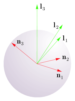
Figure 3: Duality of basic sets $\{{\bf n}_{k}\}_{k=1}^{3}$ and $\{{\bf l}_{k}\}_{k=1}^{3}$. Any qubit state is identified with a six-dimensional probability vector $\boldsymbol{\cal P}$, which is composed of three spin-$1/2$ portraits ${\bf w}_{1/2}^{(1/2)}({\bf n}_{1})$, ${\bf w}_{1/2}^{(1/2)}({\bf n}_{2})$, and ${\bf w}_{1/2}^{(1/2)}({\bf n}_{3})$ given by vectors ${\bf n}_{1}$, ${\bf n}_{2}$, and ${\bf n}_{3}$, respectively. Vectors $\{{\bf l}_{k}\}_{k=1}^{3}$ form a dual vector basis that determines the inverse map (76) of the vector $\boldsymbol{\cal P}$ onto a qubit density operator. The map is bijective whenever vectors ${\bf n}_{1}$, ${\bf n}_{2}$, and ${\bf n}_{3}$ are noncoplanar.

Thus, the vectors $\{{\bf l}_{k}\}_{k=1}^{3}$ form a dual basis with respect to the directions $\{{\bf n}_{k^{\prime}}\}_{k^{\prime}=1}^{3}$, i.e., $({\bf l}_{k}\cdot{\bf n}_{k^{\prime}})=\delta_{kk^{\prime}}$. This dual basis can be used to construct dual symbols of operators [41, 42]. Note that vectors $\{{\bf l}_{k}\}_{k=1}^{3}$ are no longer normalized. Figure 3 illustrates the duality of basic sets $\{{\bf n}_{k}\}_{k=1}^{3}$ and $\{{\bf l}_{k}\}_{k=1}^{3}$ and, consequently, the duality of mappings $\hat{\rho}\rightarrow\boldsymbol{\cal P}$ and $\boldsymbol{\cal P}\rightarrow\hat{\rho}$.

Using the special properties of Pauli matrices, one can easily calculate the star-product kernel (7). The result is

$$K^{(1/2)}(m_{3},{\bf n}_{k_{3}},m_{2},{\bf n}_{k_{2}},m_{1},{\bf n}_{k_{1}}) = 3\Big{\{}\frac{1}{4}\delta_{k_{3},1}\delta_{k_{2},1}+\delta_{k_{3},1}m_{2}m_{1}({\bf l}_{k_{2}}\cdot{\bf n}_{k_{1}})+\delta_{k_{2},1}m_{3}m_{1}({\bf l}_{k_{3}}\cdot{\bf n}_{k_{1}})$$ (78)

$$\quad+m_{3}m_{2}({\bf l}_{k_{3}}\cdot{\bf l}_{k_{2}})+2im_{3}m_{2}m_{1}([{\bf l}_{k_{3}}\times{\bf l}_{k_{2}}]\cdot{\bf n}_{k_{1}})\Big{\}}.$$

The intertwining kernels (73) and (75) take the following form:

$$K_{w\rightarrow{\cal P}}^{(1/2)}(m,{\bf n}_{k},m^{\prime},{\bf n}^{\prime})=\frac{1}{6}+2m^{\prime}m({\bf n}^{\prime}\cdot{\bf n}_{k}),\qquad K_{{\cal P}\rightarrow w}^{(1/2)}(m,{\bf n},m^{\prime},k^{\prime})=3\left\{\frac{1}{2}\delta_{k^{\prime},1}+2m^{\prime}m({\bf l}_{k^{\prime}}\cdot{\bf n})\right\}.$$

As far as qutrits are concerned, any quantum state can be associated either with the fifteen-dimensional probability vector (45) parameterized by five $SU(2)$ rotations or the twelve-dimensional probability vector (54) written in terms of four $SU(3)$ rotations in the Hilbert space. The former case implies that the vector $\boldsymbol{\cal P}$ comprises five qutrit portraits, each defined by the direction ${\bf n}_{k}$, $k=1,\dots,5$. The density operator is uniquely determined whenever these directions satisfy the condition (53). The latter case of $SU(3)$ rotations implies the limitation (58) on unitary matrices $u_{k^{\prime}}$, $k^{\prime}=1,\dots,4$.

The explicit formula of the density operator in terms of experimentally attainable probabilities ${\cal P}_{\rm eq}(m,{\bf n}_{k})$ reads

$$\hat{\rho}=\frac{1}{3}\left[{\cal P}_{\rm eq}(+1,{\bf n}_{1})+{\cal P}_{\rm eq}(0,{\bf n}_{1})+{\cal P}_{\rm eq}(-1,{\bf n}_{1})\right]\hat{I}+\frac{1}{2}\sum_{k=1}^{3}\left[{\cal P}_{\rm eq}(+1,{\bf n}_{k})-{\cal P}_{\rm eq}(-1,{\bf n}_{k})\right](\hat{\bf J}\cdot{\bf l}_{k})$$

$$+\frac{1}{6}\left(\begin{array}[]{c}{\cal P}_{\rm eq}(+1,{\bf n}_{1})-2{\cal P}_{\rm eq}(0,{\bf n}_{1})+{\cal P}_{\rm eq}(-1,{\bf n}_{1})\\ {\cal P}_{\rm eq}(+1,{\bf n}_{2})-2{\cal P}_{\rm eq}(0,{\bf n}_{2})+{\cal P}_{\rm eq}(-1,{\bf n}_{2})\\ {\cal P}_{\rm eq}(+1,{\bf n}_{3})-2{\cal P}_{\rm eq}(0,{\bf n}_{3})+{\cal P}_{\rm eq}(-1,{\bf n}_{3})\\ {\cal P}_{\rm eq}(+1,{\bf n}_{4})-2{\cal P}_{\rm eq}(0,{\bf n}_{4})+{\cal P}_{\rm eq}(-1,{\bf n}_{4})\\ {\cal P}_{\rm eq}(+1,{\bf n}_{5})-2{\cal P}_{\rm eq}(0,{\bf n}_{5})+{\cal P}_{\rm eq}(-1,{\bf n}_{5})\\ \end{array}\right)^{T}$$ (85)

$$\times\left\|\begin{array}[]{ccccc}1&\frac{3({\bf n}_{1}\cdot{\bf n}_{2})^{2}-1}{2}&\frac{3({\bf n}_{1}\cdot{\bf n}_{3})^{2}-1}{2}&\frac{3({\bf n}_{1}\cdot{\bf n}_{4})^{2}-1}{2}&\frac{3({\bf n}_{1}\cdot{\bf n}_{5})^{2}-1}{2}\\ \frac{3({\bf n}_{2}\cdot{\bf n}_{1})^{2}-1}{2}&1&\frac{3({\bf n}_{2}\cdot{\bf n}_{3})^{2}-1}{2}&\frac{3({\bf n}_{2}\cdot{\bf n}_{4})^{2}-1}{2}&\frac{3({\bf n}_{2}\cdot{\bf n}_{5})^{2}-1}{2}\\ \frac{3({\bf n}_{3}\cdot{\bf n}_{1})^{2}-1}{2}&\frac{3({\bf n}_{3}\cdot{\bf n}_{2})^{2}-1}{2}&1&\frac{3({\bf n}_{3}\cdot{\bf n}_{4})^{2}-1}{2}&\frac{3({\bf n}_{3}\cdot{\bf n}_{5})^{2}-1}{2}\\ \frac{3({\bf n}_{4}\cdot{\bf n}_{1})^{2}-1}{2}&\frac{3({\bf n}_{4}\cdot{\bf n}_{2})^{2}-1}{2}&\frac{3({\bf n}_{4}\cdot{\bf n}_{3})^{2}-1}{2}&1&\frac{3({\bf n}_{4}\cdot{\bf n}_{5})^{2}-1}{2}\\ \frac{3({\bf n}_{5}\cdot{\bf n}_{1})^{2}-1}{2}&\frac{3({\bf n}_{5}\cdot{\bf n}_{2})^{2}-1}{2}&\frac{3({\bf n}_{5}\cdot{\bf n}_{3})^{2}-1}{2}&\frac{3({\bf n}_{5}\cdot{\bf n}_{4})^{2}-1}{2}&1\\ \end{array}\right\|^{-1}\left(\begin{array}[]{c}3(\hat{\bf J}\cdot{\bf n}_{1})^{2}-2\hat{I}\\ 3(\hat{\bf J}\cdot{\bf n}_{2})^{2}-2\hat{I}\\ 3(\hat{\bf J}\cdot{\bf n}_{3})^{2}-2\hat{I}\\ 3(\hat{\bf J}\cdot{\bf n}_{4})^{2}-2\hat{I}\\ 3(\hat{\bf J}\cdot{\bf n}_{5})^{2}-2\hat{I}\\ \end{array}\right).$$ (96)

A similar reconstruction of qutrit states is proposed in [44]. Higher spins ($S=4$) are reconstructed in [45]. The advantage of the proposed inverse mapping (62) is that it can be applied to a system with an arbitrary spin $j$ and provides the explicit solution in an operator form.

9 Quantum States on 2j(4j+3)-Simplex

We already know that any quantum state can be associated with the probability-distribution vector $\boldsymbol{\cal P}$. If $SU(2)$ rotations underlie the construction of the vector $\boldsymbol{\cal P}$, this vector comprises $(2j+1)(4j+1)$ components ${\cal P}(m,{\bf n}_{k})$. Consequently, it is represented by a point on the simplex with dimension $(2j+1)(4j+1)-1=2j(4j+3)$. Conversely, not all points on the $2j(4j+3)$ simplex can be associated with quantum states. Indeed, the condition $\hat{\rho}\geq 0$ is to be satisfied. Let us reformulate this requirement in terms of components ${\cal P}(m,{\bf n}_{k})$.

In view of the inverse map (62), we readily obtain the following condition:

$$\sum_{L=0}^{2j}\sum_{k=1}^{2L+1}\sum_{m=-j}^{j}{\cal P}_{\rm eq}(m,{\bf n}_{k})f_{L}^{(j)}(m)\sum_{k^{\prime}=1}^{2L+1}\|\mathscr{M}^{-1}(L)\|_{kk^{\prime}}\hat{S}_{L}^{(j)}({\bf n}_{k^{\prime}})\geq 0.$$ (98)

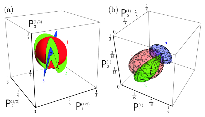
Figure 4: Convex subset of quantum states on the $2j(4j+3)$-simplex. In the case of qubits, ${\cal P}_{\rm eq}(+1/2,{\bf n}_{1})=\mathsf{P}_{1}^{(1/2)}$, ${\cal P}_{\rm eq}(-1/2,{\bf n}_{1})=1/3-\mathsf{P}_{1}^{(1/2)}$, ${\cal P}_{\rm eq}(+1/2,{\bf n}_{2})=\mathsf{P}_{2}^{(1/2)}$, ${\cal P}_{\rm eq}(-1/2,{\bf n}_{2})=1/3-\mathsf{P}_{2}^{(1/2)}$, ${\cal P}_{\rm eq}(+1/2,{\bf n}_{3})=\mathsf{P}_{3}^{(1/2)}$, and ${\cal P}_{\rm eq}(-1/2,{\bf n}_{3})=1/3-\mathsf{P}_{3}^{(1/2)}$ (a). So any point on the $\boldsymbol{\cal P}$-simplex is uniquely determined by a point $\left(\mathsf{P}_{1}^{(1/2)},\mathsf{P}_{2}^{(1/2)},\mathsf{P}_{3}^{(1/2)}\right)$ inside a cube $\{0\leq\mathsf{P}_{k}^{(1/2)}\leq 1/3\}_{k=1}^{3}$, where quantum subsets are shown for $({\bf n}_{1}\cdot[{\bf n}_{2}\times{\bf n}_{3}])=1$ (1), $0.44$ (2), and $0.02$ (3). In the case of qutrits, simplex is fourteen-dimensional (b), where we fix five directions in such a way that $({\bf n}_{1}\cdot{\bf n}_{2})=({\bf n}_{2}\cdot{\bf n}_{3})=({\bf n}_{3}\cdot{\bf n}_{1})=({\bf n}_{1}\cdot{\bf n}_{4})=({\bf n}_{2}\cdot{\bf n}_{4})=({\bf n}_{1}\cdot{\bf n}_{5})=({\bf n}_{3}\cdot{\bf n}_{5})=1/\sqrt{3}$. Denote $\mathsf{P}_{k}^{(1)}={\cal P}_{\rm eq}(+1,{\bf n}_{k})$, $k=1,2,3$, then the cut set ${\cal P}_{\rm eq}(+1,{\bf n}_{4})={\cal P}_{\rm eq}(+1,{\bf n}_{5})=1/15$, and ${\cal P}_{\rm eq}(-1,{\bf n}_{k^{\prime}})=1/15$, ${k^{\prime}}=1,\dots,5$ corresponds to 1, the cut set ${\cal P}_{\rm eq}(+1,{\bf n}_{4})={\cal P}_{\rm eq}(+1,{\bf n}_{5})=1/15$, and ${\cal P}_{\rm eq}(-1,{\bf n}_{k^{\prime}})=1/15$, ${k^{\prime}}=1,\dots,5$ corresponds to 2, and the cut set ${\cal P}_{\rm eq}(+1,{\bf n}_{4})={\cal P}_{\rm eq}(+1,{\bf n}_{5})=1/20$, and ${\cal P}_{\rm eq}(-1,{\bf n}_{k^{\prime}})=1/20$, ${k^{\prime}}=1,\dots,5$ corresponds to 3.

This implies that the matrix of the operator (98) in the basis of states $|jm\rangle$ is nonnegative. Nonnegativity of such a matrix is easily checked by Sylvester’s criterion [43]; namely, it is necessary and sufficient that all principal minors of matrix (98) are nonnegative.

Let us consider the case of qubits ($j=1/2$) in detail.

From explicit formula (76), it is readily seen that vector $\boldsymbol{\cal P}_{\rm eq}$ determines a quantum state iff

$$\left\{\begin{array}[]{c}\frac{1}{2}[{\cal P}_{\rm eq}(+1/2,{\bf n}_{1})+{\cal P}_{\rm eq}(-1/2,{\bf n}_{1})]+\sum_{k=1}^{3}[{\cal P}_{\rm eq}(+1/2,{\bf n}_{k})-{\cal P}_{\rm eq}(-1/2,{\bf n}_{k})]\big{(}{\bf l}_{k}\cdot(0,0,1)\big{)}\geq 0,\\ \frac{1}{4}[{\cal P}_{\rm eq}(+1/2,{\bf n}_{1})+{\cal P}_{\rm eq}(-1/2,{\bf n}_{1})]^{2}-\left(\sum_{k=1}^{3}[{\cal P}_{\rm eq}(+1/2,{\bf n}_{k})-{\cal P}_{\rm eq}(-1/2,{\bf n}_{k})]{\bf l}_{k}\right)^{2}\geq 0,\\ \frac{1}{2}[{\cal P}_{\rm eq}(+1/2,{\bf n}_{1})+{\cal P}_{\rm eq}(-1/2,{\bf n}_{1})]-\sum_{k=1}^{3}[{\cal P}_{\rm eq}(+1/2,{\bf n}_{k})-{\cal P}_{\rm eq}(-1/2,{\bf n}_{k})]\big{(}{\bf l}_{k}\cdot(0,0,1)\big{)}\geq 0.\\ \end{array}\right.$$ (99)

Taking into account the relation ${\cal P}_{\rm eq}(+1/2,{\bf n}_{k})+{\cal P}_{\rm eq}(-1/2,{\bf n}_{k})=1/3$, $k=1,2,3$, the obtained system of inequalities can be easily depicted (Fig. 4a). Indeed, using such a constrain on the probabilities, the five-simplex for six-component vector $\boldsymbol{\cal P}$ is identified with the interior of the cube $0\leq{\cal P}_{\rm eq}(+1/2,{\bf n}_{k})\leq 1/3$, $k=1,2,3$. Quantum states are those points on the simplex that satisfy the conditions (99). In particular, if $\{{\bf n}_{k}\}_{k=1}^{3}$ form an orthonormal basis in $\mathbb{R}^{3}$, the quantum states are associated with the ball

$$\left({\cal P}_{\rm eq}(+1/2,{\bf n}_{1})-\frac{1}{6}\right)^{2}+\left({\cal P}_{\rm eq}(+1/2,{\bf n}_{2})-\frac{1}{6}\right)^{2}+\left({\cal P}_{\rm eq}(+1/2,{\bf n}_{3})-\frac{1}{6}\right)^{2}\leq\frac{1}{144}.$$ (100)

The general case of arbitrary directions $\{{\bf n}_{k}\}_{k=1}^{3}$ is shown in Fig. 4a.

In the case of qutrits ($j=1$), we restrict ourselves to a numerical solution of the system of seven inequalities analogous to (99). It is worth noting that the quantum domain on the fourteen-simplex is given by algebraic inequalities — three inequalities of the first order, three inequalities of the second order, and one inequality of the third order. Different cut sets of this simplex by hyperplanes ${\cal P}_{\rm eq}(-1,{\bf n}_{4})={\cal P}_{\rm eq}(-1,{\bf n}_{5})={\rm const}$ and ${\cal P}_{\rm eq}(0,{\bf n}_{k})={\rm const}$, $k=1,\dots,5$ are illustrated in Fig. 4b. The cut set of qutrit states is a third-degree body of the vector elements ${\cal P}_{\rm eq}(+1,{\bf n}_{1})$, ${\cal P}_{\rm eq}(+1,{\bf n}_{2})$, and ${\cal P}_{\rm eq}(+1,{\bf n}_{3})$, with the cut set being located between three planes and three second-degree surfaces.

10 Conclusions

To conclude, a bijective map of qudit-$j$ states onto single probability vectors $\boldsymbol{\cal P}$ has been developed. In fact, any quantum state is associated with such a probability vector. Quantum states form a convex subset on a simplex of possible probability vectors $\boldsymbol{\cal P}$, with the boundary of quantum states being the $(2j+1)$-degree body of vector elements ${\cal P}(m,u)$. Examples of quantum subsets are presented for qubits ($j=1/2$) and qutrits ($j=1$). Components ${\cal P}(m,u)$ are fair probabilities, have a clear physical meaning, and can be relatively easily measured experimentally.

To be precise, ${\cal P}(m,u_{k})$ is a joint probability distribution function of two discrete variables – spin projection $m$ and unitary rotation $u_{k}$ from a finite set of rotations $\{u_{k}\}_{k=1}^{N_{u}}$. The number of rotations $N_{u}$ is shown to depend on the type of rotations used. Namely, $N_{u}=2j+2$ if all unitary matrices $u_{k}$ are elements of the group $SU(N)$ with $N=2j+1$, and $N_{u}=4j+1$ if $u_{k}\in SU(2)$ for all $k$. The latter case is considered in detail. The dequantizer operator $\hat{\cal U}^{(j)}(m,{\bf n}_{k})$ specifying the direct map $\hat{\rho}\rightarrow\boldsymbol{\cal P}_{\rm eq}$ and the quantizer operator $\hat{\cal D}^{(j)}(m,{\bf n}_{k})$ specifying the inverse map $\boldsymbol{\cal P}_{\rm eq}\rightarrow\hat{\rho}$ are presented in the explicit form for an arbitrary choice of directions $\{{\bf n}_{k}\}_{k=1}^{4j+1}$. The kernel of the corresponding star-product quantization scheme as well as intertwining kernels relating ${\cal P}$-representation and $w$-tomographic representation are found.

A subsidiary problem of the optimum choice of directions $\{{\bf n}_{k}\}_{k=1}^{4j+1}$ is discussed and partially solved for the low spin states, with the optimality implying the minimum relative error $\|\delta\hat{\rho}\|_{2}$ if errors $\delta\boldsymbol{\cal P}$ in the measured probability vector $\boldsymbol{\cal P}$ are presented.

Last, but not least, different mappings of density operators onto the probability vectors are unified within the concept of the inverse spin-$s$ portrait method. The difference between mappings reduces to a particular choice of spin-$s$ portraits implicitly used in these transforms; namely, [12, 20] rely on spin-$1/2$ portraits, whereas [7, 44] extensively employ spin-$j$ portraits.

References

- [1] L. D. Landau, Ztschr. Phys., 45, 430 (1927).
- [2] J. von Neumann, Göttingen. Nachr., 245 (1927).
- [3] U. Fano, Rev. Mod. Phys., 29, 74 (1957).
- [4] A. Vourdas, J. Phys. A: Math. Gen., bf 39, R65 (2006).
- [5] V. V. Dodonov and V. I. Man’ko, Phys. Lett. A, 229, 335 (1997).
- [6] V. I. Man’ko and O. V. Man’ko, J. Exp. Theor. Phys., 85, 430 (1997).
- [7] R. G. Newton and B. Young, Ann. Phys., 49, 393 (1968).
- [8] S. Weigert, Phys. Rev. A, 45, 7688 (1992).
- [9] J.-P. Amiet and S. Weigert, J. Phys. A: Math. Gen., 31, L543 (1998).
- [10] J.-P. Amiet and S. Weigert, J. Phys. A: Math. Gen., 32, 2777 (1999).
- [11] J.-P. Amiet and S. Weigert, J. Opt. B: Quantum Semiclass. Opt., 1, L5 (1999).
- [12] J.-P. Amiet and S. Weigert, J. Phys. A: Math. Gen., 32, L269 (1999).
- [13] S. Weigert, Phys. Rev. Lett., 84, 802 (2000).
- [14] J.-P. Amiet and S. Weigert, J. Opt. B: Quantum Semiclass. Opt., 2, 118 (2000).
- [15] S. Heiss and S. Weigert, Phys. Rev. A, 63, 012105 (2000).
- [16] C. A. Fuchs and M. Sasaki, Quantum Inform. Comput., 3, 277 (2003).
- [17] C. A. Fuchs, Quantum Inform. Comput., 4, 467 (2004).
- [18] D. M. Appleby, H. B. Dang, and C. A. Fuchs, “Physical significance of symmetric informationally-complete sets of quantum states,” Los Alamos Arxiv, quant-ph/0707.2071 (2007).
- [19] C. A. Fuchs and R. Schack, Found. Phys., DOI: 10.1007/s10701-009-9404-8 (2010).
- [20] D. M. Appleby, Å. Ericsson and C. A. Fuchs, “Properties of -bit State Spaces,” Los Alamos Arxiv, quant-ph/0910.2750 (2009).
- [21] D. M. Appleby, S. T. Flammia, and C. A. Fuchs, “The Lie algebraic significance of symmetric informationally complete measurements,” Los Alamos Arxiv, quant-ph/1001.0004 (2010).
- [22] V. I. Man’ko, G. Marmo, E. C. G. Sudarshan, and F. Zaccaria, Phys. Lett. A, 327, 353 (2004).
- [23] V. A. Andreev and V. I. Man’ko, J. Exp. Theor. Phys., 87, 239 (1998).
- [24] O. V. Man’ko, V. I. Man’ko, and S. S. Safonov, Theor. Math. Phys., 115, 185 (1998).
- [25] V. A. Andreev, O. V. Man’ko, V. I. Man’ko, and S. S. Safonov, J. Russ. Laser Res., 19, 340 (1998).
- [26] O. V. Man’ko and V. I. Man’ko, J. Russ. Laser Res., 18, 407 (1997).
- [27] O. Castaños, R. López-Peña, M. A. Man’ko, and V. I. Man’ko, J. Phys. A: Math. Gen., 36, 4677 (2003).
- [28] G. M. D’Ariano, L. Maccone, and M. Paini, J. Opt. B: Quantum Semicl. Opt., 5, 77 (2003).
- [29] S. N. Filippov and V. I. Man’ko, J. Russ. Laser Res., 30, 82 (2009).
- [30] A. F. Nikiforov, S. K. Suslov, and V. B. Uvarov, Classical Orthogonal Polynomials of a Discrete Variable, Springer Verlag, Berlin, Heidelberg, New York (1991).
- [31] A. F. Nikiforov and V. B. Uvarov, Special Functions of Mathematical Physics, Birkhauser Verlag, Basel, Boston (1988).
- [32] V. N. Chernega and V. I. Man’ko, J. Russ. Laser Res., 28, 2 (2007).
- [33] C. Lupo, V. I. Man’ko, and G. Marmo, J. Phys. A: Math. Theor., 40, 13091 (2007).
- [34] S. N. Filippov and V. I. Man’ko, J. Russ. Laser Res., 30, 55 (2009).
- [35] G. H. Golub and C. F. Van Loan, Matrix Computations, The Johns Hopkins University Press, Baltimore and London (1996).
- [36] A. Ibort, V. I. Man’ko, G. Marmo, A. Simoni, and F. Ventriglia, Phys. Scr., 79, 065013 (2009).
- [37] F. R. Gantmacher, The Theory of Matrices, AMS Chelsea Publishing, Providence, RI (1998).
- [38] O. V. Man’ko, V. I. Man’ko, and G. Marmo, Phys. Scr., 62, 446 (2000).
- [39] O. V. Man’ko, V. I. Man’ko, and G. Marmo, J. Phys. A: Math. Gen., 35, 699 (2002).
- [40] O. V. Man’ko, J. Russ. Laser Res., 28, 483 (2007).
- [41] V. I. Man’ko, G. Marmo, and P. Vitale, Phys. Lett. A, 334, 1 (2005).
- [42] O. V. Man’ko, V. I. Man’ko, G. Marmo, and P. Vitale, Phys. Lett. A, 360, 522 (2007).
- [43] C. D. Meyer, Matrix Analysis and Applied Linear Algebra, SIAM, Philadelphia, PA (2000).
- [44] H. F. Hofmann and S. Takeuchi, Phys. Rev. A, 69, 042108 (2004).
- [45] G. Klose, G. Smith, and P. S. Jessen, Phys. Rev. A, 86, 4721 (2001).