Quantum Limits on Parameter Estimation

Abstract

We present a new proof of the quantum Cramer-Rao bound for precision parameter estimation key-1 ; key-2 ; key-3 and extend it to a more general class of measurement procedures. We analyze a generalized framework for parameter estimation that covers most experimentally accessible situations, where multiple rounds of measurements, auxiliary systems or external control of the evolution are available. The proof presented demonstrates the equivalence of these more general metrology procedures to the simplest optimal strategy for which the bound is proven: a single measurement of a two-level system interacting with a time-independent Hamiltonian.

I Introduction

High sensitivity parameter estimation is an active area of research in quantum physics. There is growing effort both theoretically and experimentally to use quantum properties of matter to improve the precision with which a given parameter may be estimated. These ideas have been used in several problems of practical interest; namely, clock synchronization key-4 ; key-5 ; key-6 ; key-7 ; key-8 , reference frame alignment key-9 ; key-10 , phase estimation key-11 ; key-12 ; key-13 , frequency measurements key-14 ; key-15 ; key-16 ; key-17 , position measurements key-18 ; key-19 and magnetometry key-20 ; key-21 . The simplest procedure for parameter estimation uses a probe which is coupled to the external field ($b$) to be measured by a Hamiltonian $b\,H$. The probe is prepared in a well-known initial state and then interacts with the field for a time $\tau$ before the measurement of a suitable observable $\mathcal{O}$. The process is then repeated for a large number of times ($N$) to improve statistics.

Many different strategies have been proposed to improve the sensitivity limit of the simple parameter estimation procedure Giovannetti06 . For example, the probe can be a composite system Wineland92 or be augmented by ancillary systems used for multiple quantum non-demolition (QND) measurements key-22 . The external field Hamiltonian can be manipulated by additional field-independent and controllable Hamiltonians to obtain an effective Hamiltonian $b\,\bar{H}$ key-14 ; key-15 ; key-16 ; key-17 ; key-20 ; key-21 . During the evolution time $\tau$ many positive operator valued measurements (POVMs) can be performed and the results of the measurements used in a feedback loop key-23 ; key-24 . The only constraint on the metrology procedure is that a single measurement time is limited to $\tau$. This assumption is physically motivated as any measurement process suffers from decoherence that limits the sensing time.

The quantum Cramer-Rao bound gives a bound on the achievable sensitivity key-1 ; key-2 ; key-3 . For any measurement scheme, if the largest and smallest eigenvalues of $H$ are $\Lambda$ and $\lambda$, respectively, the optimum possible sensitivity is bounded by:

$$\delta b\geq\frac{1}{\tau\sqrt{N}\left(\Lambda-\lambda\right)},$$ (1)

where $N$ is the number of measurement runs and we set $\hbar=1$. This is very similar to the Heisenberg limit for precision measurements with entangled states where in the Heisenberg limit $\Lambda-\lambda$ is related to the number of entangled spins used for the quantum measurement key-26 (27).

In this paper we present a new rigorous proof of this theorem. Our approach is to reduce general parameter estimation problems often studied in the literature (involving e.g. larger systems, mixed states or POVMs) to the case of a two-level system. Furthermore we extend the bound validity showing that multiple rounds of POVMs and feedback cannot improve this limit.

We first prove in Section II the sensitivity bound for a single POVM measurement on an isolated two-level system in a pure state. The proof relies on the classical Fisher Information (reviewed in the Appendix), which provides a lower bound on the uncertainty of parameter estimation via multiple measurements in terms of the probabilities of various measurement outcomes. We then show in Section III that for the purposes of precision measurement a general $N$-level system prepared in a pure state is equivalent to a two-level system. Specifically, we will demonstrate an explicit reduction of the $N$-level system to one of its two dimensional subspaces; then extend these results to the case where a control Hamiltonian is added to the field dependent Hamiltonian ($H=b\,H+H_{0}$ ) by going to an appropriate interaction picture. By using “convexity” properties of Fisher Information and Cauchy-Schwartz inequalities, we also prove in Section IV the bound for mixed states.

In section V we further prove that these results are still valid when feedback during the measurement and classical communication between different measurement rounds are available, situations where the Cramer-Rao bound has not been proved before.

Finally, in Section VI, we give an example of an experimentally accessible system where the proven bound can be satisfied, before drawing our conclusions in Section VII.

II Bound for a Single Two-Level System Prepared in a Pure State

Lemma 1 – Consider parameter estimation using a single two level system. Suppose that the system interacts with the Hamiltonian $b\cdot H$ (with largest and smallest eigenvalues $\Lambda$ and $\lambda$ respectively) for a time $\tau$. The system is initialized in the state $\left|\Psi_{in}\right\rangle$ and at the end of the sensing sequence an operator $\mathcal{O}$ is measured . The procedure is repeated $N$ times. Then, the minimum uncertainty of $b$ is given by:

$${\displaystyle\inf_{\left|\Psi_{in}\right\rangle,\mathcal{O}}\delta b=\frac{1}{\tau\sqrt{N}\left(\Lambda-\lambda\right)},}$$ (2)

where the infimum is taken over all initial states $\left|\Psi_{in}\right\rangle$ and observables $\mathcal{O}$.

Proof – Given an operator $\mathcal{O}$, the precision with which $b$ can be determined is given by:

$$\delta b=\frac{\langle\Psi_{fin}|\Delta\mathcal{O}|\Psi_{fin}\rangle}{\sqrt{N}|\partial\langle\Psi_{fin}|\mathcal{O}|\Psi_{fin}\rangle/\partial b|}\approx\frac{\left\langle\Psi_{in}\right|\Delta\mathcal{O}\left|\Psi_{in}\right\rangle}{\tau\sqrt{N}\left|\left\langle\Psi_{in}\right|\left[H,\mathcal{O}\right]\left|\Psi_{in}\right\rangle\right|},$$ (3)

where $|\Psi_{fin}\rangle=e^{-ib\,Ht}\left|\Psi_{in}\right\rangle$ and the second line is obtained by first order perturbation theory.

First we show that the limit given by Eq. (2) above can be attained. Explicitly if we choose $\mathcal{O}=\left|\Lambda\right\rangle\left\langle\lambda\right|+\left|\lambda\right\rangle\left\langle\Lambda\right|$ and $\left|\Psi_{in}\right\rangle=\frac{1}{\sqrt{2}}\left(\left|\Lambda\right\rangle+i\left|\lambda\right\rangle\right)$, we obtain $\frac{\left|\left\langle\Psi_{in}\right|\left[H,\mathcal{O}\right]\left|\Psi_{in}\right\rangle\right|}{\left\langle\Delta\mathcal{O}\right\rangle}=\Lambda-\lambda$.

To prove that this is the optimal bound we consider a general initial state and measurement Hamiltonian. First we observe that Eq. (2) is invariant under the substitutions $H\rightarrow\kappa H+\mu\leavevmode\hbox{\small 1\normalsize\kern-3.30002pt1}$ and $\mathcal{O}\rightarrow\chi\mathcal{O}+\nu\leavevmode\hbox{\small 1\normalsize\kern-3.30002pt1}$. As a result we can take $H=\overrightarrow{h}\cdot\overrightarrow{\sigma}$ and $\mathcal{O}=\overrightarrow{o}\cdot\overrightarrow{\sigma}$ (with $\left\|\overrightarrow{h}\right\|,\left\|\overrightarrow{o}\right\|=1$). Because of rotational invariance of Eq. (2), without loss of generality we can assume that $H=\frac{\sigma_{z}}{2}$ and $\mathcal{O}=\cos{\alpha}\,\sigma_{z}+\sin{\alpha}\,\sigma_{x}$, with initial state $|\Psi_{in}\rangle=\cos{(\vartheta/2)}|0\rangle+e^{i\varphi/2}\sin{(\vartheta/2)}|1\rangle$. Then $\langle\mathcal{O}\rangle=\cos{\alpha}\cos{\vartheta}+\sin{\alpha}\sin{\vartheta}\cos{\left(bt-\varphi/2\right)}$, and since $\mathcal{O}^{2}=\leavevmode\hbox{\small 1\normalsize\kern-3.30002pt1}$, the uncertainty in the external field is given by

$$\delta b=\frac{\sqrt{1-\left[\cos{\alpha}\cos\theta+\sin\alpha\sin{\vartheta}\cos{\left(bt-\frac{\phi}{2}\right)}\right]^{2}}}{t\sin{\alpha}\sin{\vartheta}\sin\left(bt-\frac{\varphi}{2}\right)}.$$

Taking the derivative with respect to $\alpha$ and $\vartheta$, we find that the maximum is obtained $\forall\varphi$ for $\alpha=\pm\pi/2$ and $\vartheta=\pm\pi/2$ and it is equal to $\delta b=\frac{1}{\tau\sqrt{N}}$ (which matches Eq. (2) given that the spread of eigenvalues of $\frac{\sigma_{z}}{2}$ is one).$\hfill\Box\vspace{8pt}$

Lemma 2 – Consider parameter estimation using a single two level system. Suppose the system interacts with the external field via an effective Hamiltonian $b\,H$. The largest and smallest eigenvalues of $H$ are $\Lambda$ and $\lambda$ respectively. The system is initialized in a state $\left|\Psi_{in}\right\rangle$ and after a time $\tau$ a generalized measurement described by a set of POVMs $\left\{E_{\alpha}\right\}$ is performed. If this procedure is repeated $N$ times, the minimum uncertainty of $b$ is:

$$\delta b_{min}\equiv{\displaystyle\inf_{\left|\Psi_{in}\right\rangle,\left\{E_{\alpha}\right\}}\delta b=\frac{1}{\tau\sqrt{N}\left(\Lambda-\lambda\right)},}$$ (4)

where the infimum is taken over all initial states $\left|\Psi_{in}\right\rangle$ and POVMs $\left\{E_{\alpha}\right\}$ .

Proof – Let $\left\{E_{1},\,E_{2},...E_{K}\right\}$ be any POVM, and $\left|\Psi_{in}\right\rangle$ any given initial state. To first order in $b$, the probability of the measurement outcome being $E_{\alpha}$ is given by $P\left(E_{\alpha}\right)=\left\langle\Psi_{fin}\right|E_{\alpha}\left|\Psi_{fin}\right\rangle\approx\left\langle\Psi_{in}\right|E_{\alpha}\left|\Psi_{in}\right\rangle+ib\tau\left\langle\Psi_{in}\right|\left[H,E_{\alpha}\right]\left|\Psi_{in}\right\rangle\equiv P_{0}\left(E_{\alpha}\right)+b\delta P\left(E_{\alpha}\right)$. Then, by Lemma 3 in the Appendix (classical Fisher information), the uncertainty in the external field is:

$$\delta b_{min}^{2}=\left({N\sum\frac{\left(i\tau\left\langle\Psi_{in}\right|\left[H,E_{\alpha}\right]\left|\Psi_{in}\right\rangle\right)^{2}}{\left\langle\Psi_{in}\right|E_{\alpha}\left|\Psi_{in}\right\rangle}}\right)^{-1}$$ (5)

Furthermore, according to Sublemma 1 (see Eq. 19 in the Appendix) the same sensitivity may be obtained by measuring the operator $\mathcal{O}\equiv\sum_{\alpha}\frac{E_{\alpha}}{P_{0}\left(E_{\alpha}\right)}$. We have thus reduced the problem to the case where we measure a single operator and we may apply the results of Lemma 1 to obtain the bound (4). $\hfill\Box\vspace{8pt}$

III Cramer-Rao Bound For Higher Dimensional Systems

We will now reduce parameter estimation with general pure states to the two dimensional case studied in Lemma 1.

Proposition 1 – Consider parameter estimation with an arbitrary probe in an $n$-dimensional Hilbert space. Suppose that the system interacts with the external field via the Hamiltonian $b\,H$ (with largest and smallest eigenvalues $\Lambda$ and $\lambda$ respectively) for a time $\tau$. The system is initialized in the state $\left|\Psi_{in}\right\rangle$ and at the end of the sensing sequence a POVM measurement with operators $\left\{E_{\alpha}\right\}$ is performed. The procedure is repeated $N$ times. Then the minimum uncertainty $\delta b_{min}$ is given by Eq. (1).

Proof – We reformulate the $n$-dimensional problem in terms of the two-dimensional case we just proved.

For any initial state $\left|\Psi_{in}\right\rangle$ we define $\left|\Omega_{in}\right\rangle\equiv H\left|\Psi_{in}\right\rangle$. We can reduce the measurement procedure to a measurement on the subspace $V_{S}$ spanned by $\left\{\left|\Psi_{in}\right\rangle,\,\left|\Omega_{in}\right\rangle\right\}$ since

$$\begin{array}[]{ll}\delta b_{min}^{2}&=\left(N\sum\frac{\left(ib\tau\left\{\left\langle\Omega_{in}\right|E_{\alpha}\left|\Psi_{in}\right\rangle-\left\langle\Psi_{in}\right|E_{\alpha}\left|\Omega_{in}\right\rangle\right\}\right)^{2}}{\left\langle\Psi_{in}\right|E_{\alpha}\left|\Psi_{in}\right\rangle}\right)^{-1}\\ &=\left({N\sum\frac{\left(ib\tau\left\{\left\langle\Omega_{in}\right|\Pi E_{\alpha}\Pi\left|\Psi_{in}\right\rangle-\left\langle\Psi_{in}\right|\Pi E_{\alpha}\Pi\left|\Omega_{in}\right\rangle\right\}\right)^{2}}{\left\langle\Psi_{in}\right|\Pi E_{\alpha}\Pi\left|\Psi_{in}\right\rangle}}\right)^{-1},\end{array}$$ (6)

where $\Pi$ is the projector onto the space spanned by $\left|\Omega_{in}\right\rangle$ and $\left|\Psi_{in}\right\rangle$. When restricted to the two dimensional subspace spanned by $\{\left|\Psi_{in}\right\rangle,\ \left|\Omega_{in}\right\rangle\}$ the set of operators $\left\{\Pi E_{\alpha}\Pi\right\}$ still forms a POVM, since all the operators are positive definite $\left\langle\Psi\right|\Pi E_{\alpha}\Pi\left|\Psi\right\rangle\geq 0$ and $\sum\Pi E_{\alpha}\Pi=\leavevmode\hbox{\small 1\normalsize\kern-3.30002pt1}_{2}$ (where $\leavevmode\hbox{\small 1\normalsize\kern-3.30002pt1}_{2}$ is the identity on the subspace). Furthermore the spread of the Hamiltonian’s eigenvalues ($\Lambda-\lambda$) cannot increase when restricted to a smaller subspace. We can thus apply the results given in Lemma 2 to conclude that optimum sensitivity is given by Eq. (1).$\hfill\Box\vspace{8pt}$

Corollary 1 – Bound for additional control Hamiltonians.
Consider parameter estimation using an arbitrary probe in a pure state $\left|\Psi_{in}\right\rangle$. Suppose the system evolves for a time $\tau$ with the Hamiltonian $b\,H+H_{0}(t)$, before a POVM $\left\{E_{\alpha}\right\}$ is performed. If the sensing sequence is repeated $N$ times, the minimum uncertainty of $b$ over all states is given by Eq. (4).

Proof – To prove the bound we write the evolution of the system in the interaction picture defined by the Hamiltonian $H_{0}$. The evolution is then given by $U=U_{0}^{{\dagger}}U_{H}^{int}U_{0}$, where to leading order in $b\tau$ we can write the propagator $U_{H}^{int}\approx e^{-i\bar{H}^{int}\tau}$ in terms of the average Hamiltonian $\bar{H}^{int}=\frac{1}{\tau}\int H^{int}(t)dt$, with $H^{int}(t)=U_{0}^{{\dagger}}(t)HU_{0}(t)$. By applying Proposition 2 to the initial state $U_{0}\left|\Psi_{in}\right\rangle$ and defining $\Lambda^{int},\ \lambda^{int}$ the largest and smallest eigenvalues of $\bar{H}^{int}$, the optimum sensitivity is given by: $\delta b_{min}=\frac{1}{\sqrt{N}\tau(\Lambda^{int}-\lambda^{int})}$.

To prove the bound we now only need to show that $|\Lambda^{int}-\ \lambda^{int}|\leq\Lambda-\lambda$ . To this goal we first rephrase this condition in terms of the norm of $\bar{H}^{int}$. The well-known equivalence key-25 (28) between the operator (or spectral) norm $\|~{}\|_{2}$ and the Frobenius norm $\|~{}\|_{F}$ for Hermitian operators, $\|H\|_{F}=\|H\|_{2}$, implies that $\max\left\{\left|\Lambda\right|,\,\left|\lambda\right|\right\}=\displaystyle\sup_{|\Psi\rangle}|\langle\Psi|H|\Psi\rangle|$.

Without loss of generality we may set the smallest eigenvalue of $H$ to zero, so it is sufficient to show that the magnitude of the largest eigenvalue of $\bar{H}^{int}$ is less then that of $H$ and all eigenvalues stay positive. Since $\forall\,\left|\psi\right\rangle$ we have

$$|\langle\psi|\bar{H}^{int}|\psi\rangle|\leq\frac{1}{\tau}\int_{0}^{\tau}dt|\left\langle\psi\right|U_{0}^{{\dagger}}(t)HU_{0}(t)\left|\psi\right\rangle|\leq\left\|H\right\|,$$ (7)

the largest magnitude eigenvalue of $\bar{H}^{int}$ is less than the eigenvalues spread of $H$. Also, since $\langle\psi|\bar{H}^{int}|\psi\rangle=\frac{1}{\tau}\int_{0}^{\tau}dt\left\langle\psi\right|U_{0}^{{\dagger}}(t)HU_{0}(t)\left|\psi\right\rangle\geq 0$, $\forall\,\left|\psi\right\rangle$, all the eigenvalues of $\bar{H}^{int}$ are positive, proving that the spread of eigenvalues of $\bar{H}^{int}$ is less then that of $H$.

We thus proved that the sensitivity cannot be improved beyond the limit given by Eq. (1) by adding a time-dependent control Hamiltonian. $\hfill\Box\vspace{8pt}$

IV Mixed states

Proposition 2 – Bound for mixed states.
Consider the same scenario as in Corollary I, but now the system is initialized in the mixed state $\rho_{in}$. The minimum uncertainty of $b$ over all mixed states is still given by the Cramer-Rao bound, Eq. (1).

Proof – Following Corollary 1, we can always eliminate $H_{0}$ in the interaction picture by replacing $\rho$ with $\rho^{int}=U_{0}^{{\dagger}}\rho U_{0}$ and $H$ with $\overline{H_{int}}$. Thus without loss of generality we can assume $H_{0}=0$. In this case from the initial state $\rho\left(0\right)=\sum P_{i}\left|\Psi_{i}\right\rangle\left\langle\Psi_{i}\right|$ we have $\rho\left(\tau\right)=\sum P_{i}\left|\Psi_{i}+\delta\Psi_{i}\right\rangle\left\langle\Psi_{i}+\delta\Psi_{i}\right|$. To leading order, the probability of an outcome $E_{\alpha}$ is then $P\left(E_{\alpha}\right)\cong\sum P_{i}\left\{\left\langle\Psi_{i}\right|E_{\alpha}\left|\Psi_{i}\right\rangle+\left\langle\delta\Psi_{i}\right|E_{\alpha}\left|\Psi_{i}\right\rangle+\left\langle\Psi_{i}\right|E_{\alpha}\left|\delta\Psi_{i}\right\rangle\right\}$. Using Lemma 2 in the appendix (classical Fisher Information) we can express the sensitivity as a function of the measurement probabilities:

$$\delta b_{min}^{2}=\left[N\sum_{\alpha}\frac{\left(\sum_{i}P_{i}\left\{\left\langle\delta\Psi_{i}\right|E_{\alpha}\left|\Psi_{i}\right\rangle+\left\langle\Psi_{i}\right|E_{\alpha}\left|\delta\Psi_{i}\right\rangle\right\}\right)^{2}}{\sum_{i}P_{i}\left\langle\Psi_{i}\right|E_{\alpha}\left|\Psi_{i}\right\rangle}\right]^{-1}$$ (8)

Applying the Cauchy-Schwartz inequality to $\left\{\sum_{i}P_{i}\left[\left\langle\delta\Psi_{i}\right|E_{\alpha}\left|\Psi_{i}\right\rangle+\left\langle\Psi_{i}\right|E_{\alpha}\left|\delta\Psi_{i}\right\rangle\right]\right\}^{2}$, we have

$$\left\{\sum_{i}\left[\left(\frac{\sqrt{P_{i}}\left(\left\langle\delta\Psi_{i}\right|E_{\alpha}\left|\Psi_{i}\right\rangle+\left\langle\Psi_{i}\right|E_{\alpha}\left|\delta\Psi_{i}\right\rangle\right)}{\sqrt{\left\langle\Psi_{i}\right|E_{\alpha}\left|\Psi_{i}\right\rangle}}\right)\sqrt{P_{i}\left\langle\Psi_{i}\right|E_{\alpha}\left|\Psi_{i}\right\rangle}\right]\right\}^{2}\leq$$

$$\left(\sum_{i}\frac{P_{i}\left(\left\langle\delta\Psi_{i}\right|E_{\alpha}\left|\Psi_{i}\right\rangle+\left\langle\Psi_{i}\right|E_{\alpha}\left|\delta\Psi_{i}\right\rangle\right)^{2}}{\left\langle\Psi_{i}\right|E_{\alpha}\left|\Psi_{i}\right\rangle}\right)\left(\sum_{i}P_{i}\left\langle\Psi_{i}\right|E_{\alpha}\left|\Psi_{i}\right\rangle\right)$$

Then, following Proposition 1 and changing the order of summation we obtain

$$\delta b_{min}^{2}\leq\frac{1}{N\sum_{\alpha}\sum_{i}P_{i}\frac{\left(\left\langle\delta\Psi_{i}\right|E_{\alpha}\left|\Psi_{i}\right\rangle+\left\langle\Psi_{i}\right|E_{\alpha}\left|\delta\Psi_{i}\right\rangle\right)^{2}}{\left\langle\Psi_{i}\right|E_{\alpha}\left|\Psi_{i}\right\rangle}}\leq\frac{1}{N\sum_{i}P_{i}\tau^{2}\left(\Lambda-\lambda\right)^{2}}=\frac{1}{N\tau^{2}\left(\Lambda-\lambda\right)^{2}},$$ (9)

showing that a mixture of pure states is less efficient then a single pure state. Incidentally, this also demonstrates the “convexity” of Fisher information key-1 ; key-2 .$\hfill\Box\vspace{8pt}$

Note that since $\sum P_{i}\frac{\left(\left\langle\delta\Psi_{i}\right|E_{\alpha}\left|\Psi_{i}\right\rangle+\left\langle\Psi_{i}\right|E_{\alpha}\left|\delta\Psi_{i}\right\rangle\right)^{2}}{\left\langle\Psi_{i}\right|E_{\alpha}\left|\Psi_{i}\right\rangle}\leq sup_{i}\frac{\left(\left\langle\delta\Psi_{i}\right|E_{\alpha}\left|\Psi_{i}\right\rangle+\left\langle\Psi_{i}\right|E_{\alpha}\left|\delta\Psi_{i}\right\rangle\right)^{2}}{\left\langle\Psi_{i}\right|E_{\alpha}\left|\Psi_{i}\right\rangle}$ given any density matrix we can always find one of its pure state components that provides a better initial state for quantum metrology.

We now assume that an ancillary system (or a partially controllable environment) is available. We show that even with these added resources, the sensitivity bound does not improve.
Corollary 2 – Bound for mixed states coupled to an ancillary system.
Suppose that the system interacts for a time $\tau$ with the external field and an ancillary system via the Hamiltonian $b\,H+H_{0}+H_{a}$, where $H_{a}$ does not depend on $b$, but includes the interaction between sensor and ancillas. The system is initialized in the state $\rho_{in}$ and at the end of the sensing sequence a POVM measurement $\left\{E_{\alpha}\right\}$ is performed on the system. If the procedure is repeated $N$ times then the minimum uncertainty of $b$ is given by Eq. (1).

Proof – Consider the system composed by the ancillary system and the probe. The extension of the POVMs $\left\{E_{\alpha}\right\}$ to this larger system $\left\{E_{\alpha}\otimes\leavevmode\hbox{\small 1\normalsize\kern-3.30002pt1}\right\}$ via the identity on the ancillas is still a POVM. We thus reduced the problem to proposition 2. $\hfill\Box\vspace{8pt}$

We would like to note that if the ancilla Hamiltonian $H_{a}$ were $b$-dependent the bound could be violated. In that case, the probe plus ancillas can be considered as a single system with a new sensing Hamiltonian $H^{\prime}=H+H_{a}$ that can have a larger spread of eigenvalues than $H$. An example where the effect of the external field on the ancillas is used to enhance sensitivity is given in Section VI.

V Feedback

We will now include the possibility of multiple rounds of POVM measurements, first with feedback only during each round (Proposition 3) and then allowing classical communication between measurement rounds (Proposition 4). These propositions extend the known results key-1 ; key-2 ; key-3 , for which we gave new proofs in the previous sections, to more general and inclusive metrology procedures, proving that the bound in Eq. (1) is still optimal.

Proposition 3 – Bound for mixed states with feedback.
Suppose that the system is initialized in state $\rho_{in}$ and evolves under the Hamiltonian $b\,H+H_{0}(t)$. The evolution is interrupted by the measurement of sets of POVMs $\left\{E_{i}^{\alpha}\right\}$. The control Hamiltonian $H_{0}(t)$ and the POVMs are chosen using feedback based on the previous measurement results. The overall measurement procedure lasts a time $\tau$ and is repeated $N$ times to improve statistics (see Fig. 1). Then, the minimum uncertainty of $b$ is given by Eq. (1): $\delta b_{min}\geq\frac{1}{\tau\sqrt{N}\left(\Lambda-\lambda\right)}$.

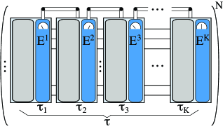
Figure 1: Multiple measurement and feedback scheme. The probe system (pictured as multiple qubits for simplicity) interacts with the external field and the control Hamiltonian during $K$ intervals each of length $\tau_{i}$ for a total time $\tau$ (gray rectangles). After each period a POVM measurement ($\left\{E_{\alpha}^{i}\right\}$) is performed on the system. Feedback is applied between each one of the $K$ steps based on the previous measurement outcome. The same scheme is then repeated $N$ times to improve statistics.

Proof – By inserting identity operators as POVMs at appropriate times, we may assume that every experiment run consists of $K$ measurements at times $\left\{\tau_{1},\,\tau_{2},....\tau_{K-1},\,\tau\right\}$ with POVMs given by $\left\{E_{\alpha}^{1}\right\},\,\left\{E_{\alpha}^{2}\right\},....\left\{E_{\alpha}^{K}\right\}$ respectively. Following the strategy used to prove Proposition 1, we would like to eliminate the explicit feedback loop and external Hamiltonian. For this purpose let the POVM be $E_{\beta}^{m}=\left(M_{\beta}^{m}\right)^{\dagger}M_{\beta}^{m}$ and the unitary evolution conditioned by feedback on the outcome $\left\{E_{\alpha_{1}}^{1},\,E_{\alpha_{2}}^{2},...E_{\alpha_{m-1}}^{m-1}\right\}$ be $U_{\alpha_{1},\alpha_{2},...,\alpha_{m-1}}$. By replacing $M_{\beta}^{m}$ with $U_{\alpha_{1},\alpha_{2},...,\alpha_{m-1}}M_{\beta}^{m}$ we can reproduce the feedback by applying a different set of POVM measurements. Also, we can set $H_{0}=0$ by going to the interaction picture with respect to $H_{0}$ and replacing $\rho_{in}$ with $e^{iH\tau_{1}}\rho_{in}e^{-iH\tau_{1}}$ and $M_{\alpha}^{L}$ with $e^{-iH_{0}\left(\tau_{L+1}-\tau_{L}\right)}M_{\alpha}^{L}$ (also $bH$ becomes time-dependent in the interaction picture). Overall any procedure involving feedback and a control Hamiltonian is equivalent to a different POVM and a time dependent $bH\left(t\right)$. We thus want to prove that this cannot give a better bound than the optimal POVM strategy.

Now we wish to calculate various uncertainties (see the Appendix) in terms of probabilities of various measurement outcomes. For zero external field the probability of the outcome $\left\{E_{\alpha_{1}}^{1},\,E_{\alpha_{2}}^{2},...E_{\alpha_{K}}^{K}\right\}$ is given by:

$$P_{0}\left\{E_{\alpha_{1}}^{1},\,E_{\alpha_{2}}^{2},...E_{\alpha_{K}}^{K}\right\}=Tr\left\{\rho_{in}E_{\alpha_{K}..\alpha_{1}}\right\},$$ (10)

where $E_{\alpha_{K}..\alpha_{L}}\equiv\left(M_{\alpha_{K}}...M_{\alpha_{L}}\right)^{\dagger}M_{\alpha_{K}}...M_{\alpha_{L}}$. For non-zero external field, to leading order in $b$ the change in the probability of a given outcome $P\left\{E_{\alpha_{1}}^{1},\,E_{\alpha_{2}}^{2},...E_{\alpha_{K}}^{K}\right\}$ is:

$$\delta P\left\{E_{\alpha_{1}}^{1},...,E_{\alpha_{K}}^{K}\right\}\cong\sum_{L=0}^{K-1}ib\left(\tau_{L}-\tau_{L-1}\right)\cdot Tr\left\{\left[A_{\alpha_{L}...\alpha_{1}}\rho_{in}\left(A_{\alpha_{L}..\alpha_{1}}\right)^{\dagger},\overline{H_{L}}\right]E_{\alpha_{K}..\alpha_{L+1}}\right\},$$ (11)

where $A_{\alpha_{L}..\alpha_{1}}\equiv M_{\alpha_{L}}...M_{\alpha_{1}}$ and $\overline{H_{L}}=\frac{\int_{\tau_{L}}^{\tau_{L+1}}H\left(t\right)}{\tau_{L+1}-\tau_{L}}$. Using the classical Fisher Information formulas given in the appendix we may write that:

$$\begin{array}[]{l}\left(\delta b_{min}^{2}\right)^{-1}=N\sum_{\alpha_{1},\alpha_{2},..\alpha_{K}}\frac{\left(\delta P\left\{E_{\alpha_{1}}^{1},\,E_{\alpha_{2}}^{2},...E_{\alpha_{K}}^{K}\right\}\right)^{2}}{b^{2}\,P_{0}\left\{E_{\alpha_{1}}^{1},\,E_{\alpha_{2}}^{2},...E_{\alpha_{K}}^{K}\right\}}=\\ =N\displaystyle{\sum_{L,M=0}^{K-1}}\sum_{\alpha_{1},\alpha_{2},..\alpha_{K}}\frac{\left(\tau_{L+1}-\tau_{L}\right)\cdot\left(\tau_{M+1}-\tau_{M}\right)}{Tr\left\{\rho_{in}E_{\alpha_{K}....\alpha_{1}}\right\}}Tr\left\{\left[A_{\alpha_{L}..\alpha_{1}}\rho_{in}\left(A_{\alpha_{L}...\alpha_{1}}\right)^{\dagger},\overline{H_{L}}\right]E_{\alpha_{K}..\alpha_{L+1}}\right\}\\ \qquad\qquad\qquad\qquad\cdot Tr\left\{\left[A_{\alpha_{L}..\alpha_{1}}\rho_{in}\left(A_{\alpha_{L}...\alpha_{1}}\right)^{\dagger},\overline{H_{L}}\right]E_{\alpha_{K}...\alpha_{M+1}}\right\}\end{array}$$

In the second step we have changed the order of summation. Applying the Cauchy-Schwartz inequality to the sum $\sum_{\alpha_{1}..\alpha_{K}}$ (to separate contributions corresponding to different POVM measurements) we obtain

$$\begin{array}[]{l}\delta b_{min}^{-2}\leq N\displaystyle{\sum_{L,M=0}^{K-1}}\left\{\left(\tau_{L+1}-\tau_{L}\right)\left(\tau_{M+1}-\tau_{M}\right)\left[\sum_{\alpha_{1}..\alpha_{K}}\frac{Tr\left\{\left[A_{\alpha_{L}...\alpha_{1}}\rho_{in}A_{\alpha_{L}..\alpha_{1}}^{\dagger},\overline{H_{L}}\right]E_{\alpha_{K}..\alpha_{L+1}}\right\}^{2}}{Tr\left\{\rho_{in}E_{\alpha_{K}...\alpha_{1}}\right\}}\right]^{1/2}\right.\\ \left.\qquad\qquad\qquad\qquad\>\left[\sum_{\alpha_{1}...\alpha_{K}}\frac{Tr\left\{\left[A_{\alpha_{L}..\alpha_{1}}\rho_{in}A_{\alpha_{L}..\alpha_{1}}^{\dagger},\overline{H_{L}}\right]E_{\alpha_{K}...\alpha_{M+1}}\right\}^{2}}{Tr\left\{\rho_{in}E_{\alpha_{K}....\alpha_{1}}\right\}}\right]^{1/2}\right\}\end{array}$$

Since the operator $A_{\alpha_{L}..\alpha_{1}}\rho_{in}A_{\alpha_{L}..\alpha_{1}}^{\dagger}\equiv s\rho_{\alpha_{L}..\alpha_{1}}$ is positive definite, up to a scaling factor $s$ it represents a density operator. Also we note that

$$Tr\left\{\rho_{in}E_{\alpha_{K}....\alpha_{1}}\right\}=Tr\left\{A_{\alpha_{L}..\alpha_{1}}\rho_{in}A_{\alpha_{L}..\alpha_{1}}^{\dagger}E_{\alpha_{K}..\alpha_{L+1}}\right\}$$

and that $\left\{E_{\alpha_{K}....\alpha_{L+1}}\right\}$ is a POVM. As a result, we can apply Proposition 3 to the normalized $A_{\alpha_{L}..\alpha_{1}}\rho_{in}A_{\alpha_{L}..\alpha_{1}}^{\dagger}$, obtaining

$$\begin{array}[]{l}\sum_{\alpha_{1}..\alpha_{K}}\frac{\left(Tr\left\{\left[A_{\alpha_{L}..\alpha_{1}}\rho_{in}A_{\alpha_{L}..\alpha_{1}}^{\dagger},\overline{H_{L}}\right]E_{\alpha_{K}..\alpha_{L+1}}\right\}\right)^{2}}{Tr\left\{\rho_{in}E_{\alpha_{K}....\alpha_{1}}\right\}}\\ \leq\sum_{\alpha_{1}..\alpha_{L}}\left(\Lambda-\lambda\right)Tr\left\{A_{\alpha_{L}..\alpha_{1}}\rho_{in}A_{\alpha_{L}..\alpha_{1}}^{\dagger}\right\}=\Lambda-\lambda\end{array}$$ (12)

The first inequality derives from Proposition 2 and the fact that the spread of eigenvalues of $\overline{H}$ is less then $\Lambda-\lambda$. The last equality is obtained by noting that $\sum_{\alpha_{1}..\alpha_{L}}A_{\alpha_{L}..\alpha_{1}}^{\dagger}A_{\alpha_{L}..\alpha_{1}}=\leavevmode\hbox{\small 1\normalsize\kern-3.30002pt1}$. Finally we obtain the bound

$$\delta b_{min}^{-2}\leq N{\displaystyle\sum_{L=0}^{K-1}\sum_{M=0}^{K-1}}\left(\tau_{L+1}-\tau_{L}\right)\left(\tau_{M+1}-\tau_{M}\right)\left(\Lambda-\lambda\right)^{2}=N\tau^{2}\left(\Lambda-\lambda\right)^{2}$$ (13)

We therefore conclude that multiple POVM rounds and feedback cannot improve the sensitivity beyond the limit given by Eq. (1).$\hfill\Box\vspace{8pt}$

Note that by choosing a set of POVMs $\{E_{\alpha_{1}},...,E_{\alpha_{L}}\}$ that maximizes the sum $\sum_{\alpha_{K}..\alpha_{L+1}}\frac{\left(Tr\left\{\left[\rho_{\alpha_{L}..\alpha_{1}},\overline{H_{L}}\right]E_{\alpha_{K}..\alpha_{L+1}}\right\}\right)^{2}}{Tr\left\{\rho_{\alpha_{L}..\alpha_{1}}E_{\alpha_{K}....\alpha_{L+1}}\right\}}$ we can find a single step in the multiple POVM sequence that is at least as efficient as the entire feedback sequence.

Proposition 4 – Bound for mixed states with feedback and multi-round measurements.
Suppose the system is initialized in the state $\rho_{in}$ and interacts with the Hamiltonian $b\,H+H_{0}$. During the evolution a set of POVMs $\left\{E_{\mu}^{1,i}\right\}$ are measured . Here $i$ stands for the POVM measurement number, $\mu$ is the outcome and $1$ identifies the first round of measurements. Feedback based on the measurement outcomes determines the control Hamiltonian and the choice of POVMs. The overall measurement procedure lasts a time $\tau$. The next round of measurement uses a potentially different initial state, a different set of POVMs $\left\{E_{\nu}^{2,j}\right\}$ and a different feedback scheme. Furthermore the second measurement procedure may depend on the results of the first measurement and also lasts a time $\tau$. A total of $N$ rounds of measurements are carried out, so that the total measurement time is given by $N\tau$ (see Fig. 2). The minimum uncertainty of $b$ obtained by this scheme is given by Eq. (1), $\delta b_{min}\geq\frac{1}{\tau\sqrt{N}\left(\Lambda-\lambda\right)}$.

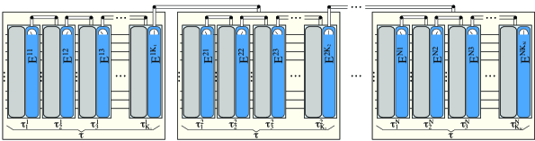
Figure 2: Multiple round measurement and feedback scheme (with classical communication between rounds). The probe system (pictured as multiple qubits for simplicity) undergoes $N$ measurement rounds each lasting a total time $\tau$. The evolution in each round $i$ is subdivided into $K_{i}$ intervals each of length $\tau_{j}^{i}$. During each interval, the system interacts with the external field and a control Hamiltonian (gray rectangle) that depends on feedback from the previous interval and the previous round. After each time interval, a POVM measurement $\left\{E_{\alpha}^{i,j}\right\}$ (chosen according to the feedback scheme) is performed on the system (blue rectangle). The result of the measurement is used to control the next time interval or the next measurement round.

Proof – By Corollary 4 (see Appendix) we know that $\delta b_{min}^{2}\geq\left[{\sum_{1\rightarrow N}\frac{\left(\delta P\left(O_{\alpha}^{1\rightarrow N}\right)\right)^{2}}{P_{0}\left(O_{\alpha}^{1\rightarrow N}\right)}}\right]^{-1}$, where the sum is over all possible outcomes $O_{\alpha}^{1\rightarrow N}$ of the $N$ rounds of POVM measurements. We wish to prove by induction on $N$ that $\left(\delta b_{min}^{2}\right)^{-1}\leq N\tau^{2}\left(\Lambda-\lambda\right)^{2}$. The case $N=1$ is given by Proposition 3. If we assume that $\sum_{1\rightarrow N-1}\frac{\left(\delta P\left(O_{\alpha}^{1\rightarrow N-1}\right)\right)^{2}}{P_{0}\left(O_{\alpha}^{1\rightarrow N-1}\right)}\leq\left(N-1\right)\tau^{2}\left(\Lambda-\lambda\right)^{2}$, we obtain the bound:

$$\begin{array}[]{l}\sum_{1\rightarrow N}\frac{\left(\delta P\left(O_{\alpha}^{1\rightarrow N}\right)\right)^{2}}{P_{0}\left(O_{\alpha}^{1\rightarrow N}\right)}=\sum_{1\rightarrow N-1}\sum_{N}\left(\frac{\left(\delta P\left(O_{\beta}^{1\rightarrow N-1}\right)\cdot P_{0}\left(O_{\gamma}^{N}\right)+\delta P\left(O_{\beta}^{1\rightarrow N-1}\right)\cdot P_{0}\left(O_{\gamma}^{N}\right)\right)^{2}}{P_{0}\left(O_{\alpha}^{1\rightarrow N-1}\right)\cdot P_{0}\left(O_{\gamma}^{N}\right)}\right)\\ =\sum_{1\rightarrow N-1}\sum_{N}\left\{\frac{\left(\delta P\left(O_{\beta}^{1\rightarrow N-1}\right)\right)^{2}\cdot P_{0}\left(O_{\gamma}^{N}\right)}{P_{0}\left(O_{\beta}^{1\rightarrow N-1}\right)}+\frac{\left(\delta P\left(O_{\alpha}^{N}\right)\right)^{2}\cdot P_{0}\left(O_{\beta}^{1\rightarrow N-1}\right)}{P_{0}\left(O_{\alpha}^{N}\right)}\right\}\leq N\tau^{2}\left(\Lambda-\lambda\right)^{2}\end{array}$$ (14)

Here the outcome $O_{\alpha}^{1\rightarrow N}$ is given by the outcomes $O_{\beta}^{1\rightarrow N-1}$ in the first $N-1$ rounds of measurement and $O_{\gamma}$ in the last round. The first equality holds because the probability of the last measurement outcome is independent of the previous measurements. The second equality derives from $\sum\delta P\left(O_{\alpha}^{N}\right)=0$. Finally, by noting that $\sum P_{0}\left(O_{\alpha}^{N}\right)=\sum P_{0}\left(O_{\beta}^{1\rightarrow N-1}\right)=1$, we can obtain by induction the last inequality.$\hfill\Box\vspace{8pt}$

This result indicates that classical communication between different measurement rounds cannot improve sensitivity beyond the limit given in Eq. (1). Specifically, the “independence” of the uncertainties between steps of the multi-round strategy (demonstrated in Eq. 14) indicates that the sensitivity obtained by choosing one of the measurement rounds is at least as high as that of the overall procedure.

VI Example: Sensitivity Improvement with Auxiliary Qubits

We now present an illustration of the bounds derived in this paper, in particular the effects of an ancillary system and an external control field. In many experimental situations key-20 ; key-21 a probe consists of a quantum sensor (for simplicity a two-level system) and a spin environment. The external field, which we wish to measure, is coupled to both the sensor and the environment. The sensitivity of the probe can then be enhanced by using the environment spins as ancillas to enhance the response of the system to the external field.

We assume that the sensor spin (which can be prepared in a well defined initial state, coherently manipulated and read out) is coupled to a bath of “dark” spins, which can be polarized and collectively controlled but cannot be directly detected. The system is described by the Hamiltonians:

$$\begin{array}[]{l}H=H_{meas}+H_{int}\\ H_{int}=\left|1\right\rangle\left\langle 1\right|\lambda{\displaystyle\sum I_{x}^{i}},\>H_{meas}=b\left(\left|1\right\rangle\left\langle 1\right|+{\displaystyle\sum I_{z}^{i}}\right),\end{array}$$ (15)

where $\lambda$ is the coupling between the sensor and environment spins. Here $\left|0\right\rangle,\,\left|1\right\rangle$ refer to the sensor spin while $\left|\uparrow\right\rangle,\,\left|\downarrow\right\rangle,\,I_{z}^{i}$ describe the dark spins. We shall consider the case where $H_{int}$ can be turned on and off at will and is much larger in magnitude then any other interaction in the system. As the spread of eigenvalues of $H_{meas}$ is equal to $1+K$ (where $K$ is the total number of ancillary spins) in principle it should be possible to attain Heisenberg limited metrology (with sensitivity scaling $\sim\frac{1}{K}$) using this Hamiltonian. This is very similar to metrology using GHZ states or systems with multi-body coupling to the parameter key-27 (29).

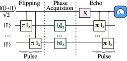
Figure 3: A quantum circuit used to enhance parameter estimation sensitivity. CNOT gates make the state of the dark spins dependent on the state of the sensor spin. The dark spins pick up different phases dependent on the state of the sensor spin and the echo followed by more CNOT gates maps this phase onto the sensor spin which is then read out. Here $\tau_{pulse}=\frac{\pi}{2\lambda}$, $X$ stands for a $\pi$ pulse on the sensor qubit flipping $\left|0\right\rangle\leftrightarrow\left|1\right\rangle$.

To illustrate this method we consider the idealized case when the coupling between the sensor spin and the dark spins are in our control and the dark spins are initialized in a pure state: $\left|\uparrow...\uparrow\right\rangle$. Consider the circuit shown in Fig. 3. First, the sensor spin is prepared in an equal superposition of the two internal states $\left|0\right\rangle+\left|1\right\rangle$ (dropping normalization). Then $H_{int}$ (CNOT gates on the dark spins) is used to produce the state:

$$\left|0\right\rangle\left|\uparrow...\uparrow\right\rangle+\left|1\right\rangle\left|\downarrow...\downarrow\right\rangle,$$ (16)

This state is then used to sense the magnetic field. The action of the external field leads to the states $\left|0\right\rangle\left|\uparrow...\uparrow\right\rangle$ and $\left|1\right\rangle\left|\downarrow...\downarrow\right\rangle$ acquiring different phases $\tau\frac{K+2}{2}$ and $-\tau\frac{K}{2}$, respectively. After the interaction with the magnetic field, the sensor spin is flipped and another control operation with $H_{int}$ is applied. This leads to the following final state for the total spin system:

$$\left(e^{-i\tau b\left(1+\frac{K}{2}\right)}\left|1\right\rangle+e^{\frac{i\tau bK}{2}}\left|0\right\rangle\right)\left|\downarrow...\downarrow\right\rangle$$ (17)

Note that this is a product state of the sensor spin and the dark spin states. If we then measure the operator $\mathcal{O\equiv}i\left(\left|0\right\rangle\left\langle 1\right|-\left|1\right\rangle\left\langle 0\right|\right)$ (say $N$ times to improve statistics) we would get a minimum uncertainty $b_{min}\doteq\sqrt{\frac{1}{N}}\frac{1}{\left(1+K\right)\tau}$ (or Heisenberg limited metrology). This effect may be understood by noting that the circuit shown in Fig. 2 effectively converts the measurement Hamiltonian $H_{meas}\equiv b\left(\left|1\right\rangle\left\langle 1\right|+{\displaystyle\sum I_{z}^{i}}\right)$ to a new interaction $\widetilde{H}_{meas}\equiv b\left|1\right\rangle\left\langle 1\right|\left(\mathbb{I}+{\displaystyle\sum I_{z}^{i}}\right)$. This new Hamiltonian is much more convenient, since it is possible to prepare the optimal initial state, $\frac{1}{\sqrt{2}}\left(\left|0\right\rangle+\left|1\right\rangle\right)\left|\downarrow...\downarrow\right\rangle$ (which is a an equal superposition of the two eigenstates with largest and smallest eigenvalues) and measure the optimal operator for this state and Hamiltonian, $i\left(\left|0\right\rangle\left\langle 1\right|-\left|1\right\rangle\left\langle 0\right|\right)$ (see Corollary 3 in the Appendix).

VII Conclusions

In this work we have presented a new proof of the Cramer-Rao bound and extended the bound to more general metrology frameworks, encompassing e.g. feedback. Key to our proof was the realization that more complex metrology schemes cannot improve on the ideal parameter estimation performed via a two-level systems with the optimal initial state and observable. Using only Cauchy-Schwartz inequalities and the Fisher Information, we proved that the sensitivity cannot increase, even when adding external control, ancillary systems, using mixed states and POVM measurements as well as multiple rounds of measurements with feedback.

Specifically, we systematically increased the complexity of the metrology procedure, by introducing one by one additional features often considered in the literature and in experiments. The new metrology scheme obtained at each step is composed of many sub-procedures that have been considered in the previous scheme; we were thus always able to identify a sub-procedure that provided as high a sensitivity as the more complex metrology scheme. By backward induction, it is then possible to explicitly construct a two-level system, initialized in a pure state, with no control Hamiltonians and a single operator measurement that is a sub-step of the more complex measurement procedure but is as efficient –or more– than the whole measurement process. Although this ideal simple system is not always experimentally accessible, and thus more complex strategies need to be adopted in practice, we showed that when constrained by a given sensing time, none of these strategies can surpass the fundamental Cramer-Rao limit.

Appendix A General Sensitivity Formulas

For sake of completeness we present a known result —the classical Fisher Information key-1 ; key-2 ; key-3 — that has been used extensively in the main text of the paper. We show that maximum likelihood estimates saturate the Fisher information bound in the limit of an infinite number of measurements and we demonstrate the bound for finite number of measurements.

Lemma 3 – Generic bounds for parameter estimation.
Consider a generic system coupled to some external field. The system interacts with the field and potentially other control Hamiltonians. It is possible that multiple sensing sequences are carried out on the system; that is several sets of POVMs $\left\{E_{\mu}^{1}\right\}...\left\{E_{\nu}^{m}\right\}$ are measured. The process is repeated $N$ times to improve statistics. Suppose that $P\left(O_{\alpha}\right)\cong P_{0}\left(O_{\alpha}\right)+b\delta P\left(O_{\alpha}\right)$ (that is non-linear terms are negligible) where $P_{0}\left(O_{\alpha}\right)$ is the probability of measuring outcome $\alpha$ (which may be the result of several POVMs) for zero external field. Then in the limit $N\rightarrow\infty$ the minimum uncertainty for measuring the external field is given by the classical Fisher Information:

$$\delta b_{min}^{2}=\left[{N\sum\frac{\left(\delta P\left(O_{\alpha}\right)\right)^{2}}{P_{0}\left(E_{\alpha}\right)}}\right]^{-1}$$ (18)

Furthermore if only one POVM measurement $\left\{E_{\alpha}\right\}$ is made, this sensitivity can also be obtained by measuring the operator:

$$\mathcal{O}\equiv\sum\frac{E_{\alpha}}{P_{0}\left(E_{\alpha}\right)}$$ (19)

Proof – We will begin by calculating the probabilities of various outcomes of the measurements. After $N$ samplings the probability of observing $F_{\alpha}$ frequency of each of the possible outcomes $O_{\alpha}$ is given by:

$$P\left(F_{1},...F_{K}\right)=\frac{N!}{\left(F_{1}\cdot N\right)!\cdot\cdot\cdot\left(F_{K}\cdot N\right)!}\Pi_{\alpha=1}^{K}\left(P\left(O_{\alpha}\right)\right)^{NF_{\alpha}}\cong Exp\left[-\frac{N}{2}\Sigma\frac{\left(P\left(O_{\alpha}\right)-F_{\alpha}\right)^{2}}{P\left(O_{\alpha}\right)}\right]$$ (20)

Now we wish to isolate the part of Eq. (20) that depends on the external field $b$. Substituting $\Delta_{\alpha}\equiv F_{\alpha}-P_{0}\left(E_{\alpha}\right)$ we may write that:

$$\begin{array}[]{l}P\left(\Delta_{1},...\Delta_{K}\right)\cong Exp\left[-\frac{N}{2}\Sigma\frac{\left(P\left(O_{\alpha}\right)-F_{\alpha}\right)^{2}}{P\left(O_{\alpha}\right)}\right]=Exp\left[-\frac{N}{2}\Sigma\frac{\left(\frac{\Delta_{\alpha}}{\delta P\left(O_{\alpha}\right)}-b\right)^{2}\left(\delta P\left(O_{\alpha}\right)\right)^{2}}{P_{0}\left(O_{\alpha}\right)}\right]=\\ Exp\left[-\frac{N}{2}\sum\frac{\left(\delta P\left(E_{\alpha}\right)\right)^{2}}{P_{0}\left(E_{\alpha}\right)}\left(b-\frac{\sum\frac{\delta P\left(O_{\alpha}\right)}{P_{0}\left(O_{\alpha}\right)}\cdot\Delta_{\alpha}}{\sum\frac{\left(\delta P\left(O_{\alpha}\right)\right)^{2}}{P_{0}\left(O_{\alpha}\right)}}\right)^{2}\right]\cdot Exp\left[\sum\frac{\Delta_{\alpha}^{2}}{P_{0}\left(E_{\alpha}\right)}-\frac{\left[\sum\frac{\delta P\left(O_{\alpha}\right)}{P_{0}\left(O_{\alpha}\right)}\cdot\Delta_{\alpha}\right]^{2}}{\sum\frac{\left(\delta P\left(O_{\alpha}\right)\right)^{2}}{P_{0}\left(O_{\alpha}\right)}}\right]\end{array}$$ (21)

Qualitatively the second exponential after the last equality has no $b$ dependence so cannot provide any further information about the external field. This statement is made more quantitative in the following sublemma.

Sublemma 1 – The best possible estimate for $b$ is given by $b_{opt}\cong\frac{\sum\frac{\delta P\left(E_{\alpha}\right)\Delta_{\alpha}}{P_{0}\left(E_{\alpha}\right)}}{\sum\frac{\left(\delta P\left(E_{\alpha}\right)\right)^{2}}{P_{0}\left(E_{\alpha}\right)}}$ (which is the maximum likelihood estimate) with uncertainty $\delta b_{opt}\cong\frac{1}{\sqrt{N\sum\frac{\left(\delta P\left(E_{\alpha}\right)\right)^{2}}{P_{0}\left(E_{\alpha}\right)}}}$. For a single POVM $\left\{E_{\alpha}\right\}$ this estimate can be obtained by measuring the expectation of the operator $b=\left\langle\widetilde{\mathcal{O}}\right\rangle\equiv\frac{1}{\sum\frac{\left(\delta P\left(E_{\alpha}\right)\right)^{2}}{P_{0}\left(E_{\alpha}\right)}}\left\langle\sum\left(\frac{E_{\alpha}}{P_{0}\left(E_{\alpha}\right)}-1\right)\right\rangle$. Note that $\widetilde{\mathcal{O}}$ is the same as $\mathcal{O}$ in Eq. (19) up to a constant and rescaling.

Proof – We note that the expectation of the operator is indeed $b$ see Eq. (21). For fixed $b$ the expectation value of the operator $\widetilde{\mathcal{O}}$ comes from a Gaussian distribution centered at $b$ of width $\frac{1}{\sqrt{N\sum\frac{\left(\delta P\left(O\alpha\right)\right)^{2}}{P_{0}\left(O_{\alpha}\right)}}}$. As such we see that $\delta b_{opt}\leq\delta b_{\mathcal{O}}=\frac{1}{\sqrt{N\sum\frac{\left(\delta P\left(O_{\alpha}\right)\right)^{2}}{P_{0}\left(O_{\alpha}\right)}}}$. We would like to show that this is indeed optimal. Let $S$ be any statistic for $b$, that is a map of the frequency set onto $b$: $S:\left(F_{1},...F_{K}\right)\rightarrow b$. The uncertainty for this statistic is given by:

$$\begin{array}[]{l}\delta S^{2}=\lim_{L\rightarrow\infty}\frac{1}{2L}\intop_{-L}^{L}db\iiint dF_{1}..dF_{K}P\left(F_{1}..F_{K}\mid b\right)\cdot\left(b-S\left(F_{1},...F_{K}\right)\right)^{2}=\\ \lim_{L\rightarrow\infty}\frac{1}{2L}\iiint dF_{1}..dF_{K}\intop_{-L}^{L}db\cdot G\left(F_{1}..F_{K}\right)\cdot\left(b-S\left(F_{1},...F_{K}\right)\right)^{2}\cdot Exp\left[-\frac{\Lambda}{2}\left(b-\Delta\right)^{2}\right]=\\ \lim_{L\rightarrow\infty}\frac{1}{2L}\iiint dF_{1}..dF_{K}\intop_{-L}^{L}db\cdot G\left(F_{1}..F_{K}\right)\cdot\left(\frac{1}{\Lambda}+\left(b-S\left(F_{1},...F_{K}\right)\right)^{2}\right)\geq\frac{1}{\Lambda}\end{array}$$ (22)

Here $\Delta={\sum\frac{\delta P\left(O\alpha\right)\Delta_{\alpha}}{P_{0}\left(O_{\alpha}\right)}}/{\sum\frac{\left(\delta P\left(O_{\alpha}\right)\right)^{2}}{P_{0}\left(O_{\alpha}\right)}}$, $G\left(F_{1}..F_{K}\right)=Exp\left[\sum\frac{\Delta_{\alpha}^{2}}{P_{0}\left(O_{\alpha}\right)}-\frac{\left[\sum\frac{\delta P\left(O_{\alpha}\right)}{P_{0}\left(O\alpha\right)}\cdot\Delta_{\alpha}\right]^{2}}{\sum\frac{\left(\delta P\left(O_{\alpha}\right)\right)^{2}}{P_{0}\left(O_{\alpha}\right)}}\right]$ and $\Lambda=N\sum\frac{\left(\delta P\left(O_{\alpha}\right)\right)^{2}}{P_{0}\left(O_{\alpha}\right)}$ (see Eq. (21)). In the first step we have changed the order of integration, in the second we have used well know properties of Gaussian integrals and for the third note that $\left(b-S\left(F_{1},...F_{K}\right)\right)^{2},\ G\left(F_{1}..F_{K}\right)\geq 0$. In particular for one POVM measurement any statistic no more efficient then measuring $\widetilde{\mathcal{O}}$ or equivalently $\mathcal{O}$. $\hfill\Box\vspace{8pt}$

We thus proved the uncertainty bound in Eq. (18).$\hfill\Box\vspace{8pt}$

Corollary 3 –Optimal observable.
Consider parameter estimation using the hypothesis in Corollary 1. The Cramer-Rao bound, Eq. (1), cannot be violated by measuring an operator instead of a POVM but it can be saturated by the measurement of a single observable $\mathcal{O}$, for appropriate initial states.

Proof – First, measuring an operator cannot be more efficient than measuring a POVM, as for any operator a POVM made of its eigenvalues is completely equivalent. Second, given an operator $\mathcal{O}$, the precision with which $b$ can be determined is given by:

$$\delta b=\frac{\Delta\mathcal{O}}{\sqrt{N}|\partial Tr\left\{\rho\mathcal{O}\right\}/\partial b|}\approx\frac{\Delta\mathcal{O}}{\tau\sqrt{N}\left|Tr\left\{\rho\left[H,\mathcal{O}\right]\right\}\right|},$$ (23)

where the second line is obtained by first order perturbation theory and $\Delta\mathcal{O}\equiv\sqrt{Tr\left\{\rho\mathcal{O}^{2}\right\}-\left(Tr\left\{\rho\mathcal{O}\right\}\right)^{2}}$. Explicitly if we choose $\mathcal{O}=i\left|\Lambda\right\rangle\left\langle\lambda\right|-i\left|\lambda\right\rangle\left\langle\Lambda\right|$ and $\left|\Psi\right\rangle=\frac{1}{\sqrt{2}}\left(\left|\Lambda\right\rangle+\left|\lambda\right\rangle\right)$, ($\rho=\left|\Psi\right\rangle\left\langle\Psi\right|$) we obtain $\frac{\left|\left\langle\Psi\right|\left[H,\mathcal{O}\right]\left|\Psi\right\rangle\right|}{\left\langle\Delta\mathcal{O}\right\rangle}=\Lambda-\lambda$.$\hfill\Box\vspace{8pt}$

Corollary 4 – Generic bounds for parameter estimation with finite number of trials. Consider a generic system coupled to some external field.
The system interacts with the field and potentially other control Hamiltonians. Possibly multiple sensing sequences are carried out on the system that is several sets of POVMs $\left\{E_{\alpha}^{1}\right\}...\left\{E_{\alpha}^{k}\right\}$ are measured. The process is repeated $K$ times to improve statistics. Suppose that $P\left(O_{\alpha}\right)\cong P_{0}\left(O_{\alpha}\right)+b\delta P\left(O_{\alpha}\right)$ where $P_{0}\left(O_{\alpha}\right)$ is the probability of measuring outcome $\alpha$ (which may be the result of several POVMs) for zero external field. Then for any $K$ measurements the minimum uncertainty for measuring the external field is given by:

$$\delta b_{min}^{2}\geq\frac{1}{K\sum\frac{\left(\delta P\left(O_{\alpha}\right)\right)^{2}}{P_{0}\left(O_{\alpha}\right)}}$$ (24)

Here $K$ is a finite number of repetitions of the experiment used to improve statistics. In particular if the measurement is carried out only once $\delta b_{min}^{2}\geq\frac{1}{\sum\frac{\left(\delta P\left(O_{\alpha}\right)\right)^{2}}{P_{0}\left(O_{\alpha}\right)}}$.

Proof – Consider any statistic ($S$) used to determine $b$ using $K$ measurements, let it have uncertainty $\Delta_{K}$. Now consider repeating this experiment $N\rightarrow\infty$ times (for a total of $N\cdot K$ measurements). By Lemma 2 we know that the optimum measurement produces uncertainty $\delta b_{opt}=\frac{1}{\sqrt{NK\sum\frac{\left(\delta P\left(O_{\alpha}\right)\right)^{2}}{P_{0}\left(O_{\alpha}\right)}}}$. On the other hand taking the average of $N$ copies of statistic $S$ leads to uncertainty $\delta b_{opt}\leq\delta b_{NK}=\frac{1}{\sqrt{N}\Delta_{K}}$. From this we see that $\Delta_{K}\geq\frac{1}{\sqrt{K\sum\frac{\left(\delta P\left(O_{\alpha}\right)\right)^{2}}{P_{0}\left(O_{\alpha}\right)}}}$ and Eq. (24) follows. $\hfill\Box\vspace{8pt}$

Acknowledgments – This work was supported by NSF and the Packard Foundation. P.C. was in part supported by an ITAMP fellowship.

References

(1) Braunstein S L and Caves C M 1994 Phys. Rev.
Lett.72 3439
(2) Braunstein S L, Caves C M and Milburn G J 1996 Ann.
Phys. (N.Y.)247 135
(3)Cramer H 1946 Mathematical Methods of Statistics
(Princeton: Princeton University Press)
(4) Jozsa R, Abrams D S, Dowling J P and Williams C P
2000 Phys. Rev. Lett.85 2010
(5) Chuang I L 2000 Phys. Rev. Lett.85
2006
(6) Wineland D J, Bollinger J J, Itano W M, Moore
F L and Heinzen D J 1992 Phys. Rev. A46 R6797
(7) Giovannetti V, Lloyd S and Maccone L 2006
Phys. Rev. Lett. 96 010401
(8) Revzen M and Mann A 2003 Phys. Lett. A312
11
(9) de Burgh M and Bartlett S D 2005 Phys. Rev.
A72 042301
(10) Boixo S, Caves C M, Datta A and Shaji A 2006
Laser Phys.16 1525
(11) Bagan E, Baig M and Tapia R M 2001 Phys.
Rev. Lett.87 257903
(12) Chiribella G, D’Ariano G M, Perinotti P and Sacchi
M F 2004 Phys. Rev. Lett.93 180503
(13) Gerry C C and Campos R A 2003 Phys. Rev.
A68 025602
(14) Dunningham J A and Burnett K 2004 Phys.
Rev. A70 033601
(15) Wang H and Kobayashi T 2005 Phys. Rev. A71 021802(R)
(16) Rosenband T, Hume D B, Schmidt P O, Chou C W, Brusch
A, Lorini L, Oskay W H, Drullinger R E, Fortier T M, Stalnaker J E
et al. 2008 Science319 1808
(17) Rosenband T, Schmidt P O, Hume D B, Itano W M, Fortier
T M, Stalnaker J E, Kim K, Diddams S A, Koelemeij J C J, Bergquist
J C et al. 2007 Phys. Rev. Lett.98 220801
(18) Oskay W H, Diddams S A, Donley E A, Fortier T M,
Heavner T P, Hollberg L, Itano W M, Jefferts S R, Delaney M J, Kim
K et al. 2006 Phys. Rev. Lett.97 020801
(19) Schmidt P O, Rosenband T, Langer C, Itano W M, Bergquist
J C and Wineland D J 2005 Science309 749
(20) Giovannetti V, Lloyd S and Maccone L 2004 Science306 1330
(21) Giovannetti V, Lloyd S and Maccone L 2002 Phys.
Rev. A65, 022309
(22) Taylor J M, Cappellaro P, Childress L, Jaing L,
Budker D, Hemmer P R, Yacoby A, Walsworth R and Lukin M D 2008 Nat.
Phys.4 810
(23) Maze J R, Stanwix P L, Hodges J S, Hong S, Taylor
J M, Cappellaro P, Jaing L, Gurudev Dutt M V, Togan E, Zibrov A S
et al. 2008 Nature455 644
(24) Jiang L, Hodges J S, Maze J R, Maurer P, Taylor
J M, Cory D G, Hemmer P R, Walsworth R L, Yacoby A, Zibrov A S et
al. 2009 Science326 267
(25) Geremia J M, Stockton J K, Doherty J C and Mabuchi
H 2003 Phys. Rev. Lett.91 250801
(26) Stockton J K, Geremia J M, Doherty J C and Mabuchi
H 2004 Phys. Rev. A69 032109
(27) Bollinger J J, Itano W M, Wineland D J and Heinzen
D J 1996 Phys. Rev. A54 R4649
(28) Gel’fand I M 1961 Lectures on Linear
Algebra (Interscience Tracts in Pure and Applied Mathematics) ed
L Bers, R Courant et al. (New York: Interscience Publishing
Inc.)
(29)Boixo S, Flamia S T, Caves C M and Geremia J
M 2007 Phys. Rev. Lett.98 090401