CERN-PH-TH/2010-014

Extra Dimensions at the LHC

Kyoungchul Kong ^a, Konstantin Matchev ^b and Géraldine Servant ^c,d

^a Theoretical Physics Department, SLAC, Menlo Park, CA 94025, USA
^b Physics Department, University of Florida, Gainesville, FL 32611, USA
^c CERN Physics Department, Theory Division, CH-1211 Geneva 23, Switzerland
^d Institut de Physique Théorique, CEA Saclay, F91191 Gif-sur-Yvette, France

Abstract

We discuss the motivation and the phenomenology of models with either flat or warped extra dimensions. We describe the typical mass spectrum and discovery signatures of such models at the LHC. We also review several proposed methods for discriminating the usual low-energy supersymmetry from a model with flat (universal) extra dimensions.

From ‘Particle Dark Matter: Observations, Models and Searches’
edited by Gianfranco Bertone
Copyright $@$ 2010 Cambridge University Press.
Chapter 15, pp. 306-324, Hardback ISBN 9780521763684, http://cambridge.org/us/catalogue/catalogue.asp?isbn=9780521763684

1 Extra Dimensions at the LHC

In models with extra dimensions, the usual $3+1$ dimensional space-time $x^{\mu}\equiv(x^{0},x^{1},x^{2},x^{3})$ is extended to include additional spatial dimensions parameterized by coordinates $x^{4},x^{5},\ldots,x^{3+N}$. Here $N$ is the number of extra dimensions. String theory arguments would suggest that in principle $N$ can be as large as 6 or 7. In this chapter, we are interested in extra dimensional (ED) models where all particles of the Standard Model (SM) are allowed to propagate in the bulk, i.e. along any of the $x^{3+i}$ $(i=1,\ldots,N)$ directions [1]. In order to avoid a blatant contradiction with the observed reality, the extra dimensions in such models must be extremely small: smaller than the smallest scale which has been currently resolved by experiment. Therefore, the extra dimensions are assumed to be suitably compactified on some manifold of sufficiently small size (see Fig. 1).

Depending on the type of metric in the bulk, the ED models fall into one of the following two categories: flat, a.k.a. “universal” extra dimensions (UED) models, discussed in Section 2, or warped ED models, discussed in Section 3. As it turns out, the collider signals of the ED models are strikingly similar to the signatures of supersymmetry (SUSY) [2]. Section 4 outlines some general methods for distinguishing an ED model from SUSY at high energy colliders.

2 Flat extra dimensions (UED)

2.1 Definition

In this section, we choose the metric on the extra dimensions to be flat. For simplicity, we shall limit our discussion to models with $N=1$ or $N=2$ UEDs. In the simplest case of $N=1$, a compact extra dimension $x^{4}$ would have the topology of a circle $S^{1}$. However, in order to implement the chiral fermions of the SM in a UED framework, one must use a manifold with endpoints, e.g. the orbifold $S^{1}/Z_{2}$, pictorially represented in Fig. 1(a). The opposite sides of the circle are identified, as indicated by the black vertical arrows. The net result is a single line segment with two endpoints, denoted by the blue dots. The size of the extra dimension in this case is simply parameterized by the radius of the circle $R$.

1.5 1.0   

Figure 1: (a) Compactification of $N=1$ extra dimension on a circle with opposite points identified. (b) Compactification of $N=2$ extra dimensions on the chiral square with adjacent sides identified. In each case, the black arrows indicate the corresponding identification. The blue dots represent fixed (boundary) points.

In the case of two extra dimensions ($N=2$) there are several possibilities for compactification. One of them is the so called “chiral square” and corresponds to a $T^{2}/Z_{4}$ orbifold [3]. It can be visualized as shown in Fig. 1(b). The two extra dimensions have equal size, and the boundary conditions are such that the adjacent sides of the “chiral square” are identified, as indicated by the black arrows. The resulting orbifold endpoints are again denoted by blue dots.

An important concept in any UED model is the notion of Kaluza-Klein (KK) parity, whose origin can be traced back to the geometrical symmetries of the compactification. For example, in the $N=1$ case of Fig. 1(a), KK-parity corresponds to the reflection symmetry with respect to the center of the line segment. Similarly, in the $N=2$ case of Fig. 1(b), KK parity is due to the symmetry with respect to the center of the chiral square. In general, UED models respect KK parity, and this fact has important consequences for their collider and astroparticle phenomenology.

2.2 Mass spectrum

Since the extra dimensions are compact, the extra-dimensional components of the momentum of any SM particle are quantized in units of $\frac{1}{R}$. From the usual 4-dimensional point of view, those momentum components are interpreted as masses. Therefore in UED models each SM particle is accompanied by an infinite tower of heavy KK particles with masses $\frac{n}{R}$, where the integer $n$ counts the number of quantum units of extra-dimensional momentum. All KK particles at a given $n$ are said to belong to the $n$-th KK level, and at leading order appear to be exactly degenerate.

However, the masses of the KK particles receive corrections from several sources, which will lift this degeneracy. First, there are tree-level corrections arising from electroweak symmetry breaking through the usual Higgs mechanism. More importantly, there are one-loop mass renormalization effects due to the usual SM interactions in the bulk [4]. Finally, there may be contributions from boundary terms which live on the orbifold fixed points (the blue dots in Fig. 1) [4, 5]. In the so-called “minimal UED” models, the last effect is ignored and the resulting one-loop radiatively corrected spectrum of the first level KK modes is as shown in Fig. 2.

    

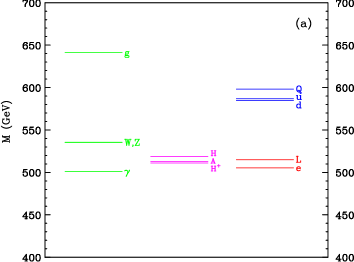
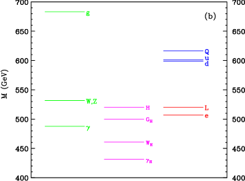
Figure 2: The radiatively corrected mass spectrum of the level one ($n=1$) KK particles in the two UED models from Fig. 1, for $R^{-1}=500$ GeV. In each panel, from left to right we list the KK particles of spin-1 (green), spin-0 (magenta) and spin-$\frac{1}{2}$ (blue for KK quarks and red for KK leptons). Figures taken from Refs. [4] and [6].

In the case of $N=1$ minimal UED shown in Fig. 2(a), we find that the SM particle content is simply duplicated at the $n=1$ level. The mass splittings among the KK particles arise mainly due to radiative corrections, which are largest for the colored particles (KK quarks and KK gluon). The lightest KK particle (LKP) at level one in this case is denoted by $\gamma_{1}$ and represents a linear superposition of the KK modes of the hypercharge gauge boson $B_{1}$ and the neutral component of the $SU(2)$ gauge boson $W^{0}_{1}$.

Fig. 2(b) reveals that the $n=1$ KK mass spectrum is somewhat more complex in the case of 2 extra dimensions ($N=2$). This is because gauge bosons propagating in 5+1 dimensions may be polarized along either of the two extra dimensions. As a result, for each spin-1 KK particle associated with a gauge boson, there are two spin-0 fields transforming in the adjoint representation of the gauge group. One linear combination of those becomes the longitudinal degree of freedom of the spin-1 KK particle, while the other linear combination remains as a physical spin-0 particle, called the spinless adjoint. In Fig. 2(b) the spinless adjoints are designated by an index “H”. Fig. 2(b) also reveals that in the minimal $N=2$ UED model, the LKP is the spinless photon $\gamma_{\rm H}$ [7, 6].

2.3 Collider signals

In terms of the KK level number $n$, KK parity can be simply defined as $(-1)^{n}$. The usual Standard Model particles do not have any extra-dimensional momentum, and therefore have $n=0$ and positive KK parity. On the other hand, the KK particles can have either positive or negative KK parity, depending on the value of $n$. Notice that the lightest KK particle at $n=1$ (i.e. the LKP) has negative KK parity and is absolutely stable, since KK parity conservation prevents it from decaying into SM particles. The collider phenomenology of the UED models is therefore largely determined by the nature of the LKP. In both of the minimal UED models shown in Fig. 2, the LKP is a neutral weakly interacting particle, whose signature will be missing energy in the detector. At hadron colliders the total parton level energy in the collision is a priori unknown, hence the presence of LKP particles in the event must be inferred from an imbalance in the total transverse momentum.

The collider phenomenology of the minimal UED models from Fig. 2 has been extensively investigated at both linear colliders [8, 9, 10, 11, 12, 13, 14] and hadron colliders [15, 16, 2, 17, 6, 18, 13, 19]. Due to KK parity conservation, the KK particles are always pair-produced, and then each one undergoes a cascade decay to the LKP, as illustrated in Fig. 3 [2, 18]. It is interesting to notice that the decay patterns in UED look very similar to those arising in R-parity conserving supersymmetry. The typical UED signatures include a certain number of jets, a certain number of leptons and photons, plus missing energy $\not\!\!E_{T}$.

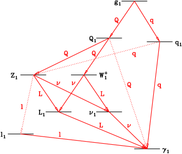
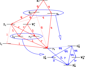
Figure 3: Qualitative sketch of the level 1 KK spectroscopy depicting the dominant (solid) and rare (dotted) transitions and the corresponding decay product for the $N=1$ (left) and $N=2$ (right) UED models from Fig. 2. Figures taken from Refs. [2] and [12].

Which particular signature among all these offers the best prospects for discovery? The answer to this question depends on the interplay between the predicted signal rates in UED and the expected SM backgrounds. For example, at lepton colliders the SM backgrounds are firmly under control, and the best channel is typically the one with the largest signal rate. Since at lepton colliders the new particles are produced through the same (electroweak) interactions, the largest rates are associated with the lightest particles in the spectrum - the KK leptons and the electroweak KK gauge bosons. In contrast, at hadron colliders the dominant production is through strong interactions, and the largest cross-sections belong to the colored KK particles, which typically decay through jets. Unfortunately, the SM QCD backgrounds to the jetty UED signatures are significant, and in that case there is a substantial benefit in looking for leptons instead. As seen in Fig. 3, the decays of the weakly interacting KK quarks $Q_{1}$ proceed through $SU(2)$ KK gauge bosons $W^{\pm}_{1}$ and $Z_{1}$, whose decays are often accompanied by leptons (electrons or muons). The inclusive pair production of a $Q_{1}\bar{Q}_{1}$ pair therefore may yield up to 4 leptons, plus missing energy. Fig. 4 shows the corresponding discovery reach for the minimal $N=1$ UED model at the Tevatron (blue) and the LHC (red) in the $4\ell+\not\!\!E_{T}$ channel [2]. Recently the CDF collaboration performed a search for the minimal $N=1$ UED model in a multi-lepton channel, based on 100 pb^-1 of data at $\sqrt{s}$= 1.8 TeV. That analysis placed a lower limit on the UED scale $R^{-1}$ of 280 GeV (at 95% C.L.) [20].

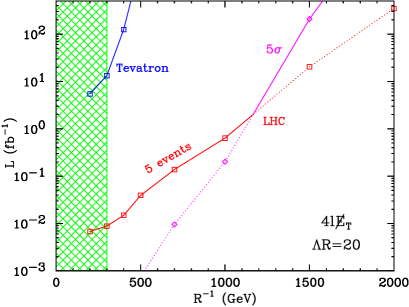
Figure 4: Discovery reach for the minimal $N=1$ UED model at the Tevatron (blue) and the LHC (red) in the $4\ell+\not\!\!E_{T}$ channel. The plot shows the total integrated luminosity per experiment, which is required for a $5\sigma$ discovery, given the observation of at least 5 events. Figure taken from Ref. [2].

From Fig. 2(b) one can notice that due to the presence of additional KK particles (spinless adjoints) at each level, the cascade decays become longer and may yield events with even more leptons. Such events with very high lepton multiplicity would be a smoking gun for the $N=2$ UED model [18].

3 Warped extra dimensions

The UED models discussed in the previous section are very peculiar: the extra dimension is an interval with a flat background geometry, and KK parity is realized as a geometric reflection about the midpoint of the extra dimension. It is important to note that KK parity has a larger parent symmetry, KK number conservation, which is broken only by the interactions living on the orbifold boundary points (the blue dots in Fig. 1). In the literature on UED models, it is usually assumed that the boundary interactions are symmetric with respect to the $Z_{2}$ reflection about the midpoint, so that KK parity is an exact symmetry. It is also assumed that they are suppressed (loop-induced), implying that KK number is still an approximate symmetry. These assumptions have very important phenomenological implications, as both KK parity and the approximate KK number conservation are needed to evade precision electroweak constraints for UED models. KK parity eliminates couplings of a single odd KK mode with the SM fields, whereas the approximate KK number conservation suppresses certain interactions among the even level KK modes, such as single coupling of the second KK mode with the SM, which are not forbidden by KK parity. In the end, both the odd and even KK modes are allowed to have masses well below 1 TeV. If there were only KK parity and not the approximate KK number conservation, experimental constraints would have required the second KK mass to be higher than 2 - 3 TeV and, therefore, the compactification scale to be around 1 TeV or higher (recall that in flat geometry KK modes are evenly spaced).

The flatness of wave function profiles in UED is not natural and reflects the fact that electroweak symmetry breaking is not addressed but just postulated. A model of dynamical symmetry breaking in UED would typically spoil the flatness of the Higgs profile and constraints on the KK scale would have to be reexamined accordingly. The virtue of UED is that mass scales of new particles are allowed to be very close to the electroweak scale at a few hundreds GeV, allowing for easy access at the LHC, and offering an interesting benchmark model for LHC searches. However, the UED model does not address the hierarchy between the Planck and the weak scale, nor does it address the fermion mass hierarchy. In contrast, as shown by Randall and Sundrum [21], warped extra dimensions have provided a new framework for addressing the hierarchy problem in extensions of the Standard Model.

3.1 Generic features of warped spacetime

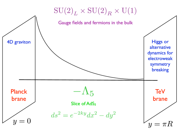
Figure 5: Randall–Sundrum set-up.

The Randall–Sundrum (RS) solution [21] is based on a slice of five-dimensional anti de Sitter space AdS₅ bounded by two three-branes, the UV and IR branes. The background space time metric of AdS₅ is

$$ds^{2}=e^{-2ky}\eta_{\mu\nu}dx^{\mu}dx^{\nu}-dy^{2}\,,$$ (1)

where $k$ is the AdS curvature scale of order the Planck scale (fixed by the bulk cosmological constant). The $y$ dependence in the metric is known as the “warp” factor. The UV (IR) brane is located at $y=0$ ($y=\pi R$) (see Fig. 5). The key point is that distance scales are measured with the nonfactorisable metric of AdS space. Hence, energy scales are location dependent along the fifth dimension and the hierarchy problem can be redshifted away. The RS model supposes that all fundamental mass parameters are of order the Planck scale. Owing to the warped geometry, the 4D (or zero-mode) graviton is localized near the UV/Planck brane, whereas the Higgs sector can be localized near the IR brane where the cut-off scale is scaled down to $M_{\tiny{Planck}}e^{-\pi kR}$. According to the AdS/CFT correspondence [22, 23], AdS₅ is dual to a 4D strongly-coupled conformal field theory (CFT). Thus, the RS solution is conjectured to be dual to composite Higgs models [24, 25, 26] where the TeV scale is hierarchically smaller and stable compared to the UV scale.

In the original RS model, the entire SM was assumed to be localized on the TeV brane. It was subsequently realized that when the SM fermion [27, 28] and gauge fields [29, 30, 31] are allowed to propagate in the bulk, such a framework not only solves the Planck-weak hierarchy, but can also address the flavor hierarchy. The idea is that light SM fermions (which are zero-modes of 5D fermions) can be localized near the UV brane, whereas the top quark is localized near the IR brane, resulting in small and large couplings respectively to the SM Higgs localized near the IR brane. In the CFT language, the Standard Model fermions and gauge bosons are partly composite to varying degrees, ranging from an elementary electron to a composite top quark. Finally, a central requirement in these constructions is having an approximate “custodial isospin” symmetry of the strong sector to protect the EW $\rho$ parameter. This is ensured by extending the EW gauge group to $SU(2)_{L}\times SU(2)_{R}\times U(1)$ [32].

In the RS setup, the KK modes are generically localized towards the IR brane. On the other hand, the zero mode gauge bosons have a flat profile along the extra dimension while the zero mode fermions can be arbitrarily localized in the bulk. An important resulting consequence for collider searches is that light fermions have small couplings to KK modes (including the graviton) while the top quark and the Higgs have a large coupling to KK modes.

3.2 Mass spectrum

The challenging aspect of RS collider phenomenology is that the mass scale of KK gauge bosons is constrained to be at least a few TeV by the electroweak and flavor precision tests. This is in part due to the absence of a parity symmetry (analogous to $R$-parity in SUSY or KK parity in UED), allowing tree-level exchanges to contribute to the precision observables. Nevertheless, in contrast with UED, there is not necessarily a single KK scale and some KK fermions are allowed to have a mass significantly different from KK gauge bosons. Indeed, the mass spectrum of KK fermions depends strongly on the type of boundary conditions (BC) imposed at the UV and IR branes as well as on the bulk mass parameter, called $c$ in Planck mass units. The $c$ parameter also fixes the localization of the wave function of the zero modes and therefore the mass of the SM fermion. As first emphasized in [33, 34], there can be very light KK fermions as a consequence of the top compositeness. BC are commonly modelled by either Neumann ($+$) or Dirichlet ($-$) BC in orbifold compactifications. Five-dimensional fermions lead to two chiral fermions in 4D, only one of which gets a zero mode to reproduce the chiral Standard Model fermion. SM fermions are associated with ($++$) BC (first sign is for Planck brane, second for TeV brane). The other chirality is ($--$) and does not have a zero mode. In the particular case of the breaking of the grand unified gauge group (GUT) to the SM, fermionic GUT partners which do not have zero modes are assigned Dirichlet boundary conditions on the Planck brane, i.e. they have ($-+$) boundary conditions . When computing the KK spectrum of $(-+)$ fermions one finds that for $c<1/2$ the lightest KK fermion is lighter than the lightest KK gauge boson. For the particular case $c<-1/2$, the mass of this KK fermion is exponentially smaller than that of the gauge KK mode. Fig. 6 shows the mass of the lightest ($-+$) KK fermion as a function of $c$ and for different values of the KK gauge boson mass $M_{KK}$. There is an intuitive argument for the lightness of the KK fermion: for $c\ll 1/2$, the zero-mode of the fermion with $(++)$ boundary condition is localized near the TeV brane. Changing the boundary condition to $(-+)$ makes this “would-be” zero-mode massive, but since it is localized near the TeV brane, the effect of changing the boundary condition on the Planck brane is suppressed, resulting in a small mass for the would-be zero-mode.

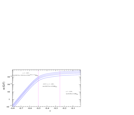
Figure 6: Mass of the (-+) KK fermion as a function of its $c$ parameter for different values of the KK gauge boson mass $M_{KK}=$3, 5, 7, 10 TeV (from bottom to top). For large and negative $c$, the KK fermion can be infinitely light.

Therefore, the scale for KK fermions can be different from the scale of KK gauge bosons. The lightest KK fermion is the one with the smallest $c$ parameter. For example, in the warped SO(10) models of Ref. [33, 34], the lightest KK fermion will come from the GUT multiplet which contains the top quark. Indeed, the top quark, being the heaviest SM fermion, is the closest to the TeV brane. This is achieved by requiring a negative $c$. Thus, all $(-+)$ KK fermions in the GUT multiplet containing the SM top quark are potentially light. Mass splittings between KK GUT partners of the top quark can have various origins, in particular due to GUT breaking in the bulk [33, 34]. Direct production at the LHC of light KK quarks leading to multi $W$ final states was studied in [36, 37].

3.3 Collider signals

As a result of wave function localization, SM gauge bosons and light fermions couple weakly to the KK states, whereas the KK states mostly decay to top quarks and longitudinal $W/Z$/Higgs. Hence, the golden decay channels such as resonant signals of dileptons or diphotons are suppressed. Besides, given that the KK mass scale is typically high (a few TeV) the top quarks or $W$ or $Z$ bosons resulting from the decays of these KK states are highly boosted.

The most widely studied particle is the KK gluon [38, 39, 40, 41, 42, 43, 44] which has the largest cross-section due to the QCD coupling and decays to jet final states. It was found that the LHC reach can be $\sim 4$ TeV, using techniques designed specifically to identify highly boosted top quarks.

Another central prediction of the RS model are the TeV Kaluza-Klein gravitons which have 1/TeV strength couplings since their wavefunctions are peaked near the TeV brane. They lead to distinct spin-2 resonances spaced according to the roots of the first Bessel function [45]. Signals from their direct production were investigated in [46].

Finally, an additional ingredient of RS phenomenology is the radion, the scalar mode of the 5D gravitational fluctuations, parameterizing the vibration mode of the inter-brane proper distance. Its mass is essentially a free parameter (it depends on the mechanism responsible for the stabilization of the inter-brane distance) but it is expected to be much lighter than the KK excitations [47]. Given that its couplings are suppressed by the warped-down Planck scale, the radion has observable effects at high energy colliders [47, 48, 49, 50, 51, 52]. Like the Higgs, the radion is located near the IR brane and its interactions are proportional to the mass of the field it couples to (through the trace of the energy-momentum tensor). The Higgs and radion can mix through a gravitational kinetic mixing term [53] with interesting consequences [47, 48, 49, 50, 51]. Signals from direct production of the radion have been studied in [54, 52, 55].

In addition to the searches for the radion, the KK graviton and the KK gluons, other studies of warped phenomenology at the LHC have dealt with KK neutral electroweak gauge bosons [56], KK (heavy) fermions [57]. All these signatures are common to RS models. Besides, new characteristic predictions appear in more specific models. We mentioned the light KK fermions which appear for instance in warped GUT models with $Z_{3}$ symmetry and LZP dark matter [33, 34] but more generically in models where the Higgs is a pseudo-Goldstone boson [26, 37]. They are for instance predicted in the gauge-Higgs unification models of Ref. [58] which contain a $Z_{2}$ mirror symmetry. The associated signatures are jets and missing energy and benefit from a large cross section (vector-like quarks are pair-produced via the standard QCD interactions). Other interesting warped models with distinctive phenomenologies have been proposed such as warped supersymmetric models [59]. A recent finding and a generic prediction of 5D models is the existence of stable skyrmion configurations [60] with phenomenological consequences that remain to be investigated.

4 SUSY-UED discrimination at the LHC

As discussed in Section 2.3, the generic collider signatures of the minimal UED models involve jets, leptons, and missing energy, just like the signatures of supersymmetry. In addition, the couplings of the KK partners are equal to those of their SM counterparts. The same property is shared by the superpartners in SUSY models. A natural question, therefore, is whether a given UED model can be experimentally differentiated from supersymmetry and vice versa. This issue is the subject of this section.

In general, there are two fundamental differences between UED and SUSY.

1. The spins of the SM particles and their KK partners are the same, while in SUSY they differ by $\frac{1}{2}$.

2. For each particle of the Standard Model, the UED models predict an infinite tower of new particles (Kaluza-Klein partners). In contrast, the simplest SUSY models contain only one partner per SM particle.

Thus the best way to discriminate between UED and SUSY is to either measure the spins of the new particles or to explore the higher level states of the KK tower.

Spin determinations in missing energy events are rather challenging (especially at hadron colliders), due to the presence of at least two invisible particles in each event, whose energies and momenta are not measured. Ideally, one would like to be able to reconstruct the energies and momenta of the escaping particles, in which case the spins can be determined in one of several ways (see Secs. 4.3, 4.4 and 4.5). However, when the momenta cannot be reliably determined, we are limited to studying only the properties of the particles which are visible in the detector, e.g. their invariant mass distributions (see Sec. 4.1).

On the other hand, it is relatively easier to find the higher KK modes, as long as they are produced abundantly. In particular, the $n=2$ excited KK states have positive KK parity and can directly decay into a pair of SM particles. Such higher level KK particles can then be looked for via traditional resonance searches (see Sec. 4.2). The observation of a rich resonance structure would be quite indicative of UED.

4.1 Spin measurements from invariant mass distributions

Consider the three-step decay chain exhibited in Fig. 7, which is rather typical in both UED and SUSY models. For example, in UED this chain may arise due to the $Q_{1}\to Z_{1}\to L_{1}\to\gamma_{1}$ transitions shown in Fig. 3. The measured visible decay products are a quark jet $j$ and two opposite sign leptons $\ell^{+}$ and $\ell^{-}$, while the end product $A$ is invisible in the detector. Given this limited amount of information, in principle there are 6 possible spin configurations for the heavy partners $D$, $C$, $B$ and $A$: $SFSF$, $FSFS$, $FSFV$, $FVFS$, $FVFV$, and $SFVF$, where $S$ stands for a spin-0 scalar, $F$ stands for a spin-$\frac{1}{2}$ fermion, and $V$ stands for a spin-1 vector particle. The main goal of the invariant mass analysis here will be to discriminate among these 6 possibilities, and in particular between $SFSF$ (SUSY) and $FVFV$ (minimal UED).

1.5 1.0   

Figure 7: The typical UED or SUSY cascade decay chain under consideration. At each vertex we assume the most general fermion couplings (see Ref. [61] for the exact definitions).

It is well known that the invariant mass distributions of the visible particles (the jet and two leptons in our case) already contain some information about the spins of the intermediate heavy particles $A$, $B$, $C$ and $D$ [62, 63, 64, 65]. Unfortunately, the invariant mass distributions are also affected by a number of additional factors, which have nothing to do with spins, such as: the chirality of the couplings at each vertex [66, 61]; the fraction of events $f$ in which the cascade is initiated by a particle $D$ rather than its antiparticle $\bar{D}$ [62]; and finally, the mass splittings among the heavy partners [63]. Therefore, in order to do a pure and model-independent spin measurement, one has to somehow eliminate the effect of those three extraneous factors.

Fortunately, the masses of $A$, $B$, $C$ and $D$ can be completely determined ahead of time, for example by measuring the kinematic endpoints of various invariant mass distributions made out of the visible decay products in the decay chain of Fig. 7 [67, 68, 69, 70], or through a sufficient number of transverse mass measurements [71, 72]. Once the mass spectrum is thus determined, we are still left with a complete lack of knowledge regarding the coupling chiralities and particle fraction $f$. In spite of this residual ambiguity, the spins can nevertheless be determined, at least as a matter of principle [61]. To this end, one should not make any a priori assumptions and instead consider the most general fermion couplings at each vertex in Fig. 7 and any allowed value for the parameter $f$. Then, the invariant mass distributions should be used to make separate independent measurements of the spins, on one hand, and of the couplings and $f$ fraction, on the other. Following the analysis of [61], here we shall illustrate this procedure with two examples — one from supersymmetry and one from UED. The corresponding mass spectra, chirality parameters and particle-antiparticle fraction $f$ for each case are listed in Table 1.

SPS1a UED500 $(m_{A},m_{B},m_{C},m_{D})$ in GeV (96, 143, 177, 537) (501, 515, 536, 598) $(f,\bar{f})$ (0.7, 0.3) (0.66, 0.34) $(a_{L},a_{R},b_{L},b_{R},c_{L},c_{R})$ (0, 1, 0, 1, 1, 0) (1, 0, 1, 0, 1, 0)

Table 1: Two study points from SUSY (SPS1a) and UED (UED500), characterized by particle masses, chirality coefficients and particle-antiparticle fractions $f$ and $\bar{f}$.

Given the three visible particles from the decay chain of Fig. 7, one can form three well-defined two-particle invariant mass distributions: one dilepton ($\ell^{+}\ell^{-}$), and two jet-lepton ($j\ell^{+}$ and $j\ell^{-}$) distributions. For the purposes of the spin analysis, it is actually more convenient to consider the sum and the difference of the two jet-lepton distributions [61]. The shapes of the resulting invariant mass distributions are given schematically by the following formulas [61]:

$$\left(\frac{dN}{dm^{2}_{\ell\ell}}\right)_{S} = F_{S;\delta}^{(\ell\ell)}(m^{2}_{\ell\ell})+\alpha\,F_{S;\alpha}^{(\ell\ell)}(m^{2}_{\ell\ell})$$ (2)

$$\left(\frac{dN}{dm^{2}_{j\ell^{+}}}\right)_{S}+\left(\frac{dN}{dm^{2}_{j\ell^{-}}}\right)_{S} = F_{S;\delta}^{(j\ell)}(m_{j\ell}^{2})+\alpha\,F_{S;\alpha}^{(j\ell)}(m_{j\ell}^{2})$$ (3)

$$\left(\frac{dN}{dm^{2}_{j\ell^{+}}}\right)_{S}-\left(\frac{dN}{dm^{2}_{j\ell^{-}}}\right)_{S} = \beta\,F_{S;\beta}^{(j\ell)}(m_{j\ell}^{2})+\gamma\,F_{S;\gamma}^{(j\ell)}(m_{j\ell}^{2})\ ,$$ (4)

where the functions $F$, given explicitly in [61], are known functions of the masses of particles $A$, $B$, $C$ and $D$. As indicated by the index $S$, there is a separate set of $F$ functions for each spin configuration: $S=\{SFSF,FSFS,\\ FSFV,FVFS,FVFV,SFVF\}\,.$ Thus the functions $F$ contain the pure spin information. On the other hand, the coefficients $\alpha$, $\beta$ and $\gamma$ encode all of the residual model dependence, namely the effect of the coupling chiralities and particle-antiparticle fraction $f$. Since the coefficients $\alpha$, $\beta$ and $\gamma$ are a priori unknown, they will need to be determined from experiment, by fitting the predicted shapes (2-4) to the data. The results from this exercise for the two study points from Table 1 are shown in Fig. 8. The solid (magenta) lines in each panel represent the input invariant mass distributions which will be presumably measured by experiment. The other (dotted or dashed) lines are the best fits to this data, for each of the remaining 5 spin configurations $S$. The color code is the following. A dashed (green) line indicates that the trial model fits the input data perfectly, while a dotted line implies that the fit fails to match the input data. The best fit values for the relevant coefficients ($\alpha$, $\beta$ and $\gamma$) for each case are also shown, except for those cases (labeled by “NA”) where they are left undetermined by the fit. Dotted lines of the same color imply that they are identical to each other, yet different from the input “data”.

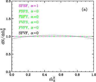
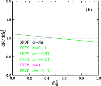
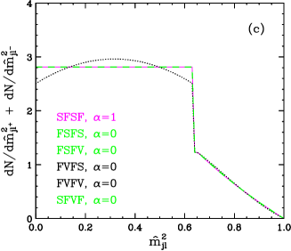
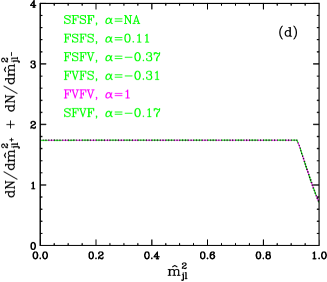
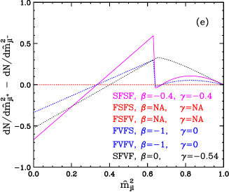
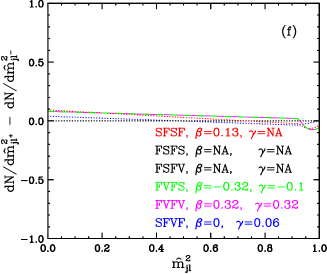
Figure 8: Best fits to the three invariant mass distributions predicted for the SUSY (a,c,e) and UED (b,d,f) study points from Table 1. The solid (magenta) line in each plot represents the input “data” while the other (dotted or dashed) lines are the best fits to the data for each of the remaining 5 spin configurations. Dashed green lines indicate a perfect match to the data, while dotted lines of any other color imply that the best fit fails to perfectly reproduce the data. The best fit values for the relevant coefficients ($\alpha$, $\beta$ and $\gamma$) are also shown.

The results from Fig. 8 show that the success of the spin measurement method depends on the type of new physics which happens to be discovered. In the case of supersymmetry (panels a,c,e), the spin chain can be unambiguously determined to be $SFSF$. Furthermore, this can be done solely on the basis of the distribution (4), which is sufficiently powerful to rule out all of the remaining 5 spin chain candidates. On the other hand, the UED case (panels b,d,f) is more challenging, and the end result is inconclusive — both models $FVFS$ and $FVFV$ are able to perfectly fit all three distributions (2-4). This confusion is not related to the specific choice of our UED study point, but is in fact a general feature of any $FVFV$ and $FVFS$ (as well as $FSFV$ and $FSFS$) pair of models [61]. In summary, it appears that through studies of the shapes of the invariant mass distributions of the visible decay products in a chain such as the one in Fig 7, one should be able to discriminate between SUSY and UED, while the specific type of UED model may remain uncertain.

4.2 Higher level KK resonance searches

As already mentioned earlier, the discovery of the higher level KK resonances would be another strong indication of the UED scenario. At hadron colliders like the LHC, resonance searches are easiest in the dilepton (dimuon or dielectron) channels. The corresponding 5$\sigma$ discovery reach for (a) $\gamma_{2}$ and (b) $Z_{2}$ is shown in Fig. 9 [17]. In each plot, the upper set of lines labeled “DY” makes use of the single $\gamma_{2}$ or $Z_{2}$ production only, while the lower set of lines (labeled “all processes”) includes in addition indirect $\gamma_{2}$ and $Z_{2}$ production from $n=2$ KK quark decays. The red dotted line marked “FNAL” in the upper left corner of (a) reflects the expectations for a $\gamma_{2}\to e^{+}e^{-}$ discovery at the Tevatron in Run II.

   

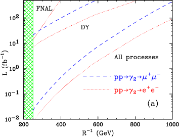
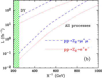
Figure 9: Total integrated luminosity needed for a 5$\sigma$ discovery of (a) $\gamma_{2}$ and (b) $Z_{2}$ as a dielectron (red) or dimuon (blue) resonance. The shaded area below $R^{-1}$ = 250 GeV indicates the region disfavored by precision electroweak data. Figures taken from Ref. [17].

While the discovery of an $n=2$ KK gauge bosons would be a strong argument in favor of UED, any such resonance by itself is not a sufficient proof, since it resembles an ordinary $Z^{\prime}$ gauge boson in supersymmetry. An important corroborating evidence in favor of UED would be the simultaneous discovery of several, rather degenerate KK gauge boson resonances, for which there would be no good motivation in generic SUSY models. The crucial question therefore is whether one can resolve the different $n=2$ KK gauge bosons as individual resonances. For this purpose, one would need to see a double peak structure in the invariant mass distributions, as illustrated in Fig. 10. We see that the diresonance structure is easier to detect in the dielectron channel, due to the better mass resolution. In dimuons, with L = 100 fb^-1 the structure is also beginning to emerge. We should note that initially the two resonances will not be separately distinguishable, and each will in principle contribute to the discovery of a broad bump. In this sense, the reach plots in Fig. 9 are rather conservative, since they do not combine the two signals from $Z_{2}$ and $\gamma_{2}$, but show the reach for each resonance separately.

   

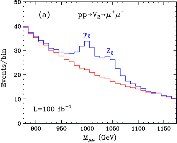
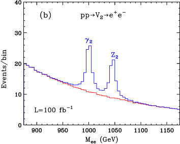
Figure 10: The $V_{2}\equiv\gamma_{2},Z_{2}$ diresonance structure in UED with $R^{-1}$= 500 GeV, for the (a) dimuon and (b) dielectron channel at the LHC with L = 100 fb^-1. The SM background is shown with the (red) continuous underlying histogram. Figures taken from Ref. [17].

4.3 Spin measurements from production cross-sections

The spin of the new particles can also be inferred from the threshold behavior of their production cross-section [11, 8]. For an $s$-channel diagram mediated by a gauge boson, the pair production cross-section for a spin-0 particle behaves like $\sigma\sim\beta^{3}$ while the cross-section for a spin-$\frac{1}{2}$ particle behaves as $\sigma\sim\beta$, where $\beta=\sqrt{1-\frac{4m^{2}}{s}}$, and $\sqrt{s}$ is the total center-of-mass energy, while $m$ is the mass of the new particle. At lepton colliders the threshold behavior can be easily studied by varying the beam energy and measuring the corresponding total cross-section, without any need for reconstructing the kinematics of the missing particles. In contrast, at hadron colliders the initial state partons cannot be controlled, so in order to apply this method, one has to fully reconstruct the final state, which is rather difficult when there are two or more missing particles.

The total production cross-section may also be used as an indicator of spin [73, 74]. For example, the total cross-sections of the fermion KK modes in UED are 5-10 times larger than the corresponding cross-sections for scalar superpartners of the same mass. However, the measurement of the total cross-section necessarily involves additional model-dependent assumptions regarding the branching fractions, the production mechanism, etc.

4.4 Spin measurements from angular distributions

Perhaps the most direct indication of the spin of the new particles is provided by the azimuthal angular distribution at production [11, 8]. Assuming production through an $s$-channel gauge boson, the angular distribution for a spin-0 particle is $\sim(1-\cos^{2}\theta)$, where $\theta$ is the azimuthal production angle in the center-of-mass frame. In contrast, the distribution for a spin-$\frac{1}{2}$ particle is $\sim(1+\cos^{2}\theta)$. Unfortunately, reconstructing the angle $\theta$ generally requires a good knowledge of the momentum of the missing particles, which is only possible at a lepton collider. Applying similar ideas at the LHC, one finds that typically quite large luminosities are needed [75].

4.5 Spin measurements from quantum interference

When a particle is involved in both the production and the decay, its spin $s$ can also be inferred from the angle $\phi$ between the production and decay planes [76, 77, 78]. The cross section can be written as

$$\frac{d\sigma}{d\cos\phi}=a_{0}+a_{1}\cos\phi+a_{2}\cos 2\phi+\cdots+a_{2s}\cos 2s\phi\ .$$ (5)

By measuring the coefficient $a_{2s}$ of the highest $\cos$ mode, one can in principle extract the spin $s$ of the particle. This method is especially useful since it does not rely on the particular production mechanism, and is equally applicable to $s$-channel and $t$-channel processes. However, its drawback is that the $\phi$ dependence results from integrating out all other degrees of freedom, which often leads to a vanishing coefficient as a result of cancellations, for instance, in the case of a purely vector-like coupling, or in the case of a $pp$ collider like the LHC. As a result, the practical applicability of the method is rather model-dependent.

Acknowledgements

KK is supported in part by the DOE under contract DE-AC02-76SF00515 and DE-AC02-07CH11359. KM is supported in part by a US Department of Energy grant DE-FG02-97ER41029. The work of GS is supported by the European Research Council.

References

- [1] T. Appelquist, H. C. Cheng and B. A. Dobrescu, “Bounds on universal extra dimensions,” Phys. Rev. D 64, 035002 (2001) [arXiv:hep-ph/0012100].
- [2] H. C. Cheng, K. T. Matchev and M. Schmaltz, “Bosonic supersymmetry? Getting fooled at the LHC,” Phys. Rev. D 66, 056006 (2002) [arXiv:hep-ph/0205314].
- [3] B. A. Dobrescu and E. Pontón, “Chiral compactification on a square,” JHEP 0403, 071 (2004) [arXiv:hep-th/0401032].
- [4] H. C. Cheng, K. T. Matchev and M. Schmaltz, “Radiative corrections to Kaluza-Klein masses,” Phys. Rev. D 66, 036005 (2002) [arXiv:hep-ph/0204342].
- [5] T. Flacke, A. Menon and D. J. Phalen, “Non-minimal universal extra dimensions,” Phys. Rev. D 79, 056009 (2009) [arXiv:0811.1598 [hep-ph]].
- [6] G. Burdman, B. A. Dobrescu and E. Ponton, “Resonances from two universal extra dimensions,” Phys. Rev. D 74, 075008 (2006) [arXiv:hep-ph/0601186].
- [7] E. Ponton and L. Wang, “Radiative effects on the chiral square,” JHEP 0611, 018 (2006) [arXiv:hep-ph/0512304].
- [8] M. Battaglia, A. Datta, A. De Roeck, K. Kong and K. T. Matchev, “Contrasting supersymmetry and universal extra dimensions at the CLIC multi-TeV e+ e- collider,” JHEP 0507, 033 (2005) [arXiv:hep-ph/0502041].
- [9] B. Bhattacherjee and A. Kundu, “The International Linear Collider as a Kaluza-Klein factory,” Phys. Lett. B 627, 137 (2005) [arXiv:hep-ph/0508170].
- [10] S. Riemann, “Z’ signals from Kaluza-Klein dark matter,” In the Proceedings of 2005 International Linear Collider Workshop (LCWS 2005), Stanford, California, 18-22 Mar 2005, pp 0303 [arXiv:hep-ph/0508136].
- [11] M. Battaglia, A. K. Datta, A. De Roeck, K. Kong and K. T. Matchev, “Contrasting supersymmetry and universal extra dimensions at colliders,” In the Proceedings of 2005 International Linear Collider Workshop (LCWS 2005), Stanford, California, 18-22 Mar 2005, pp 0302 [arXiv:hep-ph/0507284].
- [12] A. Freitas and K. Kong, “Two universal extra dimensions and spinless photons at the ILC,” JHEP 0802, 068 (2008) [arXiv:0711.4124 [hep-ph]].
- [13] K. Ghosh, “Probing two Universal Extra Dimension model with leptons and photons at the LHC and ILC,” JHEP 0904, 049 (2009) [arXiv:0809.1827 [hep-ph]].
- [14] K. Ghosh and A. Datta, “Probing two Universal Extra Dimensions at International Linear Collider,” Phys. Lett. B 665, 369 (2008) [arXiv:0802.2162 [hep-ph]].
- [15] T. G. Rizzo, “Probes of universal extra dimensions at colliders,” Phys. Rev. D 64, 095010 (2001) [arXiv:hep-ph/0106336].
- [16] C. Macesanu, C. D. McMullen and S. Nandi, “Collider implications of universal extra dimensions,” Phys. Rev. D 66, 015009 (2002) [arXiv:hep-ph/0201300].
- [17] A. Datta, K. Kong and K. T. Matchev, “Discrimination of supersymmetry and universal extra dimensions at hadron colliders,” Phys. Rev. D 72, 096006 (2005) [Erratum-ibid. D 72, 119901 (2005)] [arXiv:hep-ph/0509246].
- [18] B. A. Dobrescu, K. Kong and R. Mahbubani, “Leptons and photons at the LHC: Cascades through spinless adjoints,” JHEP 0707, 006 (2007) [arXiv:hep-ph/0703231].
- [19] K. Ghosh and A. Datta, “Phenomenology of spinless adjoints in two Universal Extra Dimensions,” Nucl. Phys. B 800, 109 (2008) [arXiv:0801.0943 [hep-ph]].
- [20] C. Lin, “A Search for universal extra dimensions in the multi-lepton channel from collisions at = 1.8 TeV,” FERMILAB-THESIS-2005-69.
- [21] L. Randall and R. Sundrum, “A large mass hierarchy from a small extra dimension,” Phys. Rev. Lett. 83, 3370 (1999) [arXiv:hep-ph/9905221].
- [22] J. M. Maldacena, “The large N limit of superconformal field theories and supergravity,” Adv. Theor. Math. Phys. 2, 231 (1998) [Int. J. Theor. Phys. 38, 1113 (1999)] [arXiv:hep-th/9711200].
- [23] E. Witten, “Anti-de Sitter space and holography,” Adv. Theor. Math. Phys. 2, 253 (1998) [arXiv:hep-th/9802150].
- [24] N. Arkani-Hamed, M. Porrati and L. Randall, “Holography and phenomenology,” JHEP 0108, 017 (2001) [arXiv:hep-th/0012148].
- [25] R. Rattazzi and A. Zaffaroni, “Comments on the holographic picture of the Randall-Sundrum model,” JHEP 0104, 021 (2001) [arXiv:hep-th/0012248].
- [26] R. Contino, Y. Nomura and A. Pomarol, “Higgs as a holographic pseudo-Goldstone boson,” Nucl. Phys. B 671, 148 (2003) [arXiv:hep-ph/0306259].
- [27] Y. Grossman and M. Neubert, “Neutrino masses and mixings in non-factorizable geometry,” Phys. Lett. B 474, 361 (2000) [arXiv:hep-ph/9912408].
- [28] T. Gherghetta and A. Pomarol, “Bulk fields and supersymmetry in a slice of AdS,” Nucl. Phys. B 586, 141 (2000) [arXiv:hep-ph/0003129].
- [29] H. Davoudiasl, J. L. Hewett and T. G. Rizzo, “Bulk gauge fields in the Randall-Sundrum model,” Phys. Lett. B 473, 43 (2000) [arXiv:hep-ph/9911262].
- [30] A. Pomarol, “Gauge bosons in a five-dimensional theory with localized gravity,” Phys. Lett. B 486, 153 (2000) [arXiv:hep-ph/9911294].
- [31] S. Chang, J. Hisano, H. Nakano, N. Okada and M. Yamaguchi, “Bulk standard model in the Randall-Sundrum background,” Phys. Rev. D 62, 084025 (2000) [arXiv:hep-ph/9912498].
- [32] K. Agashe, A. Delgado, M. J. May and R. Sundrum, “RS1, custodial isospin and precision tests,” JHEP 0308, 050 (2003) [arXiv:hep-ph/0308036].
- [33] K. Agashe and G. Servant, “Warped unification, proton stability and dark matter,” Phys. Rev. Lett. 93, 231805 (2004) [arXiv:hep-ph/0403143].
- [34] K. Agashe and G. Servant, “Baryon number in warped GUTs: Model building and (dark matter related) phenomenology,” JCAP 0502, 002 (2005) [arXiv:hep-ph/0411254].
- [35] C. Csaki, C. Grojean, J. Hubisz, Y. Shirman and J. Terning, “Fermions on an interval: Quark and lepton masses without a Higgs,” Phys. Rev. D 70, 015012 (2004) [arXiv:hep-ph/0310355].
- [36] C. Dennis, M. Karagoz Unel, G. Servant and J. Tseng, “Multi-W events at LHC from a warped extra dimension with custodial symmetry,” arXiv:hep-ph/0701158.
- [37] R. Contino and G. Servant, “Discovering the top partners at the LHC using same-sign dilepton final states,” JHEP 0806, 026 (2008) [arXiv:0801.1679 [hep-ph]].
- [38] K. Agashe, A. Belyaev, T. Krupovnickas, G. Perez and J. Virzi, “LHC signals from warped extra dimensions,” Phys. Rev. D 77, 015003 (2008) [arXiv:hep-ph/0612015].
- [39] B. Lillie, L. Randall and L. T. Wang, “The Bulk RS KK-gluon at the LHC,” JHEP 0709, 074 (2007) [arXiv:hep-ph/0701166].
- [40] M. Guchait, F. Mahmoudi and K. Sridhar, “Tevatron constraint on the Kaluza-Klein gluon of the bulk Randall-Sundrum model,” JHEP 0705, 103 (2007) [arXiv:hep-ph/0703060].
- [41] B. Lillie, J. Shu and T. M. P. Tait, “Kaluza-Klein Gluons as a Diagnostic of Warped Models,” Phys. Rev. D 76, 115016 (2007) [arXiv:0706.3960 [hep-ph]].
- [42] A. Djouadi, G. Moreau and R. K. Singh, “Kaluza–Klein excitations of gauge bosons at the LHC,” Nucl. Phys. B 797, 1 (2008) [arXiv:0706.4191 [hep-ph]].
- [43] M. Guchait, F. Mahmoudi and K. Sridhar, “Associated production of a Kaluza-Klein excitation of a gluon with a t t(bar) pair at the LHC,” Phys. Lett. B 666, 347 (2008) [arXiv:0710.2234 [hep-ph]].
- [44] M. Carena, A. D. Medina, B. Panes, N. R. Shah and C. E. M. Wagner, “Collider Phenomenology of Gauge-Higgs Unification Scenarios in Warped Extra Dimensions,” Phys. Rev. D 77, 076003 (2008) [arXiv:0712.0095 [hep-ph]].
- [45] L. Randall and R. Sundrum, “An alternative to compactification,” Phys. Rev. Lett. 83, 4690 (1999) [arXiv:hep-th/9906064].
- [46] A. L. Fitzpatrick, J. Kaplan, L. Randall and L. T. Wang, “Searching for the Kaluza-Klein Graviton in Bulk RS Models,” JHEP 0709, 013 (2007) [arXiv:hep-ph/0701150].
- [47] C. Csaki, M. L. Graesser and G. D. Kribs, “Radion dynamics and electroweak physics,” Phys. Rev. D 63, 065002 (2001) [arXiv:hep-th/0008151].
- [48] J. L. Hewett and T. G. Rizzo, “Shifts in the properties of the Higgs boson from radion mixing,” JHEP 0308, 028 (2003) [arXiv:hep-ph/0202155].
- [49] D. Dominici, B. Grzadkowski, J. F. Gunion and M. Toharia, “The scalar sector of the Randall-Sundrum model,” Nucl. Phys. B 671, 243 (2003) [arXiv:hep-ph/0206192].
- [50] D. Dominici, B. Grzadkowski, J. F. Gunion and M. Toharia, “Higgs-boson interactions within the Randall-Sundrum model,” Acta Phys. Polon. B 33, 2507 (2002) [arXiv:hep-ph/0206197].
- [51] J. F. Gunion, M. Toharia and J. D. Wells, “Precision electroweak data and the mixed radion-Higgs sector of warped extra dimensions,” Phys. Lett. B 585, 295 (2004) [arXiv:hep-ph/0311219].
- [52] C. Csaki, J. Hubisz and S. J. Lee, “Radion phenomenology in realistic warped space models,” Phys. Rev. D 76, 125015 (2007) [arXiv:0705.3844 [hep-ph]].
- [53] G. F. Giudice, R. Rattazzi and J. D. Wells, “Graviscalars from higher-dimensional metrics and curvature-Higgs mixing,” Nucl. Phys. B 595, 250 (2001) [arXiv:hep-ph/0002178].
- [54] T. G. Rizzo, “Radion couplings to bulk fields in the Randall-Sundrum model,” JHEP 0206, 056 (2002) [arXiv:hep-ph/0205242].
- [55] M. Toharia, “Higgs-Radion Mixing with Enhanced Di-Photon Signal,” Phys. Rev. D 79, 015009 (2009) [arXiv:0809.5245 [hep-ph]].
- [56] K. Agashe et al., “LHC Signals for Warped Electroweak Neutral Gauge Bosons,” Phys. Rev. D 76, 115015 (2007) [arXiv:0709.0007 [hep-ph]].
- [57] H. Davoudiasl, T. G. Rizzo and A. Soni, “On Direct Verification of Warped Hierarchy-and-Flavor Models,” Phys. Rev. D 77, 036001 (2008) [arXiv:0710.2078 [hep-ph]].
- [58] G. Panico, E. Ponton, J. Santiago and M. Serone, “Dark Matter and Electroweak Symmetry Breaking in Models with Warped Extra Dimensions,” Phys. Rev. D 77, 115012 (2008) [arXiv:0801.1645 [hep-ph]].
- [59] Y. Nomura, “Supersymmetric unification in warped space,” arXiv:hep-ph/0410348.
- [60] A. Pomarol and A. Wulzer, “Stable skyrmions from extra dimensions,” JHEP 0803, 051 (2008) [arXiv:0712.3276 [hep-th]].
- [61] M. Burns, K. Kong, K. T. Matchev and M. Park, “A General Method for Model-Independent Measurements of Particle Spins, Couplings and Mixing Angles in Cascade Decays with Missing Energy at Hadron Colliders,” JHEP 0810, 081 (2008), arXiv:0808.2472 [hep-ph].
- [62] A. J. Barr, “Using lepton charge asymmetry to investigate the spin of supersymmetric particles at the LHC,” Phys. Lett. B 596, 205 (2004) [arXiv:hep-ph/0405052].
- [63] J. M. Smillie and B. R. Webber, “Distinguishing spins in supersymmetric and universal extra dimension models at the Large Hadron Collider,” JHEP 0510, 069 (2005) [arXiv:hep-ph/0507170].
- [64] C. Athanasiou, C. G. Lester, J. M. Smillie and B. R. Webber, “Distinguishing spins in decay chains at the Large Hadron Collider,” JHEP 0608, 055 (2006) [arXiv:hep-ph/0605286].
- [65] L. T. Wang and I. Yavin, “Spin Measurements in Cascade Decays at the LHC,” JHEP 0704, 032 (2007) [arXiv:hep-ph/0605296].
- [66] C. Kilic, L. T. Wang and I. Yavin, “On the Existence of Angular Correlations in Decays with Heavy Matter Partners,” JHEP 0705, 052 (2007) [arXiv:hep-ph/0703085].
- [67] I. Hinchliffe, F. E. Paige, M. D. Shapiro, J. Soderqvist and W. Yao, “Precision SUSY measurements at LHC,” Phys. Rev. D 55, 5520 (1997) [arXiv:hep-ph/9610544].
- [68] B. C. Allanach, C. G. Lester, M. A. Parker and B. R. Webber, “Measuring sparticle masses in non-universal string inspired models at the LHC,” JHEP 0009, 004 (2000) [arXiv:hep-ph/0007009].
- [69] B. K. Gjelsten, D. J. Miller and P. Osland, “Measurement of SUSY masses via cascade decays for SPS 1a,” JHEP 0412, 003 (2004) [arXiv:hep-ph/0410303].
- [70] B. K. Gjelsten, D. J. Miller and P. Osland, “Measurement of the gluino mass via cascade decays for SPS 1a,” JHEP 0506, 015 (2005) [arXiv:hep-ph/0501033].
- [71] C. G. Lester and D. J. Summers, “Measuring masses of semi-invisibly decaying particles pair produced at hadron colliders,” Phys. Lett. B 463, 99 (1999) [arXiv:hep-ph/9906349].
- [72] M. Burns, K. Kong, K. T. Matchev and M. Park, “Using Subsystem MT2 for Complete Mass Determinations in Decay Chains with Missing Energy at Hadron Colliders,” JHEP 0903, 143 (2009) [arXiv:0810.5576 [hep-ph]].
- [73] A. Datta, G. L. Kane and M. Toharia, “Is it SUSY?,” arXiv:hep-ph/0510204.
- [74] G. L. Kane, A. A. Petrov, J. Shao and L. T. Wang, “Initial determination of the spins of the gluino and squarks at LHC,” arXiv:0805.1397 [hep-ph].
- [75] A. J. Barr, “Measuring slepton spin at the LHC,” JHEP 0602, 042 (2006) [arXiv:hep-ph/0511115].
- [76] M. R. Buckley, S. Y. Choi, K. Mawatari and H. Murayama, “Determining Spin through Quantum Azimuthal-Angle Correlations,” Phys. Lett. B 672, 275 (2009) [arXiv:0811.3030 [hep-ph]].
- [77] M. R. Buckley, B. Heinemann, W. Klemm and H. Murayama, “Quantum Interference Effects Among Helicities at LEP-II and Tevatron,” Phys. Rev. D 77, 113017 (2008) [arXiv:0804.0476 [hep-ph]].
- [78] M. R. Buckley, H. Murayama, W. Klemm and V. Rentala, “Discriminating spin through quantum interference,” Phys. Rev. D 78, 014028 (2008) [arXiv:0711.0364 [hep-ph]].