Break-down of the single-active-electron approximation for one-photon ionization of the B $\bm{{}^{1}\Sigma_{u}^{+}}$ state of H₂ exposed to intense laser fields

Abstract

Ionization, excitation, and de-excitation to the ground state is studied theoretically for the first excited singlet state B ${}^{1}\Sigma_{u}^{+}$ of H₂ exposed to intense laser fields with photon energies in between about 3 eV and 13 eV. A parallel orientation of a linear polarized laser and the molecular axis is considered. Within the dipole and the fixed-nuclei approximations the time-dependent Schrödinger equation describing the electronic motion is solved in full dimensionality and compared to simpler models. A dramatic break-down of the single-active-electron approximation is found and explained to be due to the inadequate description of the final continuum states.

I Introduction

Recently, there has been an increased interest in the development of intense light sources with wavelengths shorter than the one of the titanium:sapphire lasers. This includes both high-harmonic sources and, especially, the free-electron lasers (FEL) gen:made71 . Although the primary goal is to achieve radiation in the x-ray regime, also the vacuum UV is of some practical interest. Interesting results have recently been achieved, e. g., at the free-electron laser FLASH in Hamburg sfa:rude08 ; sfa:rich09 ; sfm:jian09 ; sfa:zhu09 .

For a laser pulse with a photon frequency centered at $\omega$ and a peak electric field $F_{0}$ the Keldysh parameter $\gamma=\sqrt{I_{p}/U_{p}}$ sfa:keld65 with the ionization potential $I_{p}$ and the ponderomotive energy $U_{p}=\frac{{F_{0}}^{2}}{4\omega^{2}}$ is usually used as a (rough) criterion to distinguish the so-called multiphoton ($\gamma>1$) and tunneling ($\gamma<1$) regimes. With the large photon energies as they are available from FELs one is likely to remain in the multiphoton regime. Interesting questions in this context are whether at these photon energies even lowest-order perturbation theory (LOPT) may be sufficient to properly describe most ionization processes in such laser pulses and at which intensities non-perturbative behavior sets in. A natural candidate for investigating these questions is H₂, since its two electrons exposed to intense laser pulses can be treated perturbatively sfm:apal01 ; sfm:apal02 and non-perturbatively sfm:kawa00 ; sfm:awas05 ; sfm:awas06 ; sfm:pala06 ; sfm:vann08 ; sfm:vann09 within full dimensionality.

Despite the fact that electronically excited states have been found theoretically and experimentally to be populated by a non-negligible amount in intense laser pulses sfa:debo92 ; sfa:jone93 ; sfa:hert97 ; sfa:mull99 ; sfa:nubb08 ; sfm:awas08 ; sfm:mans09 , most theoretical studies on H₂ exposed to laser fields have concentrated on the ground state as initial state. However, the field-induced coupling to the typically much more closely spaced neighbor states may complicate the strong-field behavior of excited states. On the other hand, since higher photon fluxes require lower target densities, the novel intense light sources may allow for direct studies of electronically excited states similar as for ions. Such an investigation was, e. g., recently demonstrated for HeH⁺ dia:pede07 ; dia:dumi09 .

To the authors’ knowledge, the only theoretical studies of excited states of H₂ in intense laser fields were reported in sfm:saen02c in which their behavior in a (quasi)static field was investigated and in sfm:bart08 in which one-photon ionization of the B ${}^{1}\Sigma_{u}^{+}$ state was considered within a newly developed single-active-electron (SAE) approximation based on Koopmans’ picture. In fact, the latter work has motivated the present investigation. Thus the first electronically excited state B ${}^{1}\Sigma_{u}^{+}$ of H₂ exposed to intense laser fields is considered and the validity of the SAE approximation for this excited state is investigated. The H₂ molecule is treated in the fixed-nuclei approximation at $R\,=\,2.2998\,a_{0}\,$ with the field polarization being parallel to the internuclear axis. First, 8 eV photons were considered as in sfm:bart08 . Motivated by the found order of magnitude deviation between the present full two-electron calculation and the one in sfm:bart08 , a larger photon-energy range within the regime of one-photon ionization is considered, but only for the case of a single open channel, i. e., before the photon energy is sufficient to leave the H${}_{2}^{+}$ ion in an electronically excited state. It may be noted that some of the photon energies used in the calculations are already available with FELs gen:andr00 ; gen:yu03 .

After a brief description of the methods in Sec. II the results are presented and discussed in Sec. III. This includes a discussion of the results for a photon energy of 8 eV in Sec. III.1 and for variable photon energies in Sec. III.2. A simple model for explaining the failure of the SAE is given in Sec. III.3, followed by a conclusion in Sec. IV. Atomic units are used, if not stated otherwise.

II Method

Most results of this work have been obtained by a full-dimensional solution of the time-dependent Schrödinger equation (TDSE) describing the two electrons of H₂ exposed to an intense laser pulse with linear polarization. The molecular axis is assumed to be aligned parallel to the electric field of the laser. The semi-classical non-relativistic dipole approximation is adopted in which the laser field is described classically, while the molecular system is treated quantum mechanically. The shown results are obtained for fixed internuclear separations. The details of the approach have been given previously sfm:awas05 ; sfm:awas06 ; sfm:awas08 ; sfm:vann08 and are thus only briefly repeated.

The electronic TDSE describing H₂ in a laser field is given within the above-mentioned approximations as

$$\imath\frac{\partial}{\partial t}\Psi({\bf r}_{1},{\bf r}_{2},t)\,=\,\left(\hat{\rm H}_{0}\,+\,\hat{\rm D}(t)\right)\Psi({\bf r}_{1},{\bf r}_{2},t)\quad$$ (1)

where $\hat{\rm H}_{0}$ is the field-free electronic Hamiltonian of H₂ and $\hat{\rm D}(t)$ describes the interaction with the field. This interaction may be given in either velocity form, $\hat{\rm D}(t)={\bf A}(t)\cdot({\bf p}_{1}+{\bf p}_{2})$, or in length form, $\hat{\rm D}(t)=-{\bf F}(t)\cdot({\bf r}_{1}+{\bf r}_{2})$, where ${\bf p}_{i}$ is the momentum operator of electron $i$ while ${\bf A}$ and ${\bf F}$ represent vector potential and the electric field, respectively.

The wavefunction

$$\Psi({\bf r}_{1},{\bf r}_{2},t)\>=\>\sum_{nL}\>b_{nL}(t)\,\phi_{nL}({\bf r}_{1},{\bf r}_{2})$$ (2)

is expanded in terms of the field-free states $\phi_{nL}$ and the time-dependent coefficients $b_{nL}(t)$. The field-free wavefunctions $\phi_{nL}({\bf r}_{1},{\bf r}_{2})$ and corresponding energy eigenvalues $E_{nL}$ are obtained from the solution of the time-independent Schrödinger equation (TISE),

$$\hat{\rm H}_{0}\phi_{nL}({\bf r}_{1},{\bf r}_{2})\>=\>E_{nL}\phi_{nL}({\bf r}_{1},{\bf r}_{2})\quad.$$ (3)

A combined index $L$ is used for the specification of the symmetry. In this work it is limited to either ${}^{1}\Sigma_{g}$ ($L=0$) or ${}^{1}\Sigma_{u}$ ($L=1$) symmetry. The index $n=1,2,\dots$ just numbers the different states for a given symmetry $L$.

The field-free two-electron wavefunctions $\phi_{nL}$ are obtained by a configuration-interaction (CI) calculation performed in a basis of H${}_{2}^{+}$ orbitals. The H${}_{2}^{+}$ orbitals are expressed in a $B$-spline basis set in prolate-spheroidal coordinates. Since the basis functions are confined to a finite spatial volume, a discretized representation of the electronic continuum is obtained. Substitution of Eq. (2) into Eq. (1) yields then a finite set of coupled differential equations for the time-dependent coefficients $b_{nL}$. These equations are solved numerically with the initial condition $b_{nL}(t=0)\,=\,\delta_{n,1}\,\delta_{L,1}$ for the B ${}^{1}\Sigma_{u}^{+}$ state.

In the present work, the TISE for H${}_{2}^{+}$ is solved in a box of size 350 $a_{0}$. The solution of the TISE for H${}_{2}^{+}$ is obtained in prolate spheroidal coordinates ($1\,\leq\,\xi\,<\,\infty,-1\,\leq\,\eta\,\leq\,1,0\,\leq\,\phi\,<\,2\pi$). The total symmetry of the H${}_{2}^{+}$ states is defined on the basis of angular momentum and gerade or ungerade symmetry of the state wavefunction. For each total symmetry of H${}_{2}^{+}$ 350 $B$ splines of order 15 are used in $\xi$ direction and 24 $B$ splines of order 8 in $\eta$ direction. H${}_{2}^{+}$ states with angular momenta between 0 and 5 with gerade and ungerade symmetry are calculated. Using such a basis set yields around 4200 states for each total symmetry of H${}_{2}^{+}$. The CI calculation performed with these H${}_{2}^{+}$ states gives around 8000 states for each symmetry of H₂ (${}^{1}\Sigma_{g}^{+}$ and ${}^{1}\Sigma_{u}^{+}$).

For computational convenience, cos²-shaped pulses

$$X(t)\,=\,X_{0}\,\cos^{2}(\pi\,t/\tau)\,\cos(\omega\,t\,+\,\phi_{\rm CEP})$$ (4)

where $\omega$ is the photon energy and $X$ stands for $F$ (length form) or $A$ (velocity form) are used in most of the calculations of this work. (Note, the pulses defined this way are not identical for $X=F$ or $X=A$, especially in the case of extremely short pulses.) The peak electric field or vector potential amplitudes are $F_{0}$ and $A_{0}$, respectively. In order to obtain the maximum field at the center of the pulse, the carrier-envelope phase (CEP) $\phi_{\rm CEP}$ is set to 0 ($\pi/2$) for the length (velocity) form. The advantage of the cos² pulses is the finite pulse length $\tau$ (in the interval $[-\tau/2,\tau/2]$) and thus the well-defined interval for time integration. This is an evident advantage compared with the (more realistic) Gaussian pulse

$$X(t)\,=\,X_{0}\,\exp\left(-\frac{2\,t^{2}}{{\tau_{g}}^{2}}\right)\,\cos(\omega\,t\,+\,\phi_{\rm CEP})$$ (5)

that only exponentially decays to zero and requires thus a careful convergence study with respect to the integration interval. In order to assure that found deviations to the calculation in sfm:bart08 are not caused by a possible difference in the definition of the pulse shape, the results of cos² and Gaussian pulses are compared. In this case the characteristic time $\tau_{g}$ of the Gaussian pulse is chosen according to

$$\tau_{g}\,=\,\frac{\tau}{4}\,\sqrt{-\frac{1}{2}\ln\left(\frac{1}{2}\right)}\,\quad.$$ (6)

This choice yields the same full width at half maximum (FWHM) of the Gaussian and the cos² pulses.

For sufficiently low intensities one expects lowest-order perturbation theory (LOPT) to adequately describe the interaction of a molecule with a laser field. Within LOPT the $N$-photon ionization rate $\Gamma^{(N)}$ (in s^-1) is given by

$$\Gamma^{(N)}\,=\,\sigma^{(N)}\,\left(\frac{I}{\hbar\omega}\right)^{N}$$ (7)

where $I$ is the intensity of the monochromatic laser field in W/cm², $\hbar\omega$ is the photon energy in Joule, and $\sigma^{(N)}$ is the generalized $N$-photon ionization cross section in cm^2Ns^N-1. For single-photon ionization $\sigma^{(1)}$ is equal to the standard one-photon cross-section and LOPT reduces to Fermi’s Golden Rule. Integration of Eq. (7) over the intensity profile of a pulse gives the ionization yield

$$P_{\rm ion}^{\rm LOPT}\,=\,1-\exp\left(-\int_{\rm Pulse}\Gamma^{(N)}(I(t))\;dt\right)$$ (8)

where $\Gamma^{(N)}$ is a function of intensity $I$ (see Eq. (7)) which for a laser pulse is a function of time $t$. The generalized cross-sections $\sigma^{(N)}$ are in this work calculated with the same field-free two-electron states $\phi_{nL}$ of Eq. (3) that are used for solving the TDSE. Results within LOPT have been earlier obtained for H₂ in sfm:apal01 ; sfm:apal02 and a comparison to TDSE results was given in sfm:awas05 . In those references technical details on the evaluation of $\sigma^{(N)}$ may be found. However, in those previous investigations only ionization from the electronic ground state was considered.

For a more detailed investigation of the validity of the SAE approach introduced in sfm:bart08 it is of interest to consider also alternative SAE models. In one approach the TDSE is solved as discussed above, but a restricted set of configurations is used in the CI calculation. In this case only configurations are adopted in which one electron occupies the lowest lying ($1\,\sigma_{g}$) orbital of H${}_{2}^{+}$. The other electron may then occupy any of the $n\,\sigma_{g}$ ($n\,\sigma_{u}$) orbitals to yield the configurations for the CI calculation giving the ${}^{1}\Sigma_{g}$ (${}^{1}\Sigma_{u}$) states of H₂. This approach is referred to as pseudo SAE (p-SAE) sfa:lamb98a ; sfm:awas08 ; sfa:nubb08 . The p-SAE approach corresponds to a complete relaxation of the core. A frozen-core SAE approach where there is no relaxation of the core has recently been introduced in sfm:awas08 . In that case the core electrons are frozen in their field-free initial-state orbitals and the TDSE is solved for the active electron in the combined field of the core and the laser pulse. In the implementation the core was described within density-functional theory (DFT). For strong-field excitation and ionization of ground-state H₂ it was, however, demonstrated that the results agree quite well with the ones obtained with a core described within Hartree-Fock theory, despite the rather different electronic binding energies. The DFT-based variant used in this work will be referred to as DFT-SAE.

Two of the SAE approaches, p-SAE and DFT-SAE, give the ionization yield for a single electron. In sfm:awas08 it was found that for ionization yields of up to about 10 % the SAE results for H₂ should be multiplied by a factor 2 in order to properly account for the two equivalent electrons. However, for larger ion yields this factor 2 leads to an overestimation, because the screening of the core electron is reduced. As a consequence, the ionization potential increases and the ionization probability decreases. Therefore, the ion yield of the SAE approximation approaches the full CI-TDSE result for high intensities and ion yields larger than about 20 %. However, this screening argument applies in principle only, if the ionization process depends strongly on the electronic binding energy. This is, e. g., the case for ionization in the tunneling picture, but is not expected to be valid in the opposite extreme of perturbative single-photon ionization. It should be noted that no prefactor should be used in the Koopmans’-picture based SAE approach (K-SAE) of Barth et al. sfm:bart08 .

III Results

Table 1: State energies (in atomic units E_h) using different approaches at $R=2.2998$ a₀. The ionization potential of the B ${}^{1}\Sigma_{u}^{+}$ states is shown in the last column.

Approach	H2  X ${}^{1}\Sigma_{g}^{+}$	H2  B ${}^{1}\Sigma_{u}^{+}$	H2+  X ${}^{2}\Sigma_{g}$	Ip(B ${}^{1}\Sigma_{u}^{+}$)
CI	$-1.10374$	$-0.7485$	$-0.5989$	$0.1496$
p-SAE	$-1.06385$	$-0.7388$	$-0.5989$	$0.1399$
DFT-SAE	$-1.08196$	$-0.8381$	$-0.5989$	$0.2392$
K-SAE sfm:bart08	n. a.	$-0.7509$	$-0.5988$	$0.1521$
Accurate	$-1.1111725$ dia:kolo65	$-0.7563608186$ dia:woln88	$-0.5989$	$0.1575$

In Table 1 the energies of the ground (X ${}^{1}\Sigma_{g}^{+}$) and the first excited (B ${}^{1}\Sigma_{u}^{+}$) states of H₂ are given at the internuclear separation $R=2.2998$ a${}_{0}\,$. Furthermore, the corresponding ground-state energies of the H${}_{2}^{+}$ ion are shown together with the ionization potential of the B ${}^{1}\Sigma_{u}^{+}$ state that follows from them. The energies obtained by means of K-SAE (given in sfm:bart08 ), CI, p-SAE, and DFT-SAE approaches are compared. The best available theoretical energy values are also shown. While the energy of the B ${}^{1}\Sigma_{u}^{+}$ state obtained with K-SAE is in very good agreement with the CI calculation, the DFT-SAE result is almost 0.09 a.u. (2.4 eV) away. The p-SAE result is much closer to the CI result, but not as close as K-SAE. Since the ionic ground-state energies agree very well for all approaches, the differences found for the ionization potentials are a result of the different B ${}^{1}\Sigma_{u}^{+}$ energies. For completeness, also the different ground-state energies are given, if available. In this case, DFT-SAE agrees better to CI than p-SAE. It was demonstrated in dia:vann04 ; dia:vann06 that very accurate CI results can be obtained with the present approach, if the basis-set parameters including the configurations are judiciously chosen. However, for solving the TDSE a compromise has to be made, since a large spectrum of field-free states including the electronic continuum has to be described with reasonable accuracy.

The reason for the very poor DFT energy of the B ${}^{1}\Sigma_{u}^{+}$ state is probably twofold. First, small systems like He and H₂ are known to be difficult to be described by DFT. More importantly, however, standard DFT is in principle not applicable to excited states. In practice, time-dependent DFT is usually adopted to obtain excitation energies. Nevertheless, it should be interesting to investigate the performance of the recently developed DFT based SAE in comparison to the also very newly proposed K-SAE as is done below.

III.1 8 eV photons

In sfm:bart08 it was concluded that single-photon ionization of the B ${}^{1}\Sigma_{u}^{+}$ state of H₂ at 8 eV should satisfy the conditions for the applicability of a time-dependent extension of Koopmans’ picture, a single-active-electron approximation based on Koopmans’ theorem, i. e. within K-SAE. Therefore, the response to a 5-cycle laser pulse with 8 eV photons was studied in the framework of the newly developed K-SAE. The TDSE was solved on a grid using the length formulation. In sfm:bart08 the calculated ionization yield plotted against the laser peak intensity on a log-log scale showed a slope 1 in a large range of intensities. This confirmed the perturbative nature of the single-photon process in the selected intensity window and was interpreted as a further confirmation of the proper implementation of the time-propagation in the K-SAE approach. Note, in sfm:bart08 the laser peak intensity is defined as $I=\epsilon_{0}cF_{0}^{2}$ where $\epsilon_{0}$ is the vacuum permittivity, $c$ is the vacuum speed of light, and $F_{0}$ is the peak value of the electric field. In this work the alternative, cycle averaged peak intensity $I=\frac{1}{2}\epsilon_{0}cF_{0}^{2}$ is used.

Table 2: Comparison of K-SAE, CI, LOPT, p-SAE, and DFT-SAE results. The populations of the initial B ${}^{1}\Sigma_{u}^{+}$ state and the ionization yields are given for two different values of the peak electric field. The K-SAE results are taken from sfm:bart08 .

	F0 (a.u.)	K-SAE	CI	LOPT	p-SAE	DFT-SAE
Initial	0.005	n.a.	0.960	0.963	0.967	0.980
Ion.	0.005	0.0043	0.033	0.037	0.0031	0.022
Initial	0.020	0.930	0.548	0.543	0.624	0.728
Ion.	0.020	0.066	0.379	0.457	0.036	0.261

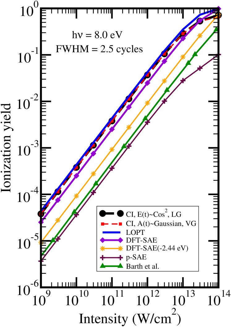
Figure 1: Ionization yield as a function of the peak laser intensity. The TDSE calculation is performed using length-form transition dipole moments with a $\cos^{2}$ envelope for the electric field (black, circles) and velocity-form transition dipole moments with a Gaussian envelope for the vector potential (red, squares). The FWHM for both pulses is $2.5\,$ cycles of $8\,$eV photon energy. The ionization yields obtained with LOPT (blue, solid line), DFT-SAE (violet, diamonds), scaled DFT-SAE by shifting the photon energy by $-2.44\,$eV (at 10.44 eV) (orange, asterix), and p-SAE (maroon, plus) are also shown and compared to the results from Barth et al. sfm:bart08 (green, triangles).

Besides the graphically shown intensity scan, the ionization yield and (in one case) the population remaining in the initial B ${}^{1}\Sigma_{u}^{+}$ state of H₂ were given in numerical form for the peak electric fields $F_{0}=0.005$ and $0.02\,$a. u. in sfm:bart08 . In Table 2 these results are compared to the corresponding values obtained in this work within the different approaches, CI-TDSE, LOPT, p-SAE, and DFT-SAE. In LOPT the initial-state population $P_{\rm ini}$ was defined as $P_{\rm ini}=1-P_{\rm ion}^{\rm LOPT}$.

The ionization yield predicted on the basis of K-SAE differs substantially from the CI-TDSE result. At the lower field strength ($F_{0}=0.005\,$a. u.) the K-SAE yield is almost one order of magnitude (factor 7.7) too small. For $F_{0}=0.02\,$a. u. the disagreement is a little bit smaller (factor 5.7). While p-SAE deviates from the CI-TDSE results even more than K-SAE (underestimation by factors 10.6 and 10.5), DFT-SAE appears on the first glance to be the SAE model with the best agreement to the full two-electron result, despite the poor energy of the B ${}^{1}\Sigma_{u}^{+}$ state. Although the DFT-SAE yields are also smaller than the CI-TDSE ones, they differ only by factors 1.5 and 1.45 for the smaller and the larger field strengths, respectively. Clearly the best agreement to the CI-TDSE result is, however, obtained with LOPT. At the lower field strength the agreement is in fact good (the CI-TDSE yield is overestimated by a factor 1.1 only) and for the larger field strength it is still reasonable (factor 1.2). Note, the given fields correspond to laser peak intensities of about $8.8\times 10^{11}\,$W/cm² and $1.4\times 10^{13}\,$W/cm² where LOPT is not necessarily expected to work. The one-photon cross-section at 8 eV is found to be $\sigma^{(1)}=5.75\times 10^{-17}\,$cm².

A Taylor expansion of the exponential in Eq. (8) and insertion of Eq. (7) shows that for one-photon ionization the ion yield is proportional to the one-photon absorption cross-section and the laser intensity, $P_{\rm ion}^{\rm LOPT}\propto\sigma^{(1)}\,I$, if the time integral is small. Therefore, one expects within LOPT and for small ion yields that an increase of the field strength by a factor 4 leads to an increase of the ion yield by a factor $4^{2}=16$. This factor is reproduced well for K-SAE (15.3), but neither for CI-TDSE (11.5) nor for LOPT (12.4). The latter result shows that for the larger ionization yields found for the two-electron models CI-TDSE and LOPT the assumption of a sufficiently small time integral is not fulfilled and the ion yield does not increase linearly with intensity, even within LOPT. Correcting the K-SAE yield at the larger field for this effect shows that the agreement between K-SAE and CI-TDSE does in fact not improve for the higher field, but the disagreement remains at a factor of about 7.5. While the factor 11.9 found between the two ion yields obtained with DFT-SAE appears understandable from the similar magnitude of ionization as compared with CI-TDSE and LOPT, one would expect for p-SAE a factor close to 16 similar to K-SAE, since the ion yield is even smaller. However, instead a value 11.6 is found, similar to the other cases except K-SAE.

The pronounced failure of K-SAE despite the very accurate energy of the B ${}^{1}\Sigma_{u}^{+}$ state is clearly surprising. In order to clarify this issue it was checked that it is not an artifact of the different numerical implementations. One possibility could, e. g., be a different pulse definition, or the use of the velocity or length forms of the dipole operator. In Fig. 1 the ionization yield as a function of the laser peak intensity is shown. It confirms the already discussed good agreement of CI-TDSE with LOPT. The ionization yield obtained by means of DFT-SAE is quite close to the full CI-TDSE results. The p-SAE and K-SAE fail by almost an order of magnitude for 8 eV photons. In order to investigate the sensitivity of the results on pulse details and the form of the dipole operator used, two CI-TDSE results are shown in Fig. 1. In one case a cos² pulse envelope (for $E(t)$) is used with dipole moments in length form, while in the other case a Gaussian pulse shape (for $A(t)$) is used together with the velocity form. Clearly, neither the choice of the dipole operator nor the exact pulse shape (in both cases a FWHM of 2.5 cycles is used) modifies the result substantially. In fact, the agreement is almost perfect, except for very high intensities and thus very close to saturation.

In view of the rather poor energy of the B ${}^{1}\Sigma_{u}^{+}$ state in DFT-SAE the superior result compared to the other SAE models is suspicious. In fact, as has been discussed previously in sfa:lamb00 ; sfm:apal02 ; sfm:awas05 a poor initial-state energy should be accounted for by a correspondingly shifted photon energy. This energy shift should be chosen in such a way that the correct multi-photon ionization threshold (in this case the one-photon threshold) is obtained. Since the present DFT threshold lies about 2.44 eV higher than the one of the CI calculation (see Table 1), the CI-TDSE results for a photon energy of 8 eV should be compared to the DFT-SAE results at a photon energy of 10.44 eV. The corresponding curve (also drawn in Fig. 1) shows that the agreement with CI-TDSE worsens evidently, although it remains better than the agreement of the other SAE models with the CI-TDSE result. It is clear, however, that the (slightly) better agreement of DFT-SAE appears to be accidental.

It is, of course, interesting to investigate the origin of the rather evident failures of K-SAE and p-SAE. A characteristic property of the B ${}^{1}\Sigma_{u}^{+}$ state of H₂ is its rather large ionic component dia:shar71 . In fact, it was shown theoretically that this ionic character plays a crucial role in the strong-field behaviour of H₂. For example, it is responsible for bond softening and enhanced ionization of neutral H₂ sfm:saen00a ; sfm:saen00b ; sfm:haru00 ; sfm:kawa00 ; sfm:saen02a . The field-induced admixture of the ionic (H⁺H^-) component to the X ${}^{1}\Sigma_{g}^{+}$ ground state leads to strongly enhanced ionization, since H^- possesses a very low electronic binding energy. It appears quite reasonable that SAE models fail to properly describe the ionic component of the B ${}^{1}\Sigma_{u}^{+}$ state, since the (frozen) spectator electron always occupies a molecular orbital that is symmetrically distributed over both protons. As already discussed, the lack of even a very small admixture of the ionic component may reduce the ionization rate in a strong electric field significantly. This could explain the too low ionization yield found uniformly for all SAE models discussed in this work.

However, the good agreement between LOPT and CI-TDSE (especially at low intensities) allows to conclude that one should not look for a strong-field explanation where the binding energy influences the ionization rate in an exponential way. Instead, the validity of the LOPT indicates that it is only the (direct) transition dipole matrix element between the initial B ${}^{1}\Sigma_{u}^{+}$ state and the continuum (reached with an 8 eV photon) that determines the magnitude of ionization. In fact, a rough estimate based on a simplified model describing ionization from such an ionic pair state (weighted by the contribution of this state to the B ${}^{1}\Sigma_{u}^{+}$ state of H₂) indicates that this ionic component cannot at all explain a massive increase of the one-photon ionization yield. Another possible explanation of the failure of a SAE model could be the occurrence of doubly-excited autoionizing states that are necessarily absent in SAE models. However, they are expected to be excited at photon energies larger than 8 eV dia:sanc97b ; dia:vann06 .

III.2 One-photon ionization

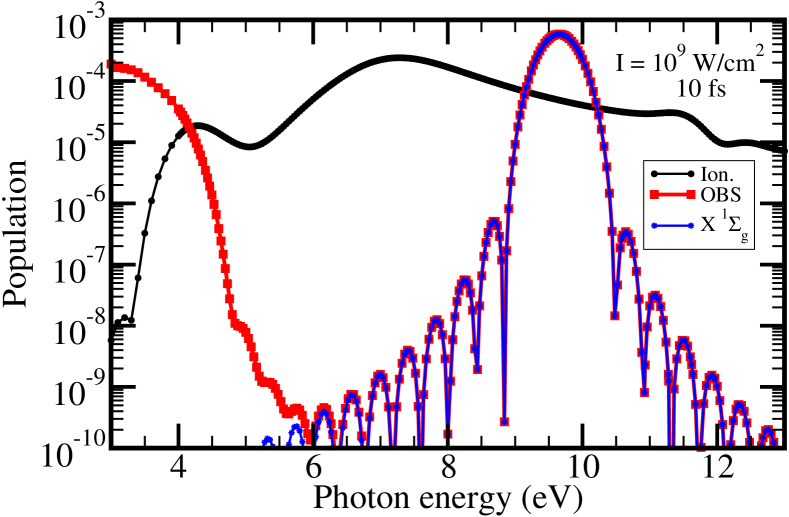
Figure 2: Ionization (black, circles), population of the other bound states OBS (red, dashed), and population of the X ${}^{1}\Sigma_{g}^{+}$ ground state (blue, asterix) obtained with CI-TDSE as a function of the incident photon energy for a $10\,$fs laser pulse with a peak intensity of $1.0\times 10^{9}\,$W/cm².

A more complete picture of one-photon ionization from the B ${}^{1}\Sigma_{u}^{+}$ state of H₂ may be obtained from a consideration of the photon-energy dependence. Figure 2 shows the ionization yield of the H₂ B ${}^{1}\Sigma_{u}^{+}$ state exposed to a $10\,$fs laser pulse with a peak intensity of $1.0\times 10^{9}\,$W/cm² obtained with CI-TDSE. The photon energy varies between about 3 and 13 eV and covers thus the one-photon regime from just below the ionization threshold to the energy at which the first excited electronic state of H${}_{2}^{+}$ becomes energetically accessible. Due to the finite pulse width (and possible two-photon ionization) the ionization starts before the threshold energy of about 4.1 eV. In contrast to one-photon ionization starting from the electronic ground state which shows an overall monotonous decrease with increasing photon energy dia:sanc97a , the ionization yield of the B ${}^{1}\Sigma_{u}^{+}$ state decreases until about 5 eV after which it increases drastically (note the logarithmic scale) until about 7 eV. Beyond about 7 eV the yield decreases monotonously, until some structure due to the occurrence of autoionizing states becomes visible in between about 11 eV and 12.5 eV. Clearly, the autoioinizing states cannot explain the failure of the SAE approaches at 8 eV discussed in Sec. III.1.

The population of the H₂ X ${}^{1}\Sigma_{g}^{+}$ ground state after the laser pulse is also shown in Figure 2. A pronounced maximum occurs at the expected energy of about 9.66 eV at which the B ${}^{1}\Sigma_{u}^{+}$ $\rightarrow$ X ${}^{1}\Sigma_{g}^{+}$ transition becomes resonant. The width of the peak reflects the spectral width of the laser pulse. For the considered laser peak intensity the population of the ground state and thus the probability for deexcitation of the B ${}^{1}\Sigma_{u}^{+}$ state is at its maximum about a factor 10 larger than the ionization yield. Since the total depopulation of the B ${}^{1}\Sigma_{u}^{+}$ state is, however, still very small (less than 0.1 %), the ionization probability remains practically uninfluenced by this deexcitation process. As was shown recently in sfm:vann08 , the oscillations (side peaks) of the resonant peak are due to the cos² shape of the pulse used in the calculation. Since they are many orders of magnitude smaller than the ionization yield, the latter is, however, not influenced by these spurious oscillations. This is also confirmed explicitly for 8 eV photons in Fig. 1, since the ion yields obtained with a Gaussian pulse that does not show these oscillations agrees well with the ones obtained with a cos² pulse.

The population of the other bound states (OBS) is also shown in Figure 2. It is defined as $P_{\rm OBS}=1-(P_{\rm ini}+P_{\rm ion})$ where $P_{\rm ini}$ is the population of the initial B ${}^{1}\Sigma_{u}^{+}$ state and $P_{\rm ion}$ is the ionization yield). In a large range of photon energies $P_{\rm OBS}$ is dominated by the ground-state contribution. Only below 6 eV the energetically higher lying bound states come into play. Close to the ionization threshold the ion yield and $P_{\rm OBS}$ cross each other. Below threshold the Rydberg states of H₂ are resonantly populated, while the one-photon ionization channel closes. As already mentioned, the finite band width of the adopted laser pulse leads to a rather broad energy range in which excitation and ionization compete with each other.

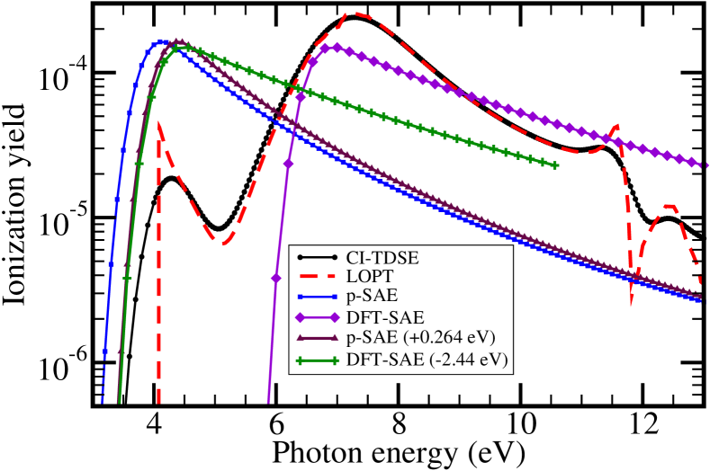
Figure 3: Photon-energy dependent ionization yield for various theoretical models with laser parameters as in Fig.  2. The ionization yields obtained with CI-TDSE (black, circles), LOPT(red, dashed), p-SAE (blue, square), and DFT-SAE (violet, diamonds) are compared. The ionization yields obtained by a shift of the photon energy to compensate the corresponding error in the ionization potential with respect to CI of p-SAE (maroon, triangles) and DFT-SAE (green, plus) are also shown.

Figure 3 shows the ionization yields obtained by means of the different theoretical models in the one-photon ionization regime. The laser parameters are the same as the ones in Figure 2. The ionization yield obtained by CI-TDSE as shown in Figure 2 is repeated for comparison. For the chosen laser intensity the Keldysh parameter is much larger than 1 even at the lowest photon energy. This indicates ionization to take place in the multiphoton regime (although the name is evidently a bit misleading in the present case of one-photon ionization). In fact, as the comparison to the prediction of LOPT shows, the process is quite well described by perturbation theory in almost the complete energy range. The observed deviations close to the ionization threshold and in the regime of autoionizing states are mainly due to the finite pulse width in the TDSE calculation. Since LOPT predicts ionization rates, an infinite pulse duration is implied. As a consequence, a sharp ionization threshold and sharp resonances with the widths of the latter determined only by the corresponding lifetimes are observed in the LOPT spectrum. A more appropriate comparison would thus involve to convolute the LOPT spectrum with the spectral band width or to consider longer pulses in the TDSE calculation. In fact, it is interesting to note that already for a pulse as short as 10 fs such a good agreement is found. For the present discussion the most important conclusion is, however, the very good agreement of LOPT and CI-TDSE in the non-resonant photon-energy range between about 6 and 10.5 eV in which sharp features are absent.

The ionization yield obtained by solving the TDSE in the p-SAE approximation shows beyond the ionization threshold a monotonous decreasing behavior with increasing photon energy. This is very similar to the behavior found for one-photon ionization from the electronic ground state. In order to correct for the inaccurate ionization potential obtained within the p-SAE approach the ionization yield may be shifted by 0.264 eV in order to compensate this effect. However, even after the shift the ion yields obtained with the p-SAE-TDSE approach or CI-TDSE differ substantially. At the threshold the p-SAE result is about one order of magnitude larger than the CI yield. At about 6 eV the ion yields of the p-SAE and CI approaches cross each other. At the maximum of the CI ionization yield close to 7.3 eV the CI result is about an order of magnitude large than the p-SAE result. Apart from the local variation in the resonant regime, the ratio between CI and p-SAE results decreases then rather monotonously to about a factor 2.5 at 13 eV. Clearly, p-SAE is completely inadequate for predicting the one-photon ionization yield of the B ${}^{1}\Sigma_{u}^{+}$ state of H₂ in the whole considered photon-energy range, and not only at 8 eV.

The DFT-SAE ionization yield shifted by $-2.44\,$eV in order to compensate the wrong ionization potential agrees at the threshold, i. e. between about 3.5 eV and 4.75 eV quite well with the p-SAE result. However, although the DFT curve decreases also monotonously with increasing photon energy, its decrease is much slower compared to the one predicted within the p-SAE approach. As a consequence of the smaller slope, the quantitative deviation between DFT-SAE and the CI calculation is smaller than the one between p-SAE and CI. In view of the massive qualitative difference between the DFT-SAE and the CI curve this could, however, be accidental. Clearly, the reasonable agreement between the unshifted DFT-SAE and the CI result at 8 eV is definitely accidental. In conclusion, Fig. 3 shows that both SAE approaches (p-SAE and DFT-SAE) fail completely when describing one-photon ionization of the B ${}^{1}\Sigma_{u}^{+}$ state of H₂. Quantitatively, there is a disagreement of up to an order of magnitude. Due to the completely different qualitative behavior, the SAE results may under- or overestimate the true ionization yield. The result of the K-SAE at 8 eV sfm:bart08 seems to indicate, that a similar failure as is found for p-SAE is to be expected also for the K-SAE, despite the relatively accurate initial-state description of the latter. In fact, as is shown in the next section, it is really a failure of the SAE approaches to properly describe the final continuum states.

III.3 Explanation for the failure of the SAE approximation

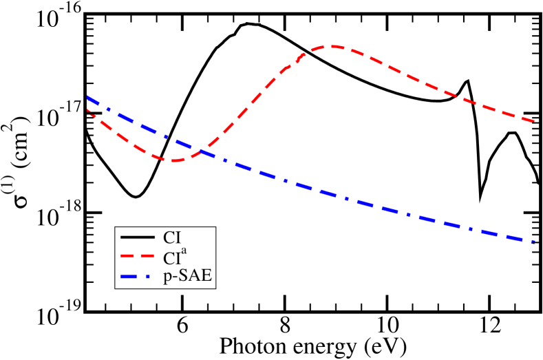
Figure 4: The one-photon ionization cross-section (within LOPT) of the H₂ B ${}^{1}\Sigma_{u}^{+}$ state for the CI (solid, black), the CI^a (red, dashed), and the p-SAE (blue, chain) basis sets.

In order to analyze the origin of the massive deviation between the SAE and the CI ionization yields it may be noted that the p-SAE approach differs from the full CI calculation only by a restriction of the configurations that are included in the CI calculation, as was outlined in Sec. II. Furthermore, the previous results have demonstrated that LOPT is applicable and the deviations between the CI and the p-SAE LOPT cross sections is practically identical to the ones found between CI-TDSE and p-SAE-TDSE. However, LOPT allows a much easier analysis of the failure of the SAE approximation, as is outlined below.

The origin of the failure of the SAE approaches can be understood from Fig. 4 that shows the one-photon ionization cross-sections within LOPT obtained from CI calculations with 3 different basis sets. The CI basis that gave converged results is again denoted as CI. As already explained, keeping in the CI basis only those configurations in which one electron remains in the 1 $\sigma_{g}$ ground-state orbital of H${}_{2}^{+}$ leads to the p-SAE model. The CI^a basis set is almost identical to the p-SAE basis set. The only difference is that it includes one additional $|1\sigma_{u}\rangle|1\sigma_{u}\rangle$ configuration in the CI calculation for the states with ${}^{1}\Sigma_{g}^{+}$ symmetry. Thus the initial B ${}^{1}\Sigma_{u}^{+}$ state is identical for the CI^a and the p-SAE basis sets. Only the final continuum states differ by the additional admixture of the single configuration ($|1\sigma_{u}\rangle|1\sigma_{u}\rangle$).

As is seen from Fig. 4, the addition of this configuration to the CI calculation of the final states leads to a substantial modification of the ionization cross-section. While for photon energies below about 6.5 eV the cross-section obtained with the CI^a is reduced compared to the p-SAE result, there is a pronounced enhancement by more than an order of magnitude at higher photon energies. While there is some evident deviation between the full CI calculation and the CI^a results, it is clear that the main failure of the SAE approximation is due to the lack of the $|1\sigma_{u}\rangle|1\sigma_{u}\rangle$ configuration in the description of the final continuum states. A further inclusion of configurations is required for achieving quantitative convergence, but the cross section does not change qualitatively. The reduction at small energies becomes more pronounced and both minima and maxima are shifted to lower photon energies. Clearly, also the adequate description of the spectral features above 11 eV due to autoionizing states requires the inclusion of additional configurations.

Based on this finding a simple semi-quantitative model for the failure of the SAE approximation can be developed. The one-photon ionization cross-section is proportional to $|\langle\psi_{f}|\hat{\rm D}|\psi_{i}\rangle|^{2}$, where $\psi_{f}$ and $\psi_{i}$ are the final and the initial state wavefunctions, respectively. $\hat{\rm D}$ is in this case the time-independent electronic dipole moment operator. In the simplest SAE approximation in which one electron is frozen during the whole process the initial state B ${}^{1}\Sigma_{u}^{+}$ can be described as a product of the (mean-field) wavefunctions $|1\sigma_{g}\rangle$ and $|1\sigma_{u}\rangle$ of H₂. A more sophisticated SAE model accounts for the proper (anti-)symmetry of the electronic wavefunction (as in the p-SAE model), but this does not change any of the following conclusions as can easily be verified. In order to keep the notation simple, the simple frozen-core model is thus pursued. The final state $\psi_{f}$ can then be approximated as $|1\sigma_{g}\rangle$ $|\epsilon\sigma_{g}\rangle$ in this simple SAE approximation and as $C_{1}(|1\sigma_{g}\rangle$ $|\epsilon\sigma_{g}\rangle)\,+\,C_{2}(|1\sigma_{u}\rangle|1\sigma_{u}\rangle)$ in a simplified two-electron model with (some) correlation. Here, $\epsilon\sigma_{g}$ describes the corresponding continuum orbital with energy $\epsilon$ and one has $|C_{1}|^{2}\,+\,|C_{2}|^{2}\,=\,1$. The dipole transition matrix element in the SAE case is

$$\langle\psi_{f}|\hat{\rm D}|\psi_{i}\rangle=\langle 1\sigma_{g};\epsilon\sigma_{g}|\hat{\rm D}|1\sigma_{g};1\sigma_{u}\rangle=\langle\epsilon\sigma_{g}|\hat{\rm D}|1\sigma_{u}\rangle\,$$ (9)

while the two-electron model yields

$$\langle\psi_{f}|\hat{\rm D}|\psi_{i}\rangle=C_{1}\langle\epsilon\sigma_{g}|\hat{\rm D}|1\sigma_{u}\rangle+C_{2}\langle 1\sigma_{u}|\hat{\rm D}|1\sigma_{g}\rangle\,.$$ (10)

Evidently, the latter gets an additional contribution from the doubly excited $|1\sigma_{u}\rangle|1\sigma_{u}\rangle$ configuration.

Of course, the size of the difference between Eqs. (9) and (10) depends on the magnitude of $C_{2}$ and the relative difference between $\langle\epsilon\sigma_{g}|\hat{\rm D}|1\sigma_{u}\rangle$ and $\langle 1\sigma_{u}|\hat{\rm D}|1\sigma_{g}\rangle$. Although correlation in the final state and thus $C_{2}$ is expected to be small, it can be compensated by the size of the dipole matrix element. Using the additional simplification of adopting H${}_{2}^{+}$ orbitals instead of the ones of H₂ one finds (with the CI^a basis) the maximum value of the coefficient $C_{2}$ to be about 0.15, and thus the maximum contribution of the $|1\sigma_{u}\rangle|1\sigma_{u}\rangle$ configuration to the continuum wavefunction to amount to about 2.25%. While this coefficient is very small, the dipole moment $\langle 1\sigma_{u}|\hat{\rm D}|1\sigma_{g}\rangle$ between two bound orbitals of similar spatial extension is on the other hand much larger than the one between the continuum orbital $\epsilon\sigma_{g}$ and the bound state $1\sigma_{u}$. While the former is found to be equal to 1.1602 a. u. at $R=2.3\,a_{0}$ (in good agreement with the results in dia:bate51 ; sfm:lin00c ), the discretized (and thus equally normalized) transition dipole matrix element $\langle n\sigma_{g}|\hat{\rm D}|1\sigma_{u}\rangle$ is found to be 0.0408 a. u. at a final-state energy corresponding to a photon energy of about 8 eV. This explains easily the dominance of the second amplitude in Eq. (10) and the failure of an SAE model.

Even a very small admixture of states like $|1\sigma_{u}\rangle|1\sigma_{u}\rangle$ due to correlation can substantially modify the one-photon cross section, since the bound-bound transition matrix elements are much larger than the bound-continuum ones. From Fig. 4 one may further conclude that the coefficient $C_{2}$ changes sign (relative to $C_{1}$) at a final-state energy at about 2 to 3 eV above the ionization threshold, since the cross section is first reduced and than enhanced compared to the one obtained with the SAE model. Clearly, a comparable effect does not occur for the electronic ground state, since all matrix elements of the type $\langle n\sigma_{g};m\sigma_{u}|\hat{\rm D}|1\sigma_{g};1\sigma_{g}\rangle$ vanish systematically for $n\neq 1$ due to the orthogonality of the orbitals; the matrix element of a one-electron operator between two Slater determinants differing by more than one orbital is zero.

IV Conclusions

On the basis of results obtained from the solution of full dimensional time-dependent Schrödinger equation describing the two electrons of H₂ exposed to an intense laser field the ionization of the first electronically excited B ${}^{1}\Sigma_{u}^{+}$ state is investigated in the one-photon regime. A large deviation is found compared to a corresponding recent calculation sfm:bart08 performed within a Koopmans’ picture based SAE approximation. It is demonstrated that also two other SAE approximations (called p-SAE and DFT-SAE) fail similarly, although DFT-SAE seemed on the first glance to yield reasonable results. However, this turned out to be accidentally caused by two partially compensating errors. On the other hand, lowest-order perturbation theory was shown to be quite adequate to reproduce the full TDSE calculations. This allowed to demonstrate that the failure of the SAE approximations is solely due to an improper description of the final continuum state, while the initial B ${}^{1}\Sigma_{u}^{+}$ state is properly described. The inclusion of a single doubly-excited configuration into the configuration-interaction calculation of the final states explains semi-quantitatively the increase of the cross section by about an order of magnitude compared to an SAE model. The present work is thus an interesting example for a dramatic effect of correlation in the final continuum states that emerges for an excited initial electronic state but is absent, if the initial state is the electronic ground state of H₂. The found effect may be observable with synchrotron radiation. However, since it is rather difficult to achieve the required target density of electronically excited states, experiments with higher photon fluxes as they are available from free-electron lasers should be advantageous.

References

- (1) J. M. J. Madey, Journal of Applied Physics 42, 1906 (1971)
- (2) A. Rudenko, L. Foucar, M. Kurka, T. Ergler, K. U. Kühnel, Y. H. Jiang, A. Voitkiv, B. Najjari, A. Kheifets, S. Lüdemann, T. Havermeier, M. Smolarski, S. Schössler, K. Cole, M. Schöffler, R. Dörner, S. Düsterer, W. Li, B. Keitel, R. Treusch, M. Gensch, C. D. Schröter, R. Moshammer, and J. Ullrich, Phys. Rev. Lett. 101, 073003 (2008)
- (3) M. Richter, M. Y. Amusia, S. V. Bobashev, T. Feigl, P. N. Juranić, M. Martins, A. A. Sorokin, and K. Tiedtke, Phys. Rev. Lett. 102, 163002 (2009)
- (4) Y. H. Jiang, A. Rudenko, M. Kurka, K. U. Kühnel, T. Ergler, L. Foucar, M. Schöffler, S. Schössler, T. Havermeier, M. Smolarski, K. Cole, R. Dörner, S. Düsterer, R. Treusch, M. Gensch, C. D. Schröter, R. Moshammer, and J. Ullrich, Phys. Rev. Lett. 102, 123002 (2009)
- (5) G. Zhu, M. Schuricke, J. Steinmann, J. Albrecht, J. Ullrich, I. Ben-Itzhak, T. J. M. Zouros, J. Colgan, M. S. Pindzola, and A. Dorn, Phys. Rev. Lett. 103, 103008 (2009)
- (6) L. V. Keldysh, Sov. Phys. JETP 20, 1307 (1965)
- (7) A. Apalategui, A. Saenz, and P. Lambropoulos, Phys. Rev. Lett. 86, 5454 (2001)
- (8) A. Apalategui and A. Saenz, J. Phys. B 35, 1909 (2002)
- (9) I. Kawata, H. Kono, Y. Fujimura, and A. D. Bandrauk, Phys. Rev. A 62, 031401(R) (2000)
- (10) M. Awasthi, Y. V. Vanne, and A. Saenz, J. Phys. B 38, 3973 (2005)
- (11) M. Awasthi and A. Saenz, J. Phys. B 39, S 389 (2006)
- (12) A. Palacios, H. Bachau, and F. Martín, Phys. Rev. Lett. 96, 143001 (2006)
- (13) Y. V. Vanne and A. Saenz, J. Mod. Opt. 55, 2665 (2008)
- (14) Y. V. Vanne and A. Saenz, Phys. Rev. A 80, 053422 (2009)
- (15) M. P. de Boer and H. G. Muller, Phys. Rev. Lett. 68, 2747 (1992)
- (16) R. R. Jones, D. W. Schumacher, and P. H. Bucksbaum, Phys. Rev. A 47, R49 (1993)
- (17) M. P. Hertlein, P. H. Bucksbaum, and H. G. Muller, J. Phys. B 30, L197 (1997)
- (18) H. G. Muller, Laser Phys. 9, 138 (1999)
- (19) T. Nubbemeyer, K. Gorling, A. Saenz, U. Eichmann, and W. Sandner, Phys. Rev. Lett. 101, 233001 (2008)
- (20) M. Awasthi, Y. V. Vanne, A. Saenz, A. Castro, and P. Decleva, Phys. Rev. A 77, 063403 (2008)
- (21) B. Manschwetus, T. Nubbemeyer, K. Gorling, G. Steinmeyer, U. Eichmann, H. Rottke, and W. Sandner, Phys. Rev. Lett. 102, 113002 (2009)
- (22) H. B. Pedersen, S. Altevogt, B. Jordon-Thaden, O. Heber, M. L. Rappaport, D. Schwalm, J. Ullrich, D. Zajfman, R. Treusch, N. Guerassimova, M. Martins, J.-T. Hoeft, M. Wellhófer, and A. Wolf, Phys. Rev. Lett. 98, 223202 (2007)
- (23) I. Dumitriu and A. Saenz, J. Phys. B 42, 165101 (2009)
- (24) A. Saenz, J. Phys. B 35, 4829 (2002)
- (25) I. Barth, J. Manz, and G. K. Paramonov, Mol. Phys. 106, 467 (2008)
- (26) J. Andruszkow, B. Aune, V. Ayvazyan, N. Baboi, R. Bakker, V. Balakin, D. Barni, A. Bazhan, M. Bernard, A. Bosotti, J. C. Bourdon, W. Brefeld, R. Brinkmann, S. Buhler, J.-P. Carneiro, M. Castellano, P. Castro, L. Catani, S. Chel, Y. Cho, S. Choroba, E. R. Colby, W. Decking, P. Den Hartog, M. Desmons, M. Dohlus, and D. Edwards, Phys. Rev. Lett. 85, 3825 (2000)
- (27) L. H. Yu, L. DiMauro, A. Doyuran, W. S. Graves, E. D. Johnson, R. Heese, S. Krinsky, H. Loos, J. B. Murphy, G. Rakowsky, J. Rose, T. Shaftan, B. Sheehy, J. Skaritka, X. J. Wang, and Z. Wu, Phys. Rev. Lett. 91, 074801 (2003)
- (28) P. Lambropoulos, P. Maragakis, and J. Zhang, Phys. Rep. 305, 203 (1998)
- (29) W. Kolos and L. Wolniewicz, J. Chem. Phys. 43, 2429 (1965)
- (30) L. Wolniewicz and K. Dressler, J. Chem. Phys. 88, 3861 (1988)
- (31) Y. V. Vanne and A. Saenz, J. Phys. B 37, 4101 (2004)
- (32) Y. V. Vanne, A. Saenz, A. Dalgarno, R. C. Forrey, P. Froelich, and S. Jonsell, Phys. Rev. A 73, 062706 (2006)
- (33) P. Lambropoulos, M. A. Kornberg, L. A. A. Nikolopoulos, and A. Saenz, in Multiphoton Processes, edited by L. F. DiMauro, R. R. Freeman, and K. C. Kulander (Melville, New York, 2000) p. 231
- (34) T. E. Sharp, Atomic Data 2, 119 (1971)
- (35) A. Saenz, Phys. Rev. A 61, 051402(R) (2000)
- (36) A. Saenz, J. Phys. B 33, 3519 (2000)
- (37) K. Harumiya, I. Kawata, H. Kono, and Y. Fujimura, J. Chem. Phys. 113, 8953 (2000)
- (38) A. Saenz, Phys. Rev. A 66, 063407 (2002)
- (39) I. Sánchez and F. Martín, J. Chem. Phys. 106, 7720 (1997)
- (40) I. Sánchez and F. Martín, J. Phys. B 30, 679 (1997)
- (41) D. R. Bates, J. Chem. Phys. 19, 1122 (1951)
- (42) J. T. Lin and T. F. Jiang, Phys. Rev. A 63, 013408 (2000)