IFT-UAM/CSIC-09-47
Edinburgh 2009/24
MKPH-T-09-18
DESY 09-153
SFB/CPP-10-01
LPT-Orsay/10-01

HQET at order 1/m1𝑚1/m: I. Non-perturbative parameters in the quenched approximation

Benoît Blossiera, Michele Della Morteb, Nicolas Garronc,d, Rainer Sommere
a Laboratoire de Physique Théorique, Bâtiment 210, Université Paris XI, F-91405 Orsay Cedex, France b Institut für Kernphysik, University of Mainz, D-55099 Mainz, Germany c Dpto Física Teórica and Instituto de Física Teórica UAM/CSIC

Universidad Autónoma de Madrid, Cantoblanco E-28049 Madrid, Spain d SUPA, School of Physics and Astronomy, Univ. of Edinburgh, EH9 3JZ, UK. e NIC, DESY, Platanenallee 6, 15738 Zeuthen, Germany
Abstract

We determine non-perturbatively the parameters of the lattice HQET Lagrangian and those of the time component of the heavy-light axial-vector current in the quenched approximation. The HQET expansion includes terms of order 1/mb1subscript𝑚b1/m_{\mathrm{b}}. Our results allow to compute, for example, the heavy-light spectrum and B-meson decay constants in the static approximation and to order 1/mb1subscript𝑚b1/m_{\mathrm{b}} in HQET. The determination of the parameters is separated into universal and non-universal parts. The universal results can be used to determine the parameters for various discretizations. The computation reported in this paper uses the plaquette gauge action and the “HYP1/2” action for the b-quark described by HQET. The parameters of the current also depend on the light-quark action, for which we choose non-perturbatively O(a)𝑂𝑎O(a)-improved Wilson fermions.

Key words: Lattice QCD; Heavy Quark Effective Theory

PACS: 12.38.Gc; 12.39.Hg; 14.40.Nd

1 Introduction

Heavy quark effective theory (HQET) was developed already quite a while ago [?,?,?,?,?]. Still it is of considerable interest today, primarily for two reasons. First it describes the asymptotic expansion of QCD observables in the limit of a large quark mass, in particular the mass of the b-quark, mbsubscript𝑚bm_{{\rm b}}. For this to be true, the observables have to be in the proper kinematical region. But in such a region, we expect the expansion in 1/mb1subscript𝑚b1/m_{\mathrm{b}} to be valid also non-perturbatively if the parameters in the effective theory are determined non-perturbatively. Understanding QCD then includes understanding the HQET limit. Steps towards establishing the expected equivalence on the non-perturbative level111Note that to our knowledge a proof of the renormalizability of HQET to all orders of perturbation theory has not yet been given. have already been carried out [?,?], but we intend to go much further, in particular through a complete treatment of 1/mb1subscript𝑚b1/m_{\mathrm{b}} corrections.

Second, flavour physics has become a precision field. No flavour physics observable has shown evidence for physics beyond the Standard Model with the presently available precision. In many cases the limiting part is the theoretical uncertainty, not the experimental one [?]. Reliable lattice computations are needed to make progress, but heavy quarks are difficult due to O((amb)n)Osuperscript𝑎subscript𝑚b𝑛{\rm O}((am_{{\rm b}})^{n}) discretization errors, where a𝑎a is the lattice spacing. In particular, if amb𝑎subscript𝑚bam_{{\rm b}} is too large the expansion in a𝑎a will break down altogether [?,?] 222The second one of these references shows the difficulty even for a charm quark. For more general discussions and more references we refer the reader to reviews [?,?,?,?,?].. Instead, in HQET the cutoff effects are O((aΛQCD)n)Osuperscript𝑎subscriptΛQCD𝑛{\rm O}((a\Lambda_{\rm QCD})^{n}); they are thus much more manageable.

QCD(L1subscript𝐿1L_{1}) matching HQET(L1subscript𝐿1L_{1}) SSF HQET(L2subscript𝐿2L_{2})
Figure 1: The strategy.

Here we present the determination of the parameters of the effective theory in a formulation where all power divergences are subtracted non-perturbatively through a matching of QCD and HQET in a small volume [?] with Schrödinger functional boundary conditions. As illustrated in Fig. 1, we then continue to larger lattice spacings through a step scaling method. Section 3 explains the details, in particular how lattice spacing errors are removed in each step. The work of [?] is here extended by a determination of all parameters in the action as well as those for the weak current A0subscript𝐴0A_{0} including the terms of order 1/mb1subscript𝑚b1/m_{\mathrm{b}}.

Our numerical implementation is done in the quenched approximation. It represents a very useful test-laboratory, in particular for the first motivation presented above: the qualitative features of the 1/mb1subscript𝑚b1/m_{\mathrm{b}} expansion will not depend on the fact that the light quarks are quenched. Applications of the parameters computed in this paper require the determination of energies and matrix elements in a large volume and will appear in separate papers, but already here we learn interesting lessons about the asymptotic convergence of the expansion. In the following section we recall the basic formulation of HQET, with a primary focus on defining the parameters of the theory and how they enter the computation of the spectrum and matrix elements. Section 3 gives a short but precise account of the strategy for the computation of the parameters. The technical Sections 4.1-4.2 discuss the numerical details of the different intermediate steps while Section 4.3 presents our main results for the HQET parameters.

2 HQET at order 1/mb1subscript𝑚b1/m_{\mathrm{b}}

In this section we define HQET including terms of order 1/mb1subscript𝑚b1/m_{\mathrm{b}}, in particular the parameters of the theory. We then show the expansion of a few observables as examples how the parameters can be used. We choose to regularise the theory on the lattice although our approach is in principle independent of the specific regularisation. Almost all formulae are established in [?]. They are repeated here for the benefit of the reader to keep the paper self-contained, but for details, such as the exact consequence of spin symmetry, the reader is referred to [?]. Terms of order 1/mb21superscriptsubscript𝑚b21/m_{\mathrm{b}}^{2} are dropped without notice.

2.1 Lagrangian

The HQET Lagrangian,

HQET(x)subscriptHQET𝑥\displaystyle{\mathscr{L}}_{\rm{HQET}}(x) =\displaystyle= stat(x)ωkin𝒪kin(x)ωspin𝒪spin(x),subscriptstat𝑥subscript𝜔kinsubscript𝒪kin𝑥subscript𝜔spinsubscript𝒪spin𝑥\displaystyle{\mathscr{L}}_{\rm{stat}}(x)-\omega_{\mathrm{kin}}{\cal O}_{\mathrm{kin}}(x)-\omega_{\mathrm{spin}}{\cal O}_{\mathrm{spin}}(x)\,, (2.1)

consists of the lowest order (static) term,

stat(x)=ψ¯h(x)D0ψh(x),subscriptstat𝑥subscript¯𝜓h𝑥subscript𝐷0subscript𝜓h𝑥{\mathscr{L}}_{\rm{stat}}(x)=\overline{\psi}_{\rm h}(x)\,D_{0}\,\psi_{\rm h}(x)\;, (2.2)

and the first order corrections

𝒪kin(x)subscript𝒪kin𝑥\displaystyle{\cal O}_{\mathrm{kin}}(x) =\displaystyle= ψ¯h(x)𝐃2ψh(x),𝒪spin(x)=ψ¯h(x)𝝈𝐁ψh(x).subscript¯𝜓h𝑥superscript𝐃2subscript𝜓h𝑥subscript𝒪spin𝑥subscript¯𝜓h𝑥𝝈𝐁subscript𝜓h𝑥\displaystyle\overline{\psi}_{\rm h}(x){\bf D}^{2}\psi_{\rm h}(x)\,,\quad{\cal O}_{\mathrm{spin}}(x)=\overline{\psi}_{\rm h}(x){\boldsymbol{\sigma}}\!\cdot\!{\bf B}\psi_{\rm h}(x)\,. (2.3)

We use the backward covariant derivative D0subscript𝐷0D_{0} as in [?] and the 4-component heavy quark field subject to the constraints P+ψh=ψh,ψ¯hP+=ψ¯hformulae-sequencesubscript𝑃subscript𝜓hsubscript𝜓hsubscript¯𝜓hsubscript𝑃subscript¯𝜓hP_{+}\psi_{\rm h}=\psi_{\rm h}\,,\;\overline{\psi}_{\rm h}P_{+}=\overline{\psi}_{\rm h} with P+=(1+γ0)/2subscript𝑃1subscript𝛾02P_{+}={(1+\gamma_{0})/{2}} and the discretized version 𝝈𝐁=k,jσkjF^kj/(2i),𝝈𝐁subscript𝑘𝑗subscript𝜎𝑘𝑗subscript^𝐹𝑘𝑗2𝑖{\boldsymbol{\sigma}}\!\cdot\!{\bf B}=\sum_{k,j}\sigma_{kj}\widehat{F}_{kj}/(2i)\,, where σkjsubscript𝜎𝑘𝑗\sigma_{kj} and the lattice (clover) field tensor F^^𝐹\widehat{F} are defined in [?]. The kinetic term 𝐃2superscript𝐃2{\bf D}^{2} is represented by the nearest neighbour covariant 3-d Laplacian. The normalization is such that the classical values of the coefficients are ωkin=ωspin=1/(2mb)subscript𝜔kinsubscript𝜔spin12subscript𝑚b\omega_{\mathrm{kin}}=\omega_{\mathrm{spin}}=1/(2m_{{\rm b}}). A bare mass mbaresubscript𝑚barem_{\rm bare} has to be added to the energy levels (e.g. the B-meson mass) computed with this Lagrangian to obtain the QCD ones (up to 1/mb21superscriptsubscript𝑚b21/m_{\mathrm{b}}^{2}). At the classical level it is mbsubscript𝑚bm_{{\rm b}}, but in the quantized theory, it has to further compensate a power divergence.

2.2 Weak axial current

For many applications, the weak, left handed, heavy-light current is needed. We here consider just the time component of the axial-vector part, A0subscript𝐴0A_{0}. The other components can be treated analogously, but so far we restricted ourselves to A0subscript𝐴0A_{0}, which is sufficient for a computation of pseudoscalar decay constants.

At the lowest order the current is form-identical to the relativistic one. At first order it is corrected by two composite fields of dimension four. The explicit form is

A0HQET(x)subscriptsuperscript𝐴HQET0𝑥\displaystyle A^{\rm HQET}_{0}(x) =\displaystyle= ZAHQET[A0stat(x)+i=12cA(i)A0(i)(x)],superscriptsubscript𝑍AHQETdelimited-[]subscriptsuperscript𝐴stat0𝑥superscriptsubscript𝑖12superscriptsubscript𝑐A𝑖subscriptsuperscript𝐴𝑖0𝑥\displaystyle Z_{\rm A}^{\rm HQET}\,[A^{\rm stat}_{0}(x)+\sum_{i=1}^{2}c_{\rm A}^{(i)}A^{(i)}_{0}(x)]\,, (2.4)
A0(1)(x)subscriptsuperscript𝐴10𝑥\displaystyle A^{(1)}_{0}(x) =\displaystyle= ψ¯l(x)12γ5γi(sisi)ψh(x),subscript¯𝜓l𝑥12subscript𝛾5subscript𝛾𝑖subscripts𝑖subscripts𝑖subscript𝜓h𝑥\displaystyle\overline{\psi}_{\rm l}(x){1\over 2}\gamma_{5}\gamma_{i}(\nabla\kern-0.5pt\smash{\raise 4.5pt\hbox{$\rm s$}}\kern-4.5pt_{i}-\overleftarrow{\nabla}\kern-0.5pt\smash{\raise 4.5pt\hbox{$\rm s$}}\kern-4.5pt_{i})\psi_{\rm h}(x)\,, (2.5)
A0(2)(x)subscriptsuperscript𝐴20𝑥\displaystyle A^{(2)}_{0}(x) =\displaystyle= i~Aistat(x),Aistat(x)=ψ¯l(x)γiγ5ψh(x),~subscript𝑖subscriptsuperscript𝐴stat𝑖𝑥subscriptsuperscript𝐴stat𝑖𝑥subscript¯𝜓l𝑥subscript𝛾𝑖subscript𝛾5subscript𝜓h𝑥\displaystyle-\widetilde{{\partial_{i}}}\,A^{\rm stat}_{i}(x)\,,\quad A^{\rm stat}_{i}(x)=\overline{\psi}_{\rm l}(x)\gamma_{i}\gamma_{5}\psi_{\rm h}(x)\,, (2.6)

where all derivatives are taken to be the symmetric nearest neighbor ones,

i~=12(i+i),si=12(i+i),si=12(i+i).\displaystyle\widetilde{{\partial_{i}}}=\hbox{$1\over 2$}({\partial_{i}}+\partial\kern-0.5pt\smash{\raise 4.5pt\hbox{$\ast$}}\kern-5.0pt_{i})\,,\quad\overleftarrow{\nabla}\kern-0.5pt\smash{\raise 4.5pt\hbox{$\rm s$}}\kern-4.5pt_{i}=\hbox{$1\over 2$}({\overleftarrow{\nabla}_{i}}+\overleftarrow{\nabla}\kern-0.5pt\smash{\raise 4.5pt\hbox{$\ast$}}\kern-4.5pt_{i})\,,\quad\nabla\kern-0.5pt\smash{\raise 4.5pt\hbox{$\rm s$}}\kern-4.5pt_{i}=\hbox{$1\over 2$}({\nabla_{i}}+\nabla\kern-0.5pt\smash{\raise 4.5pt\hbox{$\ast$}}\kern-4.5pt_{i})\,. (2.7)

By considering ZAHQETsuperscriptsubscript𝑍AHQETZ_{\rm A}^{\rm HQET} to be a function of ml/mbsubscript𝑚lsubscript𝑚bm_{\mathrm{l}}/m_{{\rm b}} with the light quark masses mlsubscript𝑚lm_{\mathrm{l}}, the above set of operators is complete after using the symmetries and the equations of motion. Since mlmbvery-much-less-thansubscript𝑚lsubscript𝑚bm_{\mathrm{l}}\lll m_{{\rm b}} and such effects are further reduced by a factor of the coupling constant α(mb)𝛼subscript𝑚b\alpha(m_{{\rm b}}) we ignore this dependence and determine ZAHQETsuperscriptsubscript𝑍AHQETZ_{\rm A}^{\rm HQET} with the light quark mass set to zero. Note that A0(2)(x)subscriptsuperscript𝐴20𝑥A^{(2)}_{0}(x) does not contribute to correlation functions and matrix elements at vanishing space-momentum. It is not needed for the computation of decay constants and has not been written down in [?]. We will also not determine its coefficient cA(2)superscriptsubscript𝑐A2c_{\rm A}^{(2)} here.

A short note on discretization errors is useful at this point. Remaining in the static approximation (ωkin=ωspin=0subscript𝜔kinsubscript𝜔spin0\omega_{\mathrm{kin}}=\omega_{\mathrm{spin}}=0), the Lagrangian has been shown to be automatically O(a)O𝑎{\rm O}(a) improved by studying its Symanzik expansion. Therefore, all energy levels are as well [?]. The zero space-momentum matrix elements of the current A0HQETsubscriptsuperscript𝐴HQET0A^{\rm HQET}_{0} are O(a)O𝑎{\rm O}(a) improved in static approximation if one sets cA(1)=acAstatsuperscriptsubscript𝑐A1𝑎superscriptsubscript𝑐Astatc_{\rm A}^{(1)}=ac_{\rm A}^{\rm stat} [?,?]. 333 At zero space momentum, partial summation can be used to bring A0(2)subscriptsuperscript𝐴20A^{(2)}_{0} into the form used in [?]. Including the 1/mb1subscript𝑚b1/m_{\mathrm{b}} terms, linear terms in a𝑎a remain absent, except for those accompanied by a factor 1/mb1subscript𝑚b1/m_{\mathrm{b}} [?]. So leading discretization errors are O(a/mb)O𝑎subscript𝑚b{\rm O}(a/m_{{\rm b}}) and O(a2)Osuperscript𝑎2{\rm O}(a^{2}).

2.3 Observables

2.3.1 Correlation functions

Observables of interest are obtained from Euclidean correlation functions in large volume. As an illustration we consider the QCD correlator

CAA(x0)=ZA2a3𝐱A0(x)(A0(0))subscript𝐶AAsubscript𝑥0superscriptsubscript𝑍A2superscript𝑎3subscript𝐱delimited-⟨⟩subscript𝐴0𝑥superscriptsubscript𝐴00\displaystyle C_{\rm AA}(x_{0})=Z_{\rm A}^{2}a^{3}\sum_{{\it\bf x}}\Big{\langle}A_{0}(x)(A_{0}(0))^{\dagger}\Big{\rangle} (2.8)

of the heavy-light axial current in QCD, Aμ=ψ¯lγμγ5ψbsubscript𝐴𝜇subscript¯𝜓lsubscript𝛾𝜇subscript𝛾5subscript𝜓bA_{\mu}=\overline{\psi}_{\rm l}\gamma_{\mu}\gamma_{5}\psi_{\rm b} (and Aμ=ψ¯bγμγ5ψlsuperscriptsubscript𝐴𝜇subscript¯𝜓bsubscript𝛾𝜇subscript𝛾5subscript𝜓lA_{\mu}^{\dagger}=-\overline{\psi}_{\rm b}\gamma_{\mu}\gamma_{5}{\psi}_{\rm l}). It is normalized by ZAsubscript𝑍AZ_{\rm A} to satisfy the chiral Ward identities [?,?]. Ignoring renormalization for a moment, an expansion in 1/mb1subscript𝑚b1/m_{\mathrm{b}} reads

CAA(x0)subscript𝐶AAsubscript𝑥0\displaystyle C_{\rm AA}(x_{0}) =\displaystyle= CAAstat(x0)+CAA(1/m)(x0)=CAAstat(x0)[1+RAA(1/m)(x0)]superscriptsubscript𝐶AAstatsubscript𝑥0superscriptsubscript𝐶AA1𝑚subscript𝑥0superscriptsubscript𝐶AAstatsubscript𝑥0delimited-[]1superscriptsubscript𝑅AA1𝑚subscript𝑥0\displaystyle C_{\rm AA}^{\mathrm{stat}}(x_{0})+C_{\rm AA}^{(1/m)}(x_{0})=C_{\rm AA}^{\mathrm{stat}}(x_{0})\,[1+R_{\rm AA}^{(1/m)}(x_{0})] (2.9)

where the notation indicates CAA(1/m)=O(1/mb)superscriptsubscript𝐶AA1𝑚O1subscript𝑚bC_{\rm AA}^{(1/m)}={\rm O}(1/m_{\mathrm{b}}). In HQET the path integral weight is expanded in 1/mb1subscript𝑚b1/m_{\mathrm{b}} and one obtains the fully renormalized expansion

CAA(x0)subscript𝐶AAsubscript𝑥0\displaystyle C_{\rm AA}(x_{0}) =\displaystyle= embarex0(ZAHQET)2[CAAstat(x0)+ωkinCAAkin(x0)+ωspinCAAspin(x0)\displaystyle{\rm e}^{-m_{\rm bare}x_{0}}(Z_{\rm A}^{\rm HQET})^{2}\,\Big{[}C_{\rm AA}^{\mathrm{stat}}(x_{0})+\omega_{\mathrm{kin}}C_{\rm AA}^{\mathrm{kin}}(x_{0})+\omega_{\mathrm{spin}}C_{\rm AA}^{\mathrm{spin}}(x_{0}) (2.10)
+cA(1)[CδAAstat(x0)+CAδAstat(x0)]]\displaystyle\qquad\qquad\qquad\qquad\;+c_{\rm A}^{(1)}[C_{\rm\delta AA}^{\mathrm{stat}}(x_{0})+C_{\rm A\delta A}^{\mathrm{stat}}(x_{0})]\Big{]}\,
\displaystyle\equiv embarex0(ZAHQET)2CAAstat(x0)×\displaystyle{\rm e}^{-m_{\rm bare}x_{0}}(Z_{\rm A}^{\rm HQET})^{2}\,C_{\rm AA}^{\mathrm{stat}}(x_{0})\times
[1+ωkinRAAkin(x0)+ωspinRAAspin(x0)+cA(1)RδA(x0)]delimited-[]1subscript𝜔kinsuperscriptsubscript𝑅AAkinsubscript𝑥0subscript𝜔spinsuperscriptsubscript𝑅AAspinsubscript𝑥0superscriptsubscript𝑐A1subscript𝑅𝛿𝐴subscript𝑥0\displaystyle\qquad\qquad\;\Big{[}1+\omega_{\mathrm{kin}}R_{\rm AA}^{\mathrm{kin}}(x_{0})+\omega_{\mathrm{spin}}R_{\rm AA}^{\mathrm{spin}}(x_{0})+c_{\rm A}^{(1)}\,R_{\delta A}(x_{0})\Big{]}\,

in terms of bare static expectation values, for example

CAAkin(x0)=a7𝐱,zA0stat(x)(A0stat(0))𝒪kin(z)stat.superscriptsubscript𝐶AAkinsubscript𝑥0superscript𝑎7subscript𝐱𝑧subscriptdelimited-⟨⟩subscriptsuperscript𝐴stat0𝑥superscriptsubscriptsuperscript𝐴stat00subscript𝒪kin𝑧stat\displaystyle C_{\rm AA}^{\mathrm{kin}}(x_{0})=a^{7}\sum_{{\it\bf x},\,z}\Big{\langle}A^{\rm stat}_{0}(x)\,(A^{\rm stat}_{0}(0))^{\dagger}\,{\cal O}_{\mathrm{kin}}(z)\Big{\rangle}_{\mathrm{stat}}\,. (2.12)

2.3.2 Spectrum and matrix elements

The spectral representation yields the large time behaviour in QCD

CAA(x0)=𝒜2emBx0[ 1+O(eΔx0)],subscript𝐶AAsubscript𝑥0superscript𝒜2superscriptesubscript𝑚Bsubscript𝑥0delimited-[]1OsuperscripteΔsubscript𝑥0\displaystyle C_{\rm AA}(x_{0})={\cal A}^{2}\,{\rm e}^{-m_{\mathrm{B}}x_{0}}\,[\,1+{\rm O}({\rm e}^{-\Delta\,x_{0}})\,]\,, (2.13)

where ΔΔ\Delta is a gap in this channel ( 2mπabsent2subscript𝑚𝜋\approx 2m_{\pi} in large volume) and 𝒜=B(𝐩=0)|A0(0)|0𝒜quantum-operator-product𝐵𝐩0subscript𝐴000{\cal A}=\langle B({\bf p}=0)|A_{0}(0)|0\rangle in the non-relativistic normalization of states B(𝐩)|B(𝐩)=2δ(𝐩𝐩)inner-product𝐵𝐩𝐵superscript𝐩2𝛿𝐩superscript𝐩\langle B({\bf p})|B({\bf p}^{\prime})\rangle=2\delta({\bf p}-{\bf p}^{\prime}) . Of course 𝒜=fBmB/2𝒜subscript𝑓Bsubscript𝑚B2{\cal A}=f_{\mathrm{B}}\sqrt{m_{\mathrm{B}}/2} is a phenomenologically interesting quantity. Again a naive expansion reads

CAA(x0)subscript𝐶AAsubscript𝑥0\displaystyle C_{\rm AA}(x_{0}) =\displaystyle= (𝒜stat)2emBstatx0[1+2𝒜(1/m)mB(1/m)x0].superscriptsuperscript𝒜stat2superscriptesuperscriptsubscript𝑚Bstatsubscript𝑥0delimited-[]12superscript𝒜1𝑚superscriptsubscript𝑚B1𝑚subscript𝑥0\displaystyle({\cal A}^{\mathrm{stat}})^{2}\,{\rm e}^{-m_{\mathrm{B}}^{\mathrm{stat}}x_{0}}[1+2{\cal A}^{(1/m)}-m_{\mathrm{B}}^{(1/m)}x_{0}]\,. (2.14)

Using the transfer matrix of the static theory, the HQET correlators (static and beyond) are easily analysed. The result is

CAAstat(x0)=(𝒜stat)2eEstatx0[ 1+O(eΔstatx0)]superscriptsubscript𝐶AAstatsubscript𝑥0superscriptsuperscript𝒜stat2superscriptesuperscript𝐸statsubscript𝑥0delimited-[]1OsuperscriptesuperscriptΔstatsubscript𝑥0\displaystyle C_{\rm AA}^{\mathrm{stat}}(x_{0})=({\cal A}^{\mathrm{stat}})^{2}\,{\rm e}^{-E^{\rm stat}x_{0}}\,[\,1+{\rm O}({\rm e}^{-\Delta^{\mathrm{stat}}\,x_{0}})\,] (2.15)

for the static term and for example

RAAkin(x0)=2𝒜kinx0Ekin+O(x0eΔstatx0)superscriptsubscript𝑅AAkinsubscript𝑥02superscript𝒜kinsubscript𝑥0superscript𝐸kinOsubscript𝑥0superscriptesuperscriptΔstatsubscript𝑥0\displaystyle R_{\rm AA}^{\mathrm{kin}}(x_{0})=2{\cal A}^{\mathrm{kin}}-x_{0}E^{\rm kin}+{\rm O}(x_{0}\,{\rm e}^{-\Delta^{\mathrm{stat}}\,x_{0}})\, (2.16)

for the kinetic correction.444 An explicit expression for Ekinsuperscript𝐸kinE^{\rm kin} is Ekinsuperscript𝐸kin\displaystyle E^{\rm kin} =\displaystyle= 12L3B|a3𝐳𝒪kin(0,𝐳)|Bstat=12B|𝒪kin(0)|Bstat,12superscript𝐿3subscriptquantum-operator-product𝐵superscript𝑎3subscript𝐳subscript𝒪kin0𝐳𝐵stat12subscriptquantum-operator-product𝐵subscript𝒪kin0𝐵stat\displaystyle-{1\over 2L^{3}}\langle B|a^{3}\sum_{{\it\bf z}}{\cal O}_{\mathrm{kin}}(0,{\it\bf z})|B\rangle_{\mathrm{stat}}=-{1\over 2}\langle B|{\cal O}_{\mathrm{kin}}(0)|B\rangle_{\mathrm{stat}}\,, (2.17) where the state |Bket𝐵|B\rangle is an eigenstate of the static transfer matrix.

A comparison to eq. (2.13) yields

mBsubscript𝑚B\displaystyle m_{\mathrm{B}} =\displaystyle= mbare+Estat+ωkinEkin+ωspinEspin,subscript𝑚baresuperscript𝐸statsubscript𝜔kinsuperscript𝐸kinsubscript𝜔spinsuperscript𝐸spin\displaystyle m_{\rm bare}+E^{\rm stat}+\omega_{\mathrm{kin}}E^{\rm kin}+\omega_{\mathrm{spin}}E^{\rm spin}\,, (2.18)
ln(𝒜r03/2)𝒜superscriptsubscript𝑟032\displaystyle\ln({\cal A}\,r_{0}^{3/2}) =\displaystyle= ln(ZAHQET)+ln(𝒜statr03/2)+cA(1)𝒜δA+ωkin𝒜kin+ωspin𝒜spin,superscriptsubscript𝑍AHQETsuperscript𝒜statsuperscriptsubscript𝑟032superscriptsubscript𝑐A1superscript𝒜𝛿𝐴subscript𝜔kinsuperscript𝒜kinsubscript𝜔spinsuperscript𝒜spin\displaystyle\ln(Z_{\rm A}^{\rm HQET})+\ln({\cal A}^{\mathrm{stat}}\,r_{0}^{3/2})+c_{\rm A}^{(1)}{\cal A}^{\delta A}+\omega_{\mathrm{kin}}{\cal A}^{\mathrm{kin}}+\omega_{\mathrm{spin}}{\cal A}^{\mathrm{spin}}\,,

where r0subscript𝑟0r_{0} is an arbitrary length-scale of the theory. Completely analogous formulae hold for the excited state masses and matrix elements. The necessary bare quantities such as Ekinsuperscript𝐸kinE^{\rm kin} can be efficiently computed with the generalized eigenvalue method [?]. We have here chosen to write the expansion of ln(𝒜r03/2)𝒜superscriptsubscript𝑟032\ln({\cal A}\,r_{0}^{3/2}) instead of 𝒜𝒜{\cal A} itself, since in this way one explicitly avoids terms quadratic in 1/mb1subscript𝑚b1/m_{\mathrm{b}}, while e.g. in eq. (2.10) terms such as ZA(1/mb)ωkinCAAkinsuperscriptsubscript𝑍A1subscript𝑚bsubscript𝜔kinsuperscriptsubscript𝐶AAkinZ_{\mathrm{A}}^{(1/m_{\mathrm{b}})}\omega_{\mathrm{kin}}C_{\rm AA}^{\mathrm{kin}} are understood to be dropped to remain consistently in order 1/mb1subscript𝑚b1/m_{\mathrm{b}}. This rule is necessary for a correct renormalization of the theory.

2.4 Properties of non-perturbative HQET parameters

Before entering the presentation of a computation of the HQET parameters, we here mention some of their properties.

2.4.1 Scheme dependence

Since we are working in the framework of an effective field theory, which has non-trivial renormalization, the parameters have to be determined by a matching performed at finite value of the expansion parameter 1/mb1subscript𝑚b1/m_{\mathrm{b}}. The truncation of the effective theory then introduces an ambiguity of order of the left out terms.

As a result the parameters such as ωkinsubscript𝜔kin\omega_{\mathrm{kin}} and ZAHQETsuperscriptsubscript𝑍AHQETZ_{\rm A}^{\rm HQET} have a dependence on the choice of the matching condition. This is a scheme dependence, analogous to the one of the usual perturbative expansion in the renormalized QCD coupling. For an explicit example consider ln(ZAHQET)superscriptsubscript𝑍AHQET\ln(Z_{\rm A}^{\rm HQET}). Evaluated in the static approximation we will denote it by ln(ZAstat)superscriptsubscript𝑍Astat\ln(Z_{\mathrm{A}}^{\mathrm{stat}}) and including all 1/mb1subscript𝑚b1/m_{\mathrm{b}} terms it is denoted as ln(ZAHQET)=ln(ZAstat)+ln(ZA(1/mb))superscriptsubscript𝑍AHQETsuperscriptsubscript𝑍Astatsuperscriptsubscript𝑍A1subscript𝑚b\ln(Z_{\rm A}^{\rm HQET})=\ln(Z_{\mathrm{A}}^{\mathrm{stat}})+\ln(Z_{\mathrm{A}}^{(1/m_{\mathrm{b}})}). The scheme dependence of ln(ZAHQET)superscriptsubscript𝑍AHQET\ln(Z_{\rm A}^{\rm HQET}) is then of order 1/mb21superscriptsubscript𝑚b21/m_{\mathrm{b}}^{2}, while the one of ln(ZAstat)superscriptsubscript𝑍Astat\ln(Z_{\mathrm{A}}^{\mathrm{stat}}) and ln(ZA(1/mb))superscriptsubscript𝑍A1subscript𝑚b\ln(Z_{\mathrm{A}}^{(1/m_{\mathrm{b}})}) individually is of order 1/mb1subscript𝑚b1/m_{\mathrm{b}}. Note that in all this discussion we are working non-perturbatively in the QCD coupling but order by order in 1/mb1subscript𝑚b1/m_{\mathrm{b}}.

2.4.2 Difference to previous renormalizations in the static approximation

In order to avoid a misunderstanding we also point out the difference to the renormalization carried out for example in [?,?]. As long as one is working just in the static approximation, the weak currents do not mix with operators of different dimensions. It is then also consistent to renormalize them perturbatively. Both to avoid ambiguities in renormalization schemes and to be able to profit from the high order continuum perturbative results [?,?], it is advantageous to first introduce the RGI current,

(ARGI)0(x)=ZA,RGIstatA0stat(x).subscriptsuperscript𝐴RGI0𝑥superscriptsubscript𝑍ARGIstatsubscriptsuperscript𝐴stat0𝑥\displaystyle(A^{\rm RGI})_{0}(x)=Z_{\rm A,RGI}^{\rm stat}\,A^{\rm stat}_{0}(x)\,. (2.20)

The renormalization constant ZA,RGIstatsuperscriptsubscript𝑍ARGIstatZ_{\rm A,RGI}^{\rm stat} has been determined non-perturbatively in [?] for the quenched case, and in [?] for two flavours of dynamical quarks.

However, here we determine ZAstatsuperscriptsubscript𝑍AstatZ_{\rm A}^{\rm stat} by a non-perturbative matching to QCD, and it is different. In fact the correspondence is

ZAstat=ZA,RGIstatCPS(Mb/Λ),superscriptsubscript𝑍Astatsuperscriptsubscript𝑍ARGIstatsubscript𝐶PSsubscript𝑀bΛ\displaystyle Z_{\rm A}^{\rm stat}=Z_{\rm A,RGI}^{\rm stat}C_{\rm PS}(M_{{\rm b}}/\Lambda)\,, (2.21)

in terms of the matching function CPSsubscript𝐶PSC_{\rm PS} introduced in [?]. In the “old” strategy of for example [?,?], functions such as CPSsubscript𝐶PSC_{\rm PS} are determined from high-order perturbation theory, while here we evaluate the full factor ZAstatsuperscriptsubscript𝑍AstatZ_{\rm A}^{\rm stat} non-perturbatively.

3 Computation of HQET parameters

ωisubscript𝜔𝑖\omega_{i} definition classical static
value value
ω1subscript𝜔1\omega_{1} mbaresubscript𝑚barem_{\rm bare} mbsubscript𝑚bm_{{\rm b}} mbarestatsuperscriptsubscript𝑚barestatm_{\rm bare}^{\mathrm{stat}}
ω2subscript𝜔2\omega_{2} ln(ZAHQET)superscriptsubscript𝑍AHQET\ln(Z_{\rm A}^{\rm HQET}) 0 ln(ZA,RGIstatCPS)superscriptsubscript𝑍ARGIstatsubscript𝐶PS\ln(Z_{\rm A,RGI}^{\rm stat}C_{\rm PS})
ω3subscript𝜔3\omega_{3} cA(1)superscriptsubscript𝑐A1c_{\rm A}^{(1)} 1/(2mb)12subscript𝑚b-1/(2m_{{\rm b}}) acAstat𝑎superscriptsubscript𝑐Astatac_{\rm A}^{\rm stat}
ω4subscript𝜔4\omega_{4} ωkinsubscript𝜔kin\omega_{\mathrm{kin}} 1/(2mb)12subscript𝑚b1/(2m_{{\rm b}}) 00
ω5subscript𝜔5\omega_{5} ωspinsubscript𝜔spin\omega_{\mathrm{spin}} 1/(2mb)12subscript𝑚b1/(2m_{{\rm b}}) 00
Table 1: Notation for HQET parameters, their values in classical and static approximation.

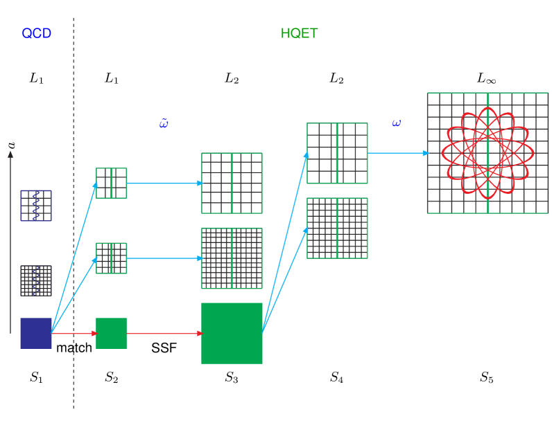
We collect all HQET parameters into one vector ω𝜔\omega with components ωi,i=1,,5formulae-sequencesubscript𝜔𝑖𝑖15\omega_{i}\,,i=1,\ldots,5 listed explicitly in Table 1. In static approximation the parameters are ω1,ω2subscript𝜔1subscript𝜔2\omega_{1},\,\omega_{2}. When 1/mb1subscript𝑚b1/m_{\mathrm{b}} corrections are included, the additional parameters in the action are ω4,ω5subscript𝜔4subscript𝜔5\omega_{4},\,\omega_{5}; moreover the previous parameters change by (partially power divergent) terms of order 1/mb1subscript𝑚b1/m_{\mathrm{b}}. The situation with ω3subscript𝜔3\omega_{3} is more intricate. It is needed for O(a)O𝑎{\rm O}(a)-improvement of the static approximation and for genuine 1/mb1subscript𝑚b1/m_{\mathrm{b}}-terms at order 1/mb1subscript𝑚b1/m_{\mathrm{b}}. We now turn to an explanation of the various steps involved in the determination of the ωisubscript𝜔𝑖\omega_{i}. Our strategy is illustrated in Fig. 2.
Refer to caption


Figure 2: Illustration of the strategy. Our numerical application uses much finer resolutions a/L𝑎𝐿a/L than those shown here. For each step i𝑖i a series of simulations Sisubscript𝑆𝑖S_{i} is necessary, they are described in the text and in Table 2.

3.1 Finite volume observables

Five observables ΦisubscriptΦ𝑖\Phi_{i} are required to determine the HQET parameters ωisubscript𝜔𝑖\omega_{i}. We choose Φi(L,M,a)subscriptΦ𝑖𝐿𝑀𝑎\Phi_{i}(L,M,a) defined from Schrödinger functional correlation functions by forming suitable renormalized combinations. They are universal, which means in particular that their continuum limit Φi(L,M,0)subscriptΦ𝑖𝐿𝑀0\Phi_{i}(L,M,0) exists.

As variables we have chosen the box size L𝐿L (which plays the rôle of a kinematical variable), the RGI mass of the heavy quark, M𝑀M, and the lattice spacing a𝑎a. Equivalent but dimensionless variables are a non-perturbative running coupling g¯(L)¯𝑔𝐿\bar{g}(L) (e.g. in the Schrödinger functional scheme), the combination z=ML𝑧𝑀𝐿z=ML and the resolution a/L𝑎𝐿a/L. The light quark masses are assumed fixed (in the numerics they are set to zero).

Most of the details of our choice follows closely [?]; for others we refer the reader to App. A. Here we note only a few properties. As L𝐿L becomes large, Φi,i=1,2formulae-sequencesubscriptΦ𝑖𝑖12\Phi_{i}\,,\;i=1,2 tend to the B-meson mass and the logarithm of the B-meson decay constant, up to kinematical constants. They are thus mainly determining ωi2subscript𝜔𝑖2\omega_{i\leq 2}. Correspondingly Φ4subscriptΦ4\Phi_{4} and Φ5subscriptΦ5\Phi_{5} allow easy access to the 1/mb1subscript𝑚b1/m_{\mathrm{b}}-parameters in the Lagrangian and Φ3subscriptΦ3\Phi_{3} to the correction term of the current with coefficient cA(1)superscriptsubscript𝑐A1c_{\rm A}^{(1)}.

By a choice of notation (e.g. considering ln(𝒜)𝒜\ln({\cal A}) instead of 𝒜𝒜{\cal A}), we arranged our finite volume observables to be linear in ω𝜔\omega,

Φ(L,M,a)=η(L,a)+ϕ(L,a)ω(M,a).Φ𝐿𝑀𝑎𝜂𝐿𝑎italic-ϕ𝐿𝑎𝜔𝑀𝑎\displaystyle\Phi(L,M,a)=\eta(L,a)+\phi(L,a)\,\omega(M,a)\,. (3.22)

By construction ϕitalic-ϕ\phi is a block diagonal matrix, which is explicitly given in terms of (bare) correlation functions in HQET. The inhomogeneous pieces ηisubscript𝜂𝑖\eta_{i} involve just correlation functions in the static approximation. Their continuum limits ηi(L,0)subscript𝜂𝑖𝐿0\eta_{i}(L,0) exist for i>2𝑖2i>2, while for i=1,2𝑖12i=1,2 additive renormalizations are necessary. They are contained in the second term of eq. (3.22). In the case i>2𝑖2i>2, the two terms of the right hand side of eq. (3.22) are then computed separately, see section 3.5.

The HQET parameters ω𝜔\omega are defined by matching at a certain value of L=L1𝐿subscript𝐿1L=L_{1} the HQET observables ΦisubscriptΦ𝑖\Phi_{i} to the corresponding values ΦiQCDsubscriptsuperscriptΦQCD𝑖\Phi^{\mathrm{QCD}}_{i} computed in QCD. These QCD observables are first extrapolated to the continuum limit (indicated by S1subscript𝑆1S_{1} in Fig. 2)

ΦiQCD(L1,M,0)=lima0ΦiQCD(L1,M,a).subscriptsuperscriptΦQCD𝑖subscript𝐿1𝑀0subscript𝑎0subscriptsuperscriptΦQCD𝑖subscript𝐿1𝑀𝑎\displaystyle\Phi^{\mathrm{QCD}}_{i}(L_{1},M,0)=\lim_{a\to 0}\Phi^{\mathrm{QCD}}_{i}(L_{1},M,a)\,. (3.23)

3.2 Matching

The matching scale L1subscript𝐿1L_{1} must be chosen such that 1/L1mbmuch-less-than1subscript𝐿1subscript𝑚b{1/L_{1}}\ll m_{{\rm b}} to allow for a precise expansion in 1/mb1subscript𝑚b1/m_{\mathrm{b}}. Moreover, we want lattice spacings of order 102fmsuperscript102fm10^{-2}\,{\rm fm} in order to keep amb<1/2𝑎subscript𝑚b12am_{{\rm b}}<1/2 while performing the continuum extrapolation eq. (3.23). These constraints lead to a box size L10.4fmsubscript𝐿10.4fmL_{1}\approx 0.4\,{\rm fm} [?,?].

The HQET parameters are then defined by imposing

Φ(L1,M,a)=ΦQCD(L1,M,0)Φsubscript𝐿1𝑀𝑎superscriptΦQCDsubscript𝐿1𝑀0\displaystyle\Phi(L_{1},M,a)=\Phi^{\mathrm{QCD}}(L_{1},M,0)\, (3.24)

for any value of the lattice spacing. By inverting eq. (3.22) one obtains

ω~(M,a)ϕ1(L1,a)[ΦQCD(L1,M,0)η(L1,a)].~𝜔𝑀𝑎superscriptitalic-ϕ1subscript𝐿1𝑎delimited-[]superscriptΦQCDsubscript𝐿1𝑀0𝜂subscript𝐿1𝑎\displaystyle\tilde{\omega}(M,a)\equiv\phi^{-1}(L_{1},a)\,[\Phi^{\mathrm{QCD}}(L_{1},M,0)-\eta(L_{1},a)]\,. (3.25)

Through our choice the matrix ϕitalic-ϕ\phi is of the form

ϕ=(CB0A),ϕ1=(C1C1BA10A1),formulae-sequenceitalic-ϕmatrix𝐶𝐵0𝐴superscriptitalic-ϕ1matrixsuperscript𝐶1superscript𝐶1𝐵superscript𝐴10superscript𝐴1\displaystyle\phi=\begin{pmatrix}C&B\\ 0&A\end{pmatrix}\,,\quad\phi^{-1}=\begin{pmatrix}C^{-1}&-C^{-1}BA^{-1}\\ 0&A^{-1}\end{pmatrix}\,, (3.26)

where C=diag(L,1)𝐶diag𝐿1C={\rm diag}(L,1). The 3×3333\times 3 sub-matrix A𝐴A has a further upper triangular structure. It is written explicitly in App. B, together with its inverse.

3.3 Step scaling

For reasonable resolutions L1/aO(10)subscript𝐿1𝑎O10L_{1}/a\geq{\rm O}(10), only lattice spacings a0.05fmless-than-or-similar-to𝑎0.05fma\lesssim 0.05\,{\rm fm} are accessible, while for standard large volume HQET computations we would also like larger a𝑎a. In order to obtain ω𝜔\omega also there, we first need Φ(L,M,0)Φ𝐿𝑀0\Phi(L,M,0) at larger L=L2𝐿subscript𝐿2L=L_{2}. We simply use the values ω~(M,a)~𝜔𝑀𝑎\tilde{\omega}(M,a) of eq. (3.25) and determine the continuum limit of the HQET observables at L2subscript𝐿2L_{2} (indicated by S3subscript𝑆3S_{3} in Fig. 2)

Φ(L2,M,0)=lima0{η(L2,a)+ϕ(L2,a)ω~(M,a)}.Φsubscript𝐿2𝑀0subscript𝑎0𝜂subscript𝐿2𝑎italic-ϕsubscript𝐿2𝑎~𝜔𝑀𝑎\displaystyle\Phi(L_{2},M,0)=\lim_{a\to 0}\left\{\eta(L_{2},a)+\phi(L_{2},a)\,\tilde{\omega}(M,a)\right\}\,. (3.27)

This can be done as long as the lattice spacing is common to the n2=L2/asubscript𝑛2subscript𝐿2𝑎n_{2}=L_{2}/a and n1=L1/asubscript𝑛1subscript𝐿1𝑎n_{1}=L_{1}/a-lattices and

s=L2/L1=n2/n1𝑠subscript𝐿2subscript𝐿1subscript𝑛2subscript𝑛1\displaystyle s=L_{2}/L_{1}=n_{2}/n_{1} (3.28)

is kept at a fixed, small, ratio.555 The ratio s𝑠s is required to be fixed for the cutoff effects to be a smooth function of a/Li𝑎subscript𝐿𝑖a/L_{i}. We choose s=2𝑠2s=2 in the numerical application. Typical resolutions are L1/a=O(10)subscript𝐿1𝑎O10L_{1}/a={\rm O}(10), see Sect. 4. This procedure which takes us from L𝐿L to sL𝑠𝐿sL with a finite scale factor s𝑠s is called step scaling [?]. The explicit forms of the step scaling functions are given in App. B.

3.4 HQET parameters

The parameters ωisubscript𝜔𝑖\omega_{i} for use in large volume (see Sect. 2.3.2) are finally obtained from

ω(M,a)ϕ1(L2,a)[Φ(L2,M,0)η(L2,a)]𝜔𝑀𝑎superscriptitalic-ϕ1subscript𝐿2𝑎delimited-[]Φsubscript𝐿2𝑀0𝜂subscript𝐿2𝑎\displaystyle\omega(M,a)\equiv\phi^{-1}(L_{2},a)\,[\Phi(L_{2},M,0)-\eta(L_{2},a)]\, (3.29)

through HQET simulations (indicated by S4subscript𝑆4S_{4} in Fig. 2) with typical resolutions L2/a=O(10)subscript𝐿2𝑎O10L_{2}/a={\rm O}(10). This results in lattice spacings of a0.1fm𝑎0.1fma\approx 0.1\,{\rm fm} and smaller, as desired for the applications. While the final results ω(M,a)𝜔𝑀𝑎\omega(M,a) do depend on all details of the regularization (gauge action etc.), the intermediate observables Φi(L2,M,0)subscriptΦ𝑖subscript𝐿2𝑀0\Phi_{i}(L_{2},M,0) may be used universally (e.g. together with an implementation of eq. (3.29) with a different regularization).

3.5 Splitting lowest order and first order in 1/mb1subscript𝑚b1/m_{\mathrm{b}}

In Sect. 2.4.1 we discussed that the splitting of a prediction into different orders of the 1/mb1subscript𝑚b1/m_{\mathrm{b}}-expansion is not unique. Nevertheless, it is of interest to organize the calculation into a static one and the remainder. In this way one can judge on the generic size of 1/mb1subscript𝑚b1/m_{\mathrm{b}} corrections and thus get some indication of the asymptotic convergence of the series. A second reason is that the static theory is O(a)O𝑎{\rm O}(a) improved when ω3subscript𝜔3\omega_{3} is included and then represents the improvement coefficient acAstat=ω3𝑎superscriptsubscript𝑐Astatsubscript𝜔3ac_{\rm A}^{\rm stat}=\omega_{3} [?]. Thus the by far dominating part of the result can be extrapolated quadratically in a𝑎a and only a small correction has to be extrapolated linearly to the continuum limit. Since a non-perturbative determination of cAstatsuperscriptsubscript𝑐Astatc_{\rm A}^{\rm stat} has not been carried out, we will here use its one-loop perturbative value [?]. We anyway carried out quadratic extrapolations in a𝑎a and then studied the effect of incomplete improvement. We will see in Sect. 4 that cAstatsuperscriptsubscript𝑐Astatc_{\rm A}^{\rm stat} is of little relevance. Therefore we profit from the O(a)O𝑎{\rm O}(a)-improvement of the static theory, irrespective of the precise value of cAstatsuperscriptsubscript𝑐Astatc_{\rm A}^{\rm stat}.

To summarize, the static approximation is defined by using exactly the same formulae as in HQET with 1/mb1subscript𝑚b1/m_{\mathrm{b}} but setting

ω3statsuperscriptsubscript𝜔3stat\displaystyle\omega_{3}^{\mathrm{stat}} =\displaystyle= acAstat𝑎superscriptsubscript𝑐Astat\displaystyle ac_{\rm A}^{\rm stat} (3.30)
ω4statsuperscriptsubscript𝜔4stat\displaystyle\omega_{4}^{\mathrm{stat}} =\displaystyle= ω5stat=0,Φi>2stat=0.formulae-sequencesuperscriptsubscript𝜔5stat0superscriptsubscriptΦ𝑖2stat0\displaystyle\omega_{5}^{\mathrm{stat}}=0\,,\quad\Phi_{i>2}^{\mathrm{stat}}=0\,. (3.31)

All quantities are determined once in this static approximation and once with 1/mb1subscript𝑚b1/m_{\mathrm{b}} terms included and then the pure 1/mb1subscript𝑚b1/m_{\mathrm{b}}-corrections are given by

Φ(1/m)=ΦΦstat,ω(1/m)=ωωstat.formulae-sequencesuperscriptΦ1𝑚ΦsuperscriptΦstatsuperscript𝜔1𝑚𝜔superscript𝜔stat\displaystyle\Phi^{(1/m)}=\Phi-\Phi^{\mathrm{stat}}\,,\;\omega^{(1/m)}=\omega-\omega^{\mathrm{stat}}\,. (3.32)

For any new observables, in particular in large volume, the static results are given by inserting ωstatsuperscript𝜔stat\omega^{\mathrm{stat}} into the expressions such as eq. (2.3.2) and the 1/mb1subscript𝑚b1/m_{\mathrm{b}}-correction by inserting ω(1/m)superscript𝜔1𝑚\omega^{(1/m)} instead. Since, as we discussed earlier everything is to be linearized in the ω𝜔\omega, the “full” result up to 1/mb21superscriptsubscript𝑚b21/m_{\mathrm{b}}^{2} is obtained from summing static and 1/mb1subscript𝑚b1/m_{\mathrm{b}}-correction or by using directly ω𝜔\omega. We finally note that even though the “full” result contains O(a)O𝑎{\rm O}(a) discretization errors, it appears justified to extrapolate numerical data with a leading correction term a2proportional-toabsentsuperscript𝑎2\propto a^{2} since the linear terms are suppressed by a small 1/mb1subscript𝑚b1/m_{\mathrm{b}} factor, which one would estimate e.g. as 1/(mbr0)1/101subscript𝑚bsubscript𝑟01101/(m_{{\rm b}}r_{0})\approx 1/10.

4 Numerical results

The numerical computations have been performed in the quenched approximation. For the QCD part we used non-perturbatively O(a𝑎a)-improved Wilson fermions [?], see [?] for details of the Schrödinger functional implementation. Two discretizations of the static quarks have been considered: the so-called HYP1 and HYP2 actions [?,?]. In order to reduce discretization effects, we have implemented tree level improvement of our QCD observables and of the HQET step scaling functions (see App. D).

Our observables depend on three periodicity angles θ0,θ1,θ2subscript𝜃0subscript𝜃1subscript𝜃2\theta_{0},\theta_{1},\theta_{2}, (see App. A). As in [?] we considered all combinations of those with θi{0, 0.5, 1.0},subscript𝜃𝑖00.51.0\theta_{i}\in\{0,\,0.5,\,1.0\}\,, θ1<θ2subscript𝜃1subscript𝜃2\theta_{1}<\theta_{2}, i.e. nine different matching conditions. For our discussion of the results and the extraction of the final HQET parameters we chose a “standard set”

θ0=0.5,θ1=0.5,θ2=1.0formulae-sequencesubscript𝜃00.5formulae-sequencesubscript𝜃10.5subscript𝜃21.0\displaystyle\theta_{0}=0.5\,,\;\theta_{1}=0.5\,,\;\theta_{2}=1.0\, (4.33)

because this yields overall the smallest statistical errors in the HQET parameters. We will comment on the spread of results with other choices for θisubscript𝜃𝑖\theta_{i} as we go along.

We summarise the different simulations needed in our strategy in Table 2.

Simulation L𝐿L Theory L/a𝐿𝑎L/a
S1subscript𝑆1S_{1} L1subscript𝐿1L_{1} QCD 40,32,24,204032242040,32,24,20
S2subscript𝑆2S_{2} L1subscript𝐿1L_{1} HQET 16,12,10,8,61612108616,12,10,8,6
S3subscript𝑆3S_{3} L2subscript𝐿2L_{2} HQET 32,24,20,16,12322420161232,24,20,16,12
S4subscript𝑆4S_{4} L2subscript𝐿2L_{2} HQET 16,12,81612816,12,8
Table 2: Summary of the simulations used in this work. Note that L1/a=16,L2/a=32formulae-sequencesubscript𝐿1𝑎16subscript𝐿2𝑎32L_{1}/a=16,\;L_{2}/a=32 are in addition to those of [?].

Since a size L=L1𝐿subscript𝐿1L=L_{1} is used for the matching (eq. (3.23), eq. (3.25)) both QCD (S1subscript𝑆1S_{1}) and HQET (S2subscript𝑆2S_{2}) are simulated in that volume. The volume of space extent L2subscript𝐿2L_{2} was simulated (in HQET), with two different sets of lattice spacings:

  • First (S3subscript𝑆3S_{3}) with the same set of lattice spacing as used in S2subscript𝑆2S_{2}, to evaluate eq. (3.27).

  • Then (S4subscript𝑆4S_{4}) with lattice spacing of order 0.050.1fm0.050.1fm0.05\ldots 0.1\,{\rm fm}, in order to compute ω(M,a)𝜔𝑀𝑎\omega(M,a) given by eq. (3.29).

The choice of the simulation parameters is described in detail in [?]; Table 3 of that paper lists those for S1subscript𝑆1S_{1}, Table A.1 of [?] the parameters of S2subscript𝑆2S_{2} and S3subscript𝑆3S_{3} and Table 6 of [?] the parameters of S4subscript𝑆4S_{4}. Here we just note that L2=2L1subscript𝐿22subscript𝐿1L_{2}=2L_{1} and L1subscript𝐿1L_{1} is fixed by the Schrödinger functional coupling g¯2(L1)=u1=3.48superscript¯𝑔2subscript𝐿1subscript𝑢13.48\bar{g}^{2}(L_{1})=u_{1}=3.48. Since this condition was implemented only within a certain precision, a small mismatch of g¯2(L)=u~1superscript¯𝑔2𝐿subscript~𝑢1\bar{g}^{2}(L)=\tilde{u}_{1} used in S1subscript𝑆1S_{1} and g¯2(L)=u1superscript¯𝑔2𝐿subscript𝑢1\bar{g}^{2}(L)=u_{1} used everywhere else has to be taken into account. This is done in complete analogy to appendix D of [?]. Without discussing the details we will quote the small corrections below.

4.1 Observables in L=L1𝐿subscript𝐿1L=L_{1}.

The considered observables naturally split into three classes according to their magnitude in the 1/mb1subscript𝑚b1/m_{\mathrm{b}} expansion, or more precisely their order in z1=(ML)1superscript𝑧1superscript𝑀𝐿1z^{-1}=(ML)^{-1}. We have Φ1=O(z),Φ24=O(1)formulae-sequencesubscriptΦ1O𝑧subscriptΦ24O1\Phi_{1}={\rm O}(z),\Phi_{2\ldots 4}={\rm O}(1) and Φ5=O(1/z)subscriptΦ5O1𝑧\Phi_{5}={\rm O}(1/z). As an illustration of the numerical determinations, in particular the continuum limit, we discuss examples of all three cases. The precise definitions of ΦisubscriptΦ𝑖\Phi_{i} are found in appendix A.

Refer to caption
Refer to caption
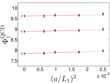
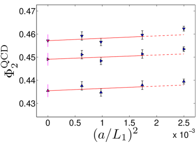
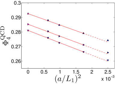
Figure 3: Continuum extrapolation of Φ1QCD(L1,M,a)subscriptsuperscriptΦQCD1subscript𝐿1𝑀𝑎\Phi^{\rm QCD}_{1}(L_{1},M,a) and Φ2QCD(L1,M,a)subscriptsuperscriptΦQCD2subscript𝐿1𝑀𝑎\Phi^{\rm QCD}_{2}(L_{1},M,a), for the three different quark masses (from the lightest to the heaviest: upward-pointing, right-pointing and downward-pointing triangle). As explained in the text, the final errors for Φ1QCD(L1,M,0)subscriptsuperscriptΦQCD1subscript𝐿1𝑀0\Phi^{\rm QCD}_{1}(L_{1},M,0) are shown on the very left. Only the data in the range of the full lines are used in the continuum extrapolations.

We recall that Φ1subscriptΦ1\Phi_{1} is simply a finite volume pseudo-scalar meson mass (up to a normalization) and determines the quark mass. In Fig. 3, we show its continuum extrapolation for our chosen values of the heavy quark mass, corresponding to z=L1M=10.4,12.1,13.3formulae-sequence𝑧subscript𝐿1𝑀10.412.113.3z=L_{1}M=10.4,12.1,13.3. We have taken into account the errors coming from the relation between the bare quark mass and the RGI quark mass. In particular, a part of this error is common to the data at all lattice spacings. It is included after the continuum extrapolation; the final error bar is shown on the left side of this plot (see also [?]). Since O(a)O𝑎{\rm O}(a) improvement is implemented, this as well as all other extrapolations of eq. (3.23) are done with the form Φi(L1,M,a)=Φi(L1,M,0)+ci(M)(a/L1)2subscriptΦ𝑖subscript𝐿1𝑀𝑎subscriptΦ𝑖subscript𝐿1𝑀0subscript𝑐𝑖𝑀superscript𝑎subscript𝐿12\Phi_{i}(L_{1},M,a)=\Phi_{i}(L_{1},M,0)+c_{i}(M)\,(a/L_{1})^{2}.

Out of the O(z0)Osuperscript𝑧0{\rm O}(z^{0}) observables, Φ2subscriptΦ2\Phi_{2} determines the normalization of the axial current. Its continuum extrapolation, eq. (3.23), is also illustrated in Fig. 3.

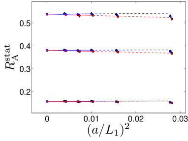
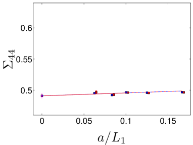
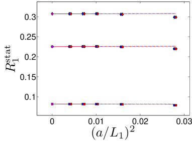
Some of the static quantities ηi(L1,a)subscript𝜂𝑖subscript𝐿1𝑎\eta_{i}(L_{1},a) have a well defined continuum limit (see appendix B). In these cases, ηi(L1,a)subscript𝜂𝑖subscript𝐿1𝑎\eta_{i}(L_{1},a) is replaced by ηi(L1,0)subscript𝜂𝑖subscript𝐿10\eta_{i}(L_{1},0) in eq. (3.25). We show examples of the determination of the continuum limit η3(L1,0)subscript𝜂3subscript𝐿10\eta_{3}(L_{1},0) and η4(L1,0)subscript𝜂4subscript𝐿10\eta_{4}(L_{1},0) in Fig. 4. The graphs use the one-loop values of the improvement coefficient[?]

cAstatsuperscriptsubscript𝑐Astat\displaystyle c_{\rm A}^{\rm stat} =\displaystyle= 0.0029g02for the HYP1 action.0.0029superscriptsubscript𝑔02for the HYP1 action\displaystyle 0.0029\,g_{0}^{2}\;\;\mbox{for the HYP1 action}\,.
cAstatsuperscriptsubscript𝑐Astat\displaystyle c_{\rm A}^{\rm stat} =\displaystyle= 0.0518g02for the HYP2 action,0.0518superscriptsubscript𝑔02for the HYP2 action\displaystyle 0.0518\,g_{0}^{2}\;\;\mbox{for the HYP2 action}\,,

As a test in how far the remaining uncertainty in cAstatsuperscriptsubscript𝑐Astatc_{\rm A}^{\rm stat} matters, we repeated the calculation setting cAstat=0superscriptsubscript𝑐Astat0c_{\rm A}^{\rm stat}=0 instead. The change is invisible in the graphs and in general, for all the continuum extrapolations of this paper, the changes in continuum values are much smaller than our quoted errors. We thus consider eq. (LABEL:e:castat1) entirely sufficient.
Refer to caption Refer to caption
Figure 4: Continuum extrapolation of η3(L1,a)=RAstat(L1,a)subscript𝜂3subscript𝐿1𝑎superscriptsubscript𝑅Astatsubscript𝐿1𝑎\eta_{3}(L_{1},a)=R_{\mathrm{A}}^{\mathrm{stat}}(L_{1},a), and η4(L1,a)=R1stat(L1,a)subscript𝜂4subscript𝐿1𝑎superscriptsubscript𝑅1statsubscript𝐿1𝑎\eta_{4}(L_{1},a)=R_{1}^{\mathrm{stat}}(L_{1},a). The three different choices (θ1,θ2)=(0,0.5),(0.5,1),(0,1.0)subscript𝜃1subscript𝜃200.50.5101.0(\theta_{1},\theta_{2})=(0,0.5),\,(0.5,1),\,(0,1.0) are represented by squares, circles, and diamonds respectively. In each case two different static actions, HYP1 (the red points, slightly shifted to the right for visibility) and HYP2 (the blue points) are used. The continuum limit is obtained by a constrained fit ηi(L1,a)=ηi(L1,0)+ci,ja2/L12subscript𝜂𝑖subscript𝐿1𝑎subscript𝜂𝑖subscript𝐿10subscript𝑐𝑖𝑗superscript𝑎2superscriptsubscript𝐿12\eta_{i}(L_{1},a)=\eta_{i}(L_{1},0)+c_{i,j}\,a^{2}/L_{1}^{2}, with j=1,2𝑗12j=1,2 for the two different actions.

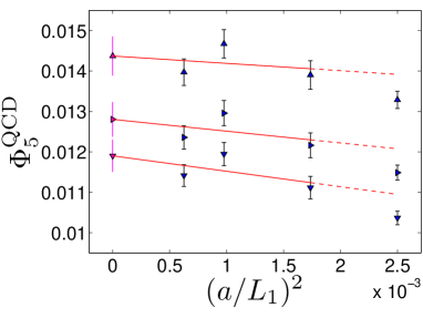
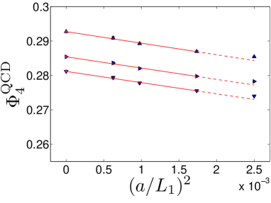
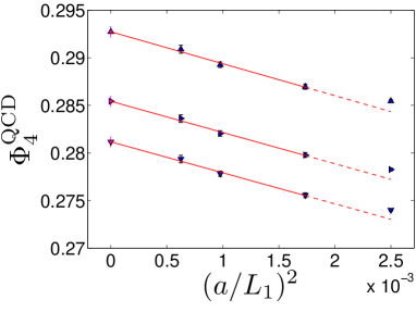
We turn now to Φ4subscriptΦ4\Phi_{4} and Φ5subscriptΦ5\Phi_{5}, needed for the determination of the 1/mb1subscript𝑚b1/m_{{\rm b}} parameters ωkinsubscript𝜔kin\omega_{\mathrm{kin}} and ωspinsubscript𝜔spin\omega_{\mathrm{spin}}. Their continuum extrapolations are shown in Fig. 5. Due to the exact spin symmetry of the static effective theory, Φ5subscriptΦ5\Phi_{5} has no static contribution. Note that both Φ5subscriptΦ5\Phi_{5} and the pure 1/mb1subscript𝑚b1/m_{\mathrm{b}} part of Φ4subscriptΦ4\Phi_{4}, obtained after subtraction of η4(L1,0)subscript𝜂4subscript𝐿10\eta_{4}(L_{1},0) (see Fig. 4), are an order of magnitude smaller than Φ4subscriptΦ4\Phi_{4}. As expected Φ4η4subscriptΦ4subscript𝜂4\Phi_{4}-\eta_{4} and Φ5subscriptΦ5\Phi_{5} are decreasing functions of the quark mass.
Refer to caption Refer to caption
Figure 5: Continuum extrapolation of the QCD observables Φ4QCD(L1,M,a)subscriptsuperscriptΦQCD4subscript𝐿1𝑀𝑎\Phi^{\mathrm{QCD}}_{4}(L_{1},M,a) and Φ5QCD(L1,M,a)subscriptsuperscriptΦQCD5subscript𝐿1𝑀𝑎\Phi^{\mathrm{QCD}}_{5}(L_{1},M,a) for the standard θ𝜃\theta’s. The three different quark masses are shown, with the same conventions as in Fig. 3.

4.2 Observables for L=L2𝐿subscript𝐿2L=L_{2}.

The step to observables in the larger volume is described by eq. (3.27). It can be broken up into several step scaling functions defined in appendix B, which individually have a continuum limit. Discussing them one by one would be too lengthy and is also not very illuminating. We follow exactly Sect. 3 and insert eq. (3.25) into eq. (3.27) lattice spacing by lattice spacing and then extrapolate a/L20𝑎subscript𝐿20a/L_{2}\to 0.

Refer to caption Refer to caption
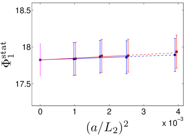
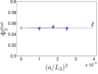
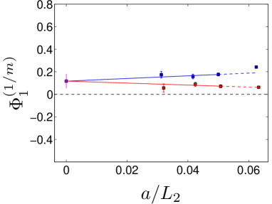
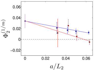
Figure 6: Continuum extrapolation of Φ1(L2)subscriptΦ1subscript𝐿2\Phi_{1}(L_{2}) and Φ2(L2)subscriptΦ2subscript𝐿2\Phi_{2}(L_{2}) for the central mass z=L1M=12.1𝑧subscript𝐿1𝑀12.1z=L_{1}M=12.1 and for the standard θ𝜃\theta’s. The scale of the y-axis of static (top) and (1/m)1𝑚{(1/m)} parts is chosen to be equal. As explained in the text, the static parts are extrapolated quadratically in a𝑎a while the (1/m)1𝑚{(1/m)} contributions are extrapolated linearly in a𝑎a. The conventions are the same as in Fig. 4.

Two examples are shown in Fig. 6. We observe that having the data for two different static actions is very useful to constrain the continuum limit, particularly so for the 1/mb1subscript𝑚b1/m_{\mathrm{b}} parts. Also the resolution L2/a=32subscript𝐿2𝑎32L_{2}/a=32 which is in addition to those of [?] helps a lot (the reader is invited to compare Φ1(1/m)superscriptsubscriptΦ11𝑚\Phi_{1}^{(1/m)} in Fig. 6 to Fig. 5 of [?]). In all cases the 1/mb1subscript𝑚b1/m_{\mathrm{b}} corrections are much smaller than the leading terms, suggesting a good asymptotic convergence of the 1/mb1subscript𝑚b1/m_{\mathrm{b}} expansion. The precision of the 1/mb1subscript𝑚b1/m_{\mathrm{b}} term is worse than the static one for Φ2subscriptΦ2\Phi_{2}, partly since the latter can be extrapolated quadratically in a𝑎a to the continuum. For Φ1subscriptΦ1\Phi_{1} this is different because the overall error contains a large piece coming from the renormalization factor determining the RGI quark mass in QCD.

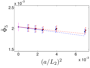
For reasons of numerical precision, Φ5subscriptΦ5\Phi_{5} (and only Φ5subscriptΦ5\Phi_{5}) is not computed exactly as described in Sect. 3. Its definition (App. A) involves the propagation of a heavy quark over a distance T=L𝑇𝐿T=L, introducing significant statistical errors for large L/a𝐿𝑎L/a in the effective theory. These become unpleasantly large in eq. (3.27), more precisely in ϕ55(L2,a)subscriptitalic-ϕ55subscript𝐿2𝑎\phi_{55}(L_{2},a). We therefore replace Φ5(L2)subscriptΦ5subscript𝐿2\Phi_{5}(L_{2}) by Φ~5(L2)subscript~Φ5subscript𝐿2\tilde{\Phi}_{5}(L_{2}) differing only by the choice T=L/2𝑇𝐿2T=L/2. An obvious question is why this is not done already for L=L1𝐿subscript𝐿1L=L_{1}. The reason is that Φ~5(L1)subscript~Φ5subscript𝐿1\tilde{\Phi}_{5}(L_{1}) turns out to be quite a bit smaller than its natural order of magnitude of O(1/z)O1𝑧{\rm O}(1/z). In such a situation O(1/z2)O1superscript𝑧2{\rm O}(1/z^{2}) terms may be numerically comparable and the 1/mb1subscript𝑚b1/m_{\mathrm{b}} expansion may be compromised in the matching step. We therefore chose the described solution, even if it is lacking elegance. 666 We have of course also determined ω~5subscript~𝜔5\tilde{\omega}_{5} from Φ~5(L1)subscript~Φ5subscript𝐿1\tilde{\Phi}_{5}(L_{1}). Despite the potentially large 1/m21superscript𝑚21/m^{2} contributions, the result for ω~5subscript~𝜔5\tilde{\omega}_{5} changes only by about 15%. The continuum extrapolation of Φ~5(L2)subscript~Φ5subscript𝐿2\tilde{\Phi}_{5}(L_{2}) is shown in Fig. 7.

Refer to caption
Figure 7: Continuum extrapolation of Φ~5(L2)subscript~Φ5subscript𝐿2\tilde{\Phi}_{5}(L_{2}) for our standard set of θisubscript𝜃𝑖\theta_{i}. The central quark mass is shown. The conventions are the same as in Fig. 4.

Since the computed Φ(L2,M,0)Φsubscript𝐿2𝑀0\Phi(L_{2},M,0) may be used in the subsequent step eq. (3.29) also with lattice discretizations which differ from ours we list Φi(L2,M,0)subscriptΦ𝑖subscript𝐿2𝑀0\Phi_{i}(L_{2},M,0) in Table 3 and Table 4. Starting from these numbers, the remaining computations to obtain the HQET parameters for a different lattice action require a very modest effort.

Φistat(L2,M,0)superscriptsubscriptΦ𝑖statsubscript𝐿2𝑀0\Phi_{i}^{\mathrm{stat}}(L_{2},M,0)
z𝑧z Φ1statsuperscriptsubscriptΦ1stat\Phi_{1}^{\mathrm{stat}} Φ2statsuperscriptsubscriptΦ2stat\Phi_{2}^{\mathrm{stat}}
10.410.410.4 15.73(20)15.732015.73(20) 0.538(4)0.53840.538(4)
12.112.112.1 17.82(22)17.822217.82(22) 0.552(4)0.55240.552(4)
13.313.313.3 19.29(24)19.292419.29(24) 0.560(4)0.56040.560(4)
Table 3: Observables Φistat(L2,M,0)superscriptsubscriptΦ𝑖statsubscript𝐿2𝑀0\Phi_{i}^{\mathrm{stat}}(L_{2},M,0) for the different values of the quark mass, and for the standard choice of θ𝜃\theta’s.
Φi(1/m)(L2,M,0)superscriptsubscriptΦ𝑖1𝑚subscript𝐿2𝑀0\Phi_{i}^{(1/m)}(L_{2},M,0)
z𝑧z Φ1(1/m)superscriptsubscriptΦ11𝑚\Phi_{1}^{(1/m)} Φ2(1/m)superscriptsubscriptΦ21𝑚\Phi_{2}^{(1/m)} Φ3(1/m)superscriptsubscriptΦ31𝑚\Phi_{3}^{(1/m)} Φ4(1/m)superscriptsubscriptΦ41𝑚\Phi_{4}^{(1/m)} Φ5(1/m)superscriptsubscriptΦ51𝑚\Phi_{5}^{(1/m)}
10.410.410.4 0.14(7)0.1470.14(7) 0.038(14)0.038140.038(14) 0.0491(23)0.0491230.0491(23) 0.0333(4)0.033340.0333(4) 0.00234(16)0.00234160.00234(16)
12.112.112.1 0.12(6)0.1260.12(6) 0.034(13)0.034130.034(13) 0.0430(22)0.0430220.0430(22) 0.0297(4)0.029740.0297(4) 0.00208(14)0.00208140.00208(14)
13.313.313.3 0.11(6)0.1160.11(6) 0.031(12)0.031120.031(12) 0.0396(21)0.0396210.0396(21) 0.0276(4)0.027640.0276(4) 0.00193(13)0.00193130.00193(13)
Table 4: Observables Φi(1/m)(L2,M,0)superscriptsubscriptΦ𝑖1𝑚subscript𝐿2𝑀0\Phi_{i}^{(1/m)}(L_{2},M,0) for the different values of the quark mass, and for the standard choice of θ𝜃\theta’s.

4.3 HQET parameters

4.3.1 Renormalization group invariant b-quark mass

For each value of z=ML1𝑧𝑀subscript𝐿1z=ML_{1}, eq. (3.29) yields the desired HQET parameters. However, for future use we want to list them for M=Mb𝑀subscript𝑀bM=M_{{\rm b}}. This saves space here and somebody doing a computation in the future does not have to fix the right quark mass. The b-quark mass was already obtained in [?] from the experimental spin-averaged Bssubscript𝐵𝑠B_{s} meson mass and r0=0.5fmsubscript𝑟00.5fmr_{0}=0.5\,{\rm fm}. Here we repeat its determination using the mass of the pseudoscalar Bssubscript𝐵sB_{\rm s} meson as experimental input. This is the natural quantity since we also start from the effective mass defined from the fAsubscript𝑓Af_{\rm A} correlator to fix the b-quark mass in the small volume. Moreover, we have improved some of the necessary steps through the finer resolution a/L2=1/32𝑎subscript𝐿2132a/L_{2}=1/32, and the use of tree level improvement (see App. D). With our new, improved determinations [?] using the GEVP method [?] we found 777 The reader might wonder why for r0Mbsubscript𝑟0subscript𝑀br_{0}M_{{\rm b}} we don’t obtain a better precision compared to the result quoted in [?]. The reason is that the uncertainty which affects the b-quark mass is dominated by the renormalization of the quark mass in QCD[?].

r0Mbstat=17.12(26),r0MbHQET=17.38(28).formulae-sequencesubscript𝑟0superscriptsubscript𝑀bstat17.1226subscript𝑟0superscriptsubscript𝑀bHQET17.3828\displaystyle r_{0}M_{{\rm b}}^{\mathrm{stat}}=17.12(26)\,,\;r_{0}M_{{\rm b}}^{\mathrm{HQET}}=17.38(28)\;. (4.35)

These results are in perfect agreement with the ones obtained when using the large volume numbers Ekin,Estatsuperscript𝐸kinsuperscript𝐸statE^{\rm kin},E^{\rm stat} of [?]. In the following we use eq. (4.35) and the knowledge of L1/r0subscript𝐿1subscript𝑟0L_{1}/r_{0} and interpolate all results quadratically in z𝑧z to zb=12.30(19)subscript𝑧b12.3019z_{\rm b}=12.30(19) in the static approximation and to zb=12.48(20)subscript𝑧b12.4820z_{\rm b}=12.48(20) at first order in 1/mb1subscript𝑚b1/m_{\mathrm{b}}.

4.3.2 Bare parameters ωisubscript𝜔𝑖\omega_{i}

Our ωisubscript𝜔𝑖\omega_{i} determined from eq. (3.29) and simulations S4subscript𝑆4S_{4} are listed in Table 5 for our standard θlimit-from𝜃\theta-combinations. The errors take all sources into account (through a jackknife analysis incorporating all steps), but one has to be aware that there are very significant correlations in the parameters. We discuss these correlations in App. C and provide them in tables available on the Internet. In static approximation a small shift proportional to u~1u1subscript~𝑢1subscript𝑢1\tilde{u}_{1}-u_{1} (see the discussion at the beginning of this section) is applied. We refer to Appendix D of [?] for the case of the b-quark mass, and with similar considerations we have evaluated the effect on the current renormalization, ln(ZAstat)superscriptsubscript𝑍Astat\ln(Z_{\rm A}^{\rm stat}). We found 888These shifts have to be added to the raw numbers computed with our simulations S1,,S4subscript𝑆1subscript𝑆4S_{1},\ldots,S_{4} but are already included in the numbers given in eq. (4.35) and in Table 5.

θ0=0,subscript𝜃00\displaystyle\theta_{0}=0\,,\,\, r0ΔMb=0.042(20),subscript𝑟0Δsubscript𝑀b0.04220\displaystyle\qquad r_{0}\Delta M_{{\rm b}}=-0.042(20)\,, Δln(ZAstat)=0.007(5),Δsuperscriptsubscript𝑍Astat0.0075\displaystyle\qquad\Delta\ln(Z_{\rm A}^{\rm stat})=0.007(5)\,, (4.36)
θ0=1/2,subscript𝜃012\displaystyle\theta_{0}=1/2\,, r0ΔMb=0.009(11),subscript𝑟0Δsubscript𝑀b0.00911\displaystyle\qquad r_{0}\Delta M_{{\rm b}}=0.009(11)\,, Δln(ZAstat)=0.008(5),Δsuperscriptsubscript𝑍Astat0.0085\displaystyle\qquad\Delta\ln(Z_{\rm A}^{\rm stat})=0.008(5)\,, (4.37)
θ0=1,subscript𝜃01\displaystyle\theta_{0}=1\,,\,\, r0ΔMb=0.150(45),subscript𝑟0Δsubscript𝑀b0.15045\displaystyle\qquad r_{0}\Delta M_{{\rm b}}=0.150(45)\,, Δln(ZAstat)=0.010(4).Δsuperscriptsubscript𝑍Astat0.0104\displaystyle\qquad\Delta\ln(Z_{\rm A}^{\rm stat})=0.010(4)\;. (4.38)
HYP1 HYP2
β𝛽\beta 6.4956 6.2885 6.0219 6.4956 6.2885 6.0219
ambarestat𝑎superscriptsubscript𝑚barestatam_{\rm bare}^{\mathrm{stat}} 0.964(12)0.964120.964(12) 1.324(17)1.324171.324(17) 2.054(25)2.054252.054(25) 0.990(12)0.990120.990(12) 1.352(17)1.352171.352(17) 2.083(25)2.083252.083(25)
ln(ZAstat)superscriptsubscript𝑍Astat\ln(Z_{\rm A}^{\rm stat}) 0.182(5)0.1825-0.182(5) 0.171(5)0.1715-0.171(5) 0.141(4)0.1414-0.141(4) 0.118(5)0.1185-0.118(5) 0.101(5)0.1015-0.101(5) 0.061(4)0.0614-0.061(4)
ambare(1/m)𝑎superscriptsubscript𝑚bare1𝑚am_{\rm bare}^{(1/m)} 0.315(6)0.3156-0.315(6) 0.264(6)0.2646-0.264(6) 0.214(8)0.2148-0.214(8) 0.328(6)0.3286-0.328(6) 0.273(6)0.2736-0.273(6) 0.215(8)0.2158-0.215(8)
ln(ZA(1/m))superscriptsubscript𝑍A1𝑚\ln(Z_{\rm A}^{(1/m)}) 0.180(28)0.180280.180(28) 0.156(24)0.156240.156(24) 0.121(20)0.121200.121(20) 0.068(27)0.068270.068(27) 0.058(24)0.058240.058(24) 0.039(20)0.039200.039(20)
cA(1)/asuperscriptsubscript𝑐A1𝑎c_{\rm A}^{(1)}/a 0.17(7)0.177-0.17(7) 0.06(5)0.065-0.06(5) 0.03(4)0.0340.03(4) 0.61(7)0.617-0.61(7) 0.46(5)0.465-0.46(5) 0.28(4)0.284-0.28(4)
ωkin/asubscript𝜔kin𝑎\omega_{\mathrm{kin}}/a 0.550(9)0.55090.550(9) 0.437(7)0.43770.437(7) 0.328(5)0.32850.328(5) 0.553(9)0.55390.553(9) 0.439(7)0.43970.439(7) 0.330(5)0.33050.330(5)
ωspin/asubscript𝜔spin𝑎\omega_{\mathrm{spin}}/a 0.76(5)0.7650.76(5) 0.59(4)0.5940.59(4) 0.43(3)0.4330.43(3) 0.87(6)0.8760.87(6) 0.71(5)0.7150.71(5) 0.55(4)0.5540.55(4)
Table 5: HQET parameters as a function of the bare coupling for the actions HYP1 and HYP2, for our choice of θisubscript𝜃𝑖\theta_{i} and for z=MbL=12.30𝑧subscript𝑀b𝐿12.30z=M_{{\rm b}}L=12.30 (static) or z=MbL=12.48𝑧subscript𝑀b𝐿12.48z=M_{{\rm b}}L=12.48. The three values of β𝛽\beta correspond to L2/a=16,12,8subscript𝐿2𝑎16128L_{2}/a=16,12,8 respectively.

Generically the bare parameters ωisubscript𝜔𝑖\omega_{i} are completely non-universal and depend on all details of the action. However here we are working in the quenched approximation. In this situation the HQET action can in principle be determined independently of the light quarks. Thus ω1,ω4subscript𝜔1subscript𝜔4\omega_{1},\omega_{4} and ω5subscript𝜔5\omega_{5} can be used for any light quark action also different from our specific one.

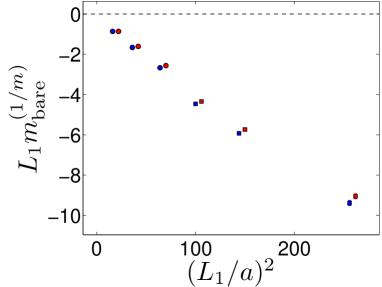
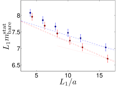
We illustrate the cutoff-dependence of ω1=mbaresubscript𝜔1subscript𝑚bare\omega_{1}=m_{\rm bare} as a function of L1/a=L1Λcutoffsubscript𝐿1𝑎subscript𝐿1subscriptΛcutoffL_{1}/a=L_{1}\Lambda_{\mathrm{cutoff}}. In Fig. 8 we show the static bare quark mass and its 1/mb1subscript𝑚b1/m_{{\rm b}} contribution in units of L1subscript𝐿1L_{1}, using L1/a=L2/(2a)subscript𝐿1𝑎subscript𝐿22𝑎L_{1}/a=L_{2}/(2a) and the data of Table 5. In addition, smaller lattice spacings are covered by including the numbers for ω~1subscript~𝜔1\tilde{\omega}_{1} from eq. (3.25). The two sets of bare parameters ω~isubscript~𝜔𝑖\tilde{\omega}_{i} and ωisubscript𝜔𝑖{\omega}_{i} differ by cutoff effects: the former are determined directly for L=L1𝐿subscript𝐿1L=L_{1} and the latter after a step scaling to L=L2𝐿subscript𝐿2L=L_{2}. Indeed these cutoff effects are visible but not dominating. The largest part of the variation with a𝑎a is due to the divergences. In the static case, the divergence is known to one-loop order from [?] (see table 1 of that paper). It is plotted for HYP1 and HYP2 using both standard (dotted lines) and boosted (dashed lines) perturbation theory, fixing the constant piece at the smallest lattice spacing. The non-perturbative results agree qualitatively with the perturbative approximations.

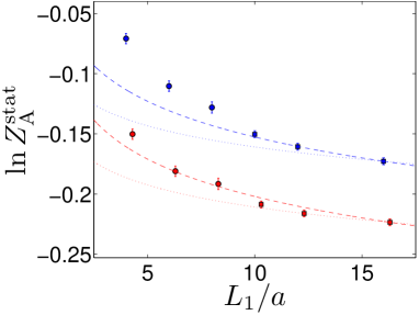
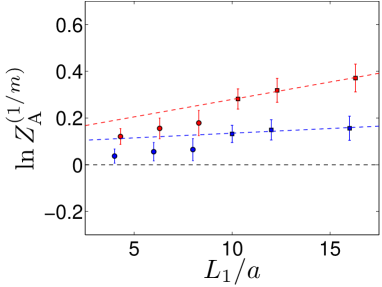
We show the equivalent plots for ln(ZAstat)superscriptsubscript𝑍Astat\ln(Z_{\rm A}^{\rm stat}) and ln(ZA(1/m))superscriptsubscript𝑍A1𝑚\ln(Z_{\rm A}^{(1/m)}) in Fig. 9. For ln(ZA(1/m))superscriptsubscript𝑍A1𝑚\ln(Z_{\rm A}^{(1/m)}) the theoretically expected 1/a1𝑎1/a divergence is not clearly visible. It either has a rather small coefficient or it is masked by terms with positive powers of the lattice spacing. For illustration we nevertheless fit a linear behaviour to ln(ZA(1/m))superscriptsubscript𝑍A1𝑚\ln(Z_{\rm A}^{(1/m)}) at the smallest three lattice spacings and extend this curve to larger ones. For ln(ZAstat)superscriptsubscript𝑍Astat\ln(Z_{\rm A}^{\rm stat}) we show the leading logarithmic divergence, ln(ZAstat)ln(a/L1)g02/(4π2)+constantsimilar-tosuperscriptsubscript𝑍Astat𝑎subscript𝐿1superscriptsubscript𝑔024superscript𝜋2constant\ln(Z_{\rm A}^{\rm stat})\sim\ln(a/L_{1})\,g_{0}^{2}/(4\pi^{2})+\rm constant, in the graph. Again the constant is adjusted to the data point at smallest a𝑎a and replacing g02superscriptsubscript𝑔02g_{0}^{2} with a boosted coupling defines the boosted perturbation theory expression.
Refer to caption Refer to caption
Figure 8: Static contribution (left) and 1/mb1subscript𝑚b1/m_{{\rm b}} correction (right) to the heavy bare quark mass. In the static case, we also show a comparison with standard and boosted perturbation theory [?], as described in the text. Data for ω1subscript𝜔1\omega_{1} from Table 5 (large volume simulations S4subscript𝑆4S_{4}) are represented by circles (the three points on the left), while ω~1subscript~𝜔1\tilde{\omega}_{1} obtained from the small volume simulations S2subscript𝑆2S_{2} are represented by squares. We use the colour blue for HYP2 and red for HYP1 (also slightly shifted to the right). The results are shown for the central mass and for the standard set of θisubscript𝜃𝑖\theta_{i}.
Refer to caption Refer to caption
Figure 9: Same as figure Fig. 8 for ln(ZA)subscript𝑍𝐴\ln(Z_{A}).

Before closing this section we would like to add a remark concerning different matching conditions. By construction, the observables ΦΦ\Phi depend on the values of the angles θisubscript𝜃𝑖\theta_{i}. Nevertheless, since the HQET parameters ωisubscript𝜔𝑖\omega_{i} are bare parameters of the HQET Lagrangian and fields, they are θ𝜃\theta independent up to truncation corrections of order (1/mb)nsuperscript1subscript𝑚b𝑛(1/m_{{\rm b}})^{n}. As one can see from eq. (3.22), this implies that the θ𝜃\theta-dependence of ΦΦ\Phi is absorbed by the ones of η𝜂\eta and ϕitalic-ϕ\phi. In practice this means that a parameter ω𝜔\omega computed in the static approximation, such as mbarestatsuperscriptsubscript𝑚barestatm_{\rm bare}^{\mathrm{stat}} or ZAstatsuperscriptsubscript𝑍AstatZ_{\rm A}^{\rm stat} exhibits a small θ𝜃\theta-dependence, but once the 1/mb1subscript𝑚b1/m_{{\rm b}} corrections are added, this dependence has to be further suppressed to order (1/mb)2superscript1subscript𝑚b2(1/m_{{\rm b}})^{2}. We checked that we obtain this behaviour in our numerical simulations. It is illustrated for the case of ω4subscript𝜔4\omega_{4} in Table 6.

L2/asubscript𝐿2𝑎L_{2}/a (θ1,θ2)=(0,0.5)subscript𝜃1subscript𝜃200.5(\theta_{1},\theta_{2})=(0,0.5) (θ1,θ2)=(0.5,1)subscript𝜃1subscript𝜃20.51(\theta_{1},\theta_{2})=(0.5,1) (θ1,θ2)=(0,1)subscript𝜃1subscript𝜃201(\theta_{1},\theta_{2})=(0,1)
Φ4(1/m)superscriptsubscriptΦ41𝑚\Phi_{4}^{{(1/m)}} 0.0098(3)0.009830.0098(3) 0.0297(4)0.029740.0297(4) 0.0395(7)0.039570.0395(7)
ωkin/asubscript𝜔kin𝑎\omega_{\mathrm{kin}}/a 161616 0.566(18)0.566180.566(18) 0.565(7)0.56570.565(7) 0.566(10)0.566100.566(10)
ωkin/asubscript𝜔kin𝑎\omega_{\mathrm{kin}}/a 121212 0.450(15)0.450150.450(15) 0.449(6)0.44960.449(6) 0.450(8)0.45080.450(8)
ωkin/asubscript𝜔kin𝑎\omega_{\mathrm{kin}}/a 888 0.339(11)0.339110.339(11) 0.338(4)0.33840.338(4) 0.338(6)0.33860.338(6)
Table 6: θ𝜃\theta– dependence of Φ4(1/m)(L2,M,0)superscriptsubscriptΦ41𝑚subscript𝐿2𝑀0\Phi_{4}^{{(1/m)}}(L_{2},M,0) and the corresponding HQET parameter ω4(M,a)=ωkin(M,a)subscript𝜔4𝑀𝑎subscript𝜔kin𝑀𝑎\omega_{4}(M,a)=\omega_{\mathrm{kin}}(M,a), for z=12.1𝑧12.1z=12.1 and the action HYP2.

5 Outlook

Our non-perturbatively computed HQET parameters show a qualitative agreement with perturbation theory as far as the leading divergence in each of the parameters is concerned (see figures 8,9), but this does not extend to the quantitative level needed for precision flavour physics.

Fortunately, in the quenched approximation, we now have the full set of parameters for HQET spectrum calculations as well as for (zero space-momentum) matrix element of A0subscript𝐴0A_{0} including the terms of order 1/mb1subscript𝑚b1/m_{\mathrm{b}} – all of them are known non-perturbatively. A detailed test of the 1/mb1subscript𝑚b1/m_{\mathrm{b}} expansion is thus possible. In companion papers we are carrying this out for the examples of the BssubscriptBs\rm B_{s} decay constant and for some mass splittings in the BssubscriptBs\rm B_{s} system; some preliminary results are described in [?]. The parameters do of course depend on our choice of discretization, but starting from Tables 3 and 4, the effort to compute them for a different regularization is very modest. Note that, as long as one remains in the quenched approximation, the parameters for the HQET action do not need to be recomputed if one uses just a light quark action differing from ours.

The small volume simulations for a determination of the parameters for Nf=2subscript𝑁𝑓2N_{f}=2 are already far advanced, see [?] for a recent account. Therefore, the situation will soon be similar with 2 flavours of dynamical fermions.

Acknowledgements. We would like to thank G. von Hippel, H. Wittig and in particular H. Simma for very useful comments on the manuscript. This work is supported by the Deutsche Forschungsgemeinschaft in the SFB/TR 09 and by the European community through EU Contract No. MRTN-CT-2006-035482, “FLAVIAnet”. N.G. acknowledges financial support from the MICINN grant FPA2006-05807, the Comunidad Autónoma de Madrid programme HEPHACOS P-ESP-00346, and participates in the Consolider-Ingenio 2010 CPAN (CSD2007-00042).

Appendix A Choice of observables

Our observables are built from Schrödinger functional [?,?] correlation functions defined exactly as in [?]. We use the renormalized boundary-to-bulk correlation function fA(x0,θ)subscript𝑓Asubscript𝑥0𝜃f_{\rm A}(x_{0},\theta) in the pseudoscalar channel as well as the boundary-to-boundary correlators f1,k1subscript𝑓1subscript𝑘1f_{1},\,k_{1}, in pseudoscalar and vector channel respectively. For their interpretation, we note in particular the rôle of θ𝜃\theta. Quark fields ψ𝜓\psi are periodic in space up to a phase eiθsuperscripte𝑖𝜃{\rm e}^{i\theta}, while ψ¯¯𝜓\overline{\psi} are periodic up to eiθsuperscripte𝑖𝜃{\rm e}^{-i\theta}. This shifts the lowest momentum of a free quark from 𝐩=0𝐩0{\bf p}=0 to 𝐩=(1,1,1)θ/L𝐩111𝜃𝐿{\bf p}=(1,1,1)\theta/L. Intermediate states to the above correlation functions have vanishing momentum, due to a projection a3𝐱superscript𝑎3subscript𝐱a^{3}\sum_{\it\bf x} and the fact that fields ψ¯1Γψ2subscript¯𝜓1Γsubscript𝜓2\overline{\psi}_{1}\Gamma\psi_{2} are periodic (with a vanishing phase). However, in the free theory, which is a relevant starting point for the interpretation in small volume, the quark carries momentum 𝐩=(1,1,1)θ/L𝐩111𝜃𝐿{\bf p}=(1,1,1)\theta/L, compensated by the opposite momentum of the anti-quark.

We form an effective energy ΓP=~0(ln(fA(x0,θ0))|(x0=T/2,T=L)\Gamma^{\rm P}=-\left.\tilde{\partial}_{0}(\ln(-f_{\rm A}(x_{0},\theta_{0}))\right|_{(x_{0}=T/2,T=L)} which approaches the heavy quark mass as it becomes very large. The logarithm of the ratio RA=ln(fA(T/2,θ1)/fA(T/2,θ2)|T=LR_{\mathrm{A}}=\left.\ln(f_{\rm A}(T/2,\theta_{1})/f_{\rm A}(T/2,\theta_{2})\right|_{T=L}  is easily seen to have a sensitivity to the coefficient ω3subscript𝜔3\omega_{3} which is approximately proportional to θ2θ1subscript𝜃2subscript𝜃1\theta_{2}-\theta_{1}: one just has to note that the covariant derivatives in eq. (2.5) acting on the quark fields are proportional to their momentum. This free theory argument is valid qualitatively in small volume. In the same way one sees that the combination R1=14(ln(f1(θ1)k1(θ1)3)ln(f1(θ2)k1(θ2)3))subscript𝑅114subscript𝑓1subscript𝜃1subscript𝑘1superscriptsubscript𝜃13subscript𝑓1subscript𝜃2subscript𝑘1superscriptsubscript𝜃23R_{1}=\hbox{$1\over 4$}\left(\ln(f_{1}(\theta_{1})k_{1}(\theta_{1})^{3})-\ln(f_{1}(\theta_{2})k_{1}(\theta_{2})^{3})\right) has a sensitivity proportional to θ22θ12superscriptsubscript𝜃22superscriptsubscript𝜃12\theta_{2}^{2}-\theta_{1}^{2} to ω4subscript𝜔4\omega_{4}, while ω5subscript𝜔5\omega_{5} does not contribute due to spin symmetry.

These qualitative considerations combined with some numerical experiments lead us to introduce

Φ=(LΓP,ln(fAf1),RA,R1,34ln(f1k1))t.Φsuperscript𝐿superscriptΓPsubscript𝑓Asubscript𝑓1subscript𝑅Asubscript𝑅134subscript𝑓1subscript𝑘1t\displaystyle\Phi=\big{(}L\Gamma^{\rm P}\,,\;\ln\left({-f_{\rm A}\over\sqrt{f_{1}}}\right)\,,\;R_{\mathrm{A}}\,,\;R_{1}\,,\;{3\over 4}\ln\left({f_{1}\over k_{1}}\right)\big{)}^{\mathrm{t}}\,. (A.39)

Appendix B Explicit form of step scaling functions

From our definitions we find immediately

Φ(L2,M,0)=Φsubscript𝐿2𝑀0absent\displaystyle\Phi(L_{2},M,0)= (B.40)
lima/L10{η(L2,a)+ϕ(L2,a)ϕ1(L1,a)[Φ(L1,M,0)η(L1,a)]},subscript𝑎subscript𝐿10𝜂subscript𝐿2𝑎italic-ϕsubscript𝐿2𝑎superscriptitalic-ϕ1subscript𝐿1𝑎delimited-[]Φsubscript𝐿1𝑀0𝜂subscript𝐿1𝑎\displaystyle\lim_{a/L_{1}\to 0}\left\{\eta(L_{2},a)+\phi(L_{2},a)\phi^{-1}(L_{1},a)[\Phi(L_{1},M,0)-\eta(L_{1},a)]\right\}\,,

where

ϕ(L2,a)ϕ1(L1,a)italic-ϕsubscript𝐿2𝑎superscriptitalic-ϕ1subscript𝐿1𝑎\displaystyle\phi(L_{2},a)\phi^{-1}(L_{1},a) =\displaystyle= (D[B(L2,a)DB(L1,a)]A1(L1,a)0A(L2,a)A1(L1,a)),matrix𝐷delimited-[]𝐵subscript𝐿2𝑎𝐷𝐵subscript𝐿1𝑎superscript𝐴1subscript𝐿1𝑎0𝐴subscript𝐿2𝑎superscript𝐴1subscript𝐿1𝑎\displaystyle\begin{pmatrix}D&[B(L_{2},a)-DB(L_{1},a)]\,A^{-1}(L_{1},a)\\ 0&A(L_{2},a)A^{-1}(L_{1},a)\end{pmatrix}\,,\; (B.41)
D𝐷\displaystyle D =\displaystyle= diag(L2/L1,1)diagsubscript𝐿2subscript𝐿11\displaystyle{\rm diag}(L_{2}/L_{1},1) (B.42)

in terms of the matrices introduced in eq. (3.26). The form

Φi(L2,M,0)subscriptΦ𝑖subscript𝐿2𝑀0\displaystyle\Phi_{i}(L_{2},M,0) =\displaystyle= DiΦi(L1,M,0)+lima/L10Σ^i(L1,a)subscript𝐷𝑖subscriptΦ𝑖subscript𝐿1𝑀0subscript𝑎subscript𝐿10subscript^Σ𝑖subscript𝐿1𝑎\displaystyle D_{i}\,\Phi_{i}(L_{1},M,0)+\lim_{a/L_{1}\to 0}\,\widehat{\Sigma}_{i}(L_{1},a)
+lima/L10j=35Σij(L1,a)[Φj(L1,M,0)ηj(L1,0)],i=1,2,formulae-sequencesubscript𝑎subscript𝐿10superscriptsubscript𝑗35subscriptΣ𝑖𝑗subscript𝐿1𝑎delimited-[]subscriptΦ𝑗subscript𝐿1𝑀0subscript𝜂𝑗subscript𝐿10𝑖12\displaystyle+\lim_{a/L_{1}\to 0}\sum_{j=3}^{5}\,\Sigma_{ij}(L_{1},a)[\Phi_{j}(L_{1},M,0)-\eta_{j}(L_{1},0)]\,,\;i=1,2\,,
Φi(L2,M,0)subscriptΦ𝑖subscript𝐿2𝑀0\displaystyle\Phi_{i}(L_{2},M,0) =\displaystyle= ηi(L2,0)+lima/L10j=35Σij(L1,M,a)[Φj(L1,M,0)ηj(L1,0)],subscript𝜂𝑖subscript𝐿20subscript𝑎subscript𝐿10superscriptsubscript𝑗35subscriptΣ𝑖𝑗subscript𝐿1𝑀𝑎delimited-[]subscriptΦ𝑗subscript𝐿1𝑀0subscript𝜂𝑗subscript𝐿10\displaystyle\eta_{i}(L_{2},0)+\lim_{a/L_{1}\to 0}\sum_{j=3}^{5}\Sigma_{ij}(L_{1},M,a)[\Phi_{j}(L_{1},M,0)-\eta_{j}(L_{1},0)]\,, (B.44)
i=35.𝑖35\displaystyle\qquad\qquad\qquad\qquad\qquad\qquad\;i=3\ldots 5\,.

then introduces step scaling functions

Σ^i(L1,a)subscript^Σ𝑖subscript𝐿1𝑎\displaystyle\widehat{\Sigma}_{i}(L_{1},a) =\displaystyle= ηi(L2,a)Diηi(L1,a),i=1,2,formulae-sequencesubscript𝜂𝑖subscript𝐿2𝑎subscript𝐷𝑖subscript𝜂𝑖subscript𝐿1𝑎𝑖12\displaystyle\eta_{i}(L_{2},a)-D_{i}\,\eta_{i}(L_{1},a)\,,\;i=1,2\,, (B.45)
Σ(L1,a)Σsubscript𝐿1𝑎\displaystyle\Sigma(L_{1},a) =\displaystyle= (D[B(L2,a)DB(L1,a)]A1(L1,a)0A(L2,a)A1(L1,a)).matrix𝐷delimited-[]𝐵subscript𝐿2𝑎𝐷𝐵subscript𝐿1𝑎superscript𝐴1subscript𝐿1𝑎0𝐴subscript𝐿2𝑎superscript𝐴1subscript𝐿1𝑎\displaystyle\begin{pmatrix}D&[B(L_{2},a)-D\,B(L_{1},a)]A^{-1}(L_{1},a)\\ 0&A(L_{2},a)\,A^{-1}(L_{1},a)\end{pmatrix}\,. (B.46)

By choosing only L1subscript𝐿1L_{1} and a𝑎a as arguments we have assumed that L2/L1=ssubscript𝐿2subscript𝐿1𝑠L_{2}/L_{1}=s is fixed (typically to s=2𝑠2s=2) which means D=diag(s,1)𝐷diag𝑠1D={\rm diag}(s,1).

The continuum limit of each element of the step scaling functions exists and the above split into two pieces is suggested by the fact that the limit a0𝑎0a\to 0 of ηi(L,M,a)subscript𝜂𝑖𝐿𝑀𝑎\eta_{i}(L,M,a) may be performed for i3𝑖3i\geq 3, while for i2𝑖2i\leq 2 there is an additive renormalization which only cancels in eq. (B.45). Splitting η𝜂\eta accordingly, η=ηa+ηb𝜂superscript𝜂𝑎superscript𝜂𝑏\eta=\eta^{a}+\eta^{b} with ηi3a=0,ηi2b=0formulae-sequencesubscriptsuperscript𝜂𝑎𝑖30subscriptsuperscript𝜂𝑏𝑖20\eta^{a}_{i\geq 3}=0\,,\;\eta^{b}_{i\leq 2}=0, we can also unify the step from L1subscript𝐿1L_{1} to L2subscript𝐿2L_{2} to (note Σ^(L,a)i3=0^Σsubscript𝐿𝑎𝑖30\widehat{\Sigma}(L,a)_{i\geq 3}=0)

Φ(L2,M,0)=ηb(L2,0)+lima/L10Σ(L1,a)[Φ(L1,M,0)ηb(L1,0)]+Σ^(L1,a).Φsubscript𝐿2𝑀0superscript𝜂𝑏subscript𝐿20subscript𝑎subscript𝐿10Σsubscript𝐿1𝑎delimited-[]Φsubscript𝐿1𝑀0superscript𝜂𝑏subscript𝐿10^Σsubscript𝐿1𝑎\displaystyle\Phi(L_{2},M,0)=\eta^{b}(L_{2},0)+\lim_{a/L_{1}\to 0}\,\Sigma(L_{1},a)[\Phi(L_{1},M,0)-\eta^{b}(L_{1},0)]+\widehat{\Sigma}(L_{1},a)\,. (B.47)

Let us now list explicit expressions for the various matrices. The expansion of the observables in HQET follows directly from the expansions detailed in section 2.3 of [?]. The inhomogeneous part is given by the static quantities

η=(LΓstat,ζA,RAstat,R1stat, 0)t,𝜂superscript𝐿superscriptΓstatsubscript𝜁Asuperscriptsubscript𝑅Astatsuperscriptsubscript𝑅1stat 0t\displaystyle\eta=\big{(}L\Gamma^{\rm stat}\,,\;\zeta_{\mathrm{A}}\,,\;R_{\mathrm{A}}^{\mathrm{stat}}\,,\;R_{1}^{\mathrm{stat}}\,,\;0\big{)}^{\mathrm{t}}\,, (B.48)

where

Γstat(L)superscriptΓstat𝐿\displaystyle\Gamma^{\rm stat}(L) =\displaystyle= 0+02(ln(fAstat(x0,θ0)))|(x0=T/2,T=L),evaluated-atsubscript0superscriptsubscript02superscriptsubscript𝑓Astatsubscript𝑥0subscript𝜃0formulae-sequencesubscript𝑥0𝑇2𝑇𝐿\displaystyle\left.-{{\partial_{0}+\partial_{0}^{*}}\over{2}}(\ln(-f_{\rm A}^{\rm stat}(x_{0},\theta_{0})))\right|_{(x_{0}=T/2,T=L)}\,, (B.49)
ζA(L)subscript𝜁A𝐿\displaystyle\zeta_{\mathrm{A}}(L) =\displaystyle= ln(fAstat(x0,θ0)f1stat(θ0))|(x0=T/2,T=L),evaluated-atsuperscriptsubscript𝑓Astatsubscript𝑥0subscript𝜃0superscriptsubscript𝑓1statsubscript𝜃0formulae-sequencesubscript𝑥0𝑇2𝑇𝐿\displaystyle\left.\ln\left({-f_{\rm A}^{\rm stat}(x_{0},\theta_{0})\over{\sqrt{f_{1}^{\rm stat}(\theta_{0})}}}\right)\right|_{(x_{0}=T/2,T=L)}\,, (B.50)
RAstat(L)superscriptsubscript𝑅Astat𝐿\displaystyle R_{\mathrm{A}}^{\mathrm{stat}}(L) =\displaystyle= ln(fAstat(x0,θ1)fAstat(x0,θ2))|(x0=T/2,T=L),evaluated-atsuperscriptsubscript𝑓Astatsubscript𝑥0subscript𝜃1superscriptsubscript𝑓Astatsubscript𝑥0subscript𝜃2formulae-sequencesubscript𝑥0𝑇2𝑇𝐿\displaystyle\left.\ln\left({f_{\rm A}^{\rm stat}(x_{0},\theta_{1})\over f_{\rm A}^{\rm stat}(x_{0},\theta_{2})}\right)\right|_{(x_{0}=T/2,T=L)}\,, (B.51)
R1stat(L)superscriptsubscript𝑅1stat𝐿\displaystyle R_{1}^{\mathrm{stat}}(L) =\displaystyle= ln(f1stat(θ1)f1stat(θ2))|T=L/2.evaluated-atsuperscriptsubscript𝑓1statsubscript𝜃1superscriptsubscript𝑓1statsubscript𝜃2𝑇𝐿2\displaystyle\left.\ln\left({f_{1}^{\rm stat}(\theta_{1})\over f_{1}^{\rm stat}(\theta_{2})}\right)\right|_{T=L/2}\,. (B.52)

Note that fAstatsuperscriptsubscript𝑓Astatf_{\rm A}^{\rm stat} does not contain the improvement term proportional to cAstatsuperscriptsubscript𝑐Astatc_{\rm A}^{\rm stat}. The improvement term is included as explained in section 3. From the definition eq. (B.45), one has

Σ^1subscript^Σ1\displaystyle\widehat{\Sigma}_{1} =\displaystyle= L2(Γstat(L2)Γstat(L1)),subscript𝐿2superscriptΓstatsubscript𝐿2superscriptΓstatsubscript𝐿1\displaystyle L_{2}(\Gamma^{\rm stat}(L_{2})-\Gamma^{\rm stat}(L_{1}))\,, (B.53)
Σ^2subscript^Σ2\displaystyle\widehat{\Sigma}_{2} =\displaystyle= ζA(L2)ζA(L1)).\displaystyle\zeta_{\mathrm{A}}(L_{2})-\zeta_{\mathrm{A}}(L_{1}))\,. (B.54)

The matrices A,B𝐴𝐵A,B which make up ϕitalic-ϕ\phi as in eq. (3.26) are

A=(RδARAkinRAspin0R1kin000ρ1spin)B=(LΓδALΓkinLΓspinρδAΨkinΨspin),formulae-sequence𝐴matrixsubscript𝑅𝛿𝐴superscriptsubscript𝑅Akinsuperscriptsubscript𝑅Aspin0superscriptsubscript𝑅1kin000superscriptsubscript𝜌1spin𝐵matrix𝐿subscriptΓ𝛿𝐴𝐿superscriptΓkin𝐿superscriptΓspinsubscript𝜌𝛿𝐴superscriptΨkinsuperscriptΨspin\displaystyle A=\begin{pmatrix}R_{\delta A}&R_{\mathrm{A}}^{\mathrm{kin}}&R_{\mathrm{A}}^{\mathrm{spin}}\\ 0&R_{1}^{\mathrm{kin}}&0\\ 0&0&\rho_{1}^{\mathrm{spin}}\end{pmatrix}\quad B=\begin{pmatrix}L\Gamma_{\delta A}&L\Gamma^{\rm kin}&L\Gamma^{\rm spin}\\ \rho_{\delta A}&\Psi^{\mathrm{kin}}&\Psi^{\mathrm{spin}}\end{pmatrix}\,, (B.55)

where

Γy(L)superscriptΓy𝐿\displaystyle\Gamma^{\rm y}(L) =\displaystyle= 0+02(fAy(x0,θ0)/fAstat(x0,θ0))|(x0=T/2,T=L),evaluated-atsubscript0superscriptsubscript02superscriptsubscript𝑓Aysubscript𝑥0subscript𝜃0superscriptsubscript𝑓Astatsubscript𝑥0subscript𝜃0formulae-sequencesubscript𝑥0𝑇2𝑇𝐿\displaystyle-\left.{{\partial_{0}+\partial_{0}^{*}}\over{2}}(f_{\rm A}^{\mathrm{y}}(x_{0},\theta_{0})/f_{\rm A}^{\rm stat}(x_{0},\theta_{0}))\right|_{(x_{0}=T/2,T=L)}\,, (B.56)
ΓδA(L)subscriptΓ𝛿𝐴𝐿\displaystyle\Gamma_{\delta A}(L) =\displaystyle= 0+02(fδAstat(x0,θ0)/fAstat(x0,θ0))|(x0=T/2,T=L),evaluated-atsubscript0superscriptsubscript02superscriptsubscript𝑓𝛿Astatsubscript𝑥0subscript𝜃0superscriptsubscript𝑓Astatsubscript𝑥0subscript𝜃0formulae-sequencesubscript𝑥0𝑇2𝑇𝐿\displaystyle-\left.{{\partial_{0}+\partial_{0}^{*}}\over{2}}(f_{\delta\rm A}^{\rm stat}(x_{0},\theta_{0})/f_{\rm A}^{\rm stat}(x_{0},\theta_{0}))\right|_{(x_{0}=T/2,T=L)}\,, (B.57)
Ψy(L)superscriptΨy𝐿\displaystyle\Psi^{\mathrm{y}}(L) =\displaystyle= (fAy(x0,θ0)fAstat(x0,θ0)12f1y(θ0)f1stat(θ0))|(x0=T/2,T=L),evaluated-atsuperscriptsubscript𝑓Aysubscript𝑥0subscript𝜃0superscriptsubscript𝑓Astatsubscript𝑥0subscript𝜃012superscriptsubscript𝑓1ysubscript𝜃0superscriptsubscript𝑓1statsubscript𝜃0formulae-sequencesubscript𝑥0𝑇2𝑇𝐿\displaystyle\left.\left({f_{\rm A}^{\mathrm{y}}(x_{0},\theta_{0})\over f_{\rm A}^{\rm stat}(x_{0},\theta_{0})}-{1\over 2}{f_{1}^{\mathrm{y}}(\theta_{0})\over f_{1}^{\rm stat}(\theta_{0})}\right)\right|_{(x_{0}=T/2,T=L)}\,, (B.58)
ρ1y(L)superscriptsubscript𝜌1y𝐿\displaystyle\rho_{1}^{\rm y}(L) =\displaystyle= f1y(θ0)f1stat(θ0)|T=L/2,evaluated-atsuperscriptsubscript𝑓1ysubscript𝜃0superscriptsubscript𝑓1statsubscript𝜃0𝑇𝐿2\displaystyle\left.{f_{1}^{\mathrm{y}}(\theta_{0})\over f_{1}^{\rm stat}(\theta_{0})}\right|_{T=L/2}\,, (B.59)
ρδA(L)subscript𝜌𝛿𝐴𝐿\displaystyle\rho_{\delta A}(L) =\displaystyle= fδAstat(x0,θ0)fAstat(x0,θ0)|(x0=T/2,T=L),evaluated-atsuperscriptsubscript𝑓𝛿Astatsubscript𝑥0subscript𝜃0superscriptsubscript𝑓Astatsubscript𝑥0subscript𝜃0formulae-sequencesubscript𝑥0𝑇2𝑇𝐿\displaystyle\left.{f_{\delta\rm A}^{\rm stat}(x_{0},\theta_{0})\over f_{\rm A}^{\rm stat}(x_{0},\theta_{0})}\right|_{(x_{0}=T/2,T=L)}\,, (B.60)
RAy(L)superscriptsubscript𝑅Ay𝐿\displaystyle R_{\mathrm{A}}^{\mathrm{y}}(L) =\displaystyle= (fAy(x0,θ1)fAstat(x0,θ1)fAy(x0,θ2)fAstat(x0,θ2))|(x0=T/2,T=L),evaluated-atsuperscriptsubscript𝑓Aysubscript𝑥0subscript𝜃1superscriptsubscript𝑓Astatsubscript𝑥0subscript𝜃1superscriptsubscript𝑓Aysubscript𝑥0subscript𝜃2superscriptsubscript𝑓Astatsubscript𝑥0subscript𝜃2formulae-sequencesubscript𝑥0𝑇2𝑇𝐿\displaystyle\left.\left({f_{\rm A}^{\mathrm{y}}(x_{0},\theta_{1})\over f_{\rm A}^{\rm stat}(x_{0},\theta_{1})}-{f_{\rm A}^{\mathrm{y}}(x_{0},\theta_{2})\over f_{\rm A}^{\rm stat}(x_{0},\theta_{2})}\right)\right|_{(x_{0}=T/2,T=L)}\,, (B.61)
RδA(L)subscript𝑅𝛿𝐴𝐿\displaystyle R_{\delta A}(L) =\displaystyle= (fδAstat(x0,θ1)fAstat(x0,θ1)fδAstat(x0,θ2)fAstat(x0,θ2))|(x0=T/2,T=L),evaluated-atsuperscriptsubscript𝑓𝛿Astatsubscript𝑥0subscript𝜃1superscriptsubscript𝑓Astatsubscript𝑥0subscript𝜃1superscriptsubscript𝑓𝛿Astatsubscript𝑥0subscript𝜃2superscriptsubscript𝑓Astatsubscript𝑥0subscript𝜃2formulae-sequencesubscript𝑥0𝑇2𝑇𝐿\displaystyle\left.\left({f_{\delta\rm A}^{\rm stat}(x_{0},\theta_{1})\over f_{\rm A}^{\rm stat}(x_{0},\theta_{1})}-{f_{\delta\rm A}^{\rm stat}(x_{0},\theta_{2})\over f_{\rm A}^{\rm stat}(x_{0},\theta_{2})}\right)\right|_{(x_{0}=T/2,T=L)}\,, (B.62)
R1y(L)superscriptsubscript𝑅1y𝐿\displaystyle R_{1}^{\mathrm{y}}(L) =\displaystyle= (f1y(θ1)f1stat(θ1)f1y(θ2)f1stat(θ2))|T=L/2.evaluated-atsuperscriptsubscript𝑓1ysubscript𝜃1superscriptsubscript𝑓1statsubscript𝜃1superscriptsubscript𝑓1ysubscript𝜃2superscriptsubscript𝑓1statsubscript𝜃2𝑇𝐿2\displaystyle\left.\left({f_{1}^{\mathrm{y}}(\theta_{1})\over f_{1}^{\rm stat}(\theta_{1})}-{f_{1}^{\mathrm{y}}(\theta_{2})\over f_{1}^{\rm stat}(\theta_{2})}\right)\right|_{T=L/2}\,. (B.63)

In order to avoid unnecessary repetitions, we have used the shortcut

y{kin,spin}.ykinspin\displaystyle\mathrm{y}\in\{\mathrm{kin},\mathrm{spin}\}\,. (B.64)

in the previous formulae. From our definitions we obtain

A1=(1/RδAK12K1301/R1kin0001/ρ1spin),superscript𝐴1matrix1subscript𝑅𝛿𝐴subscript𝐾12subscript𝐾1301superscriptsubscript𝑅1kin0001superscriptsubscript𝜌1spin\displaystyle A^{-1}=\begin{pmatrix}1/R_{\delta A}&K_{12}&K_{13}\\ 0&1/R_{1}^{\mathrm{kin}}&0\\ 0&0&1/\rho_{1}^{\mathrm{spin}}\end{pmatrix}\,,\quad (B.65)
K12=RAkinR1kinRδA,K13=RAspinρ1spinRδA,formulae-sequencesubscript𝐾12superscriptsubscript𝑅Akinsuperscriptsubscript𝑅1kinsubscript𝑅𝛿𝐴subscript𝐾13superscriptsubscript𝑅Aspinsuperscriptsubscript𝜌1spinsubscript𝑅𝛿𝐴\displaystyle K_{12}={-R_{\mathrm{A}}^{\mathrm{kin}}\over R_{1}^{\mathrm{kin}}R_{\delta A}}\,,\;K_{13}={-R_{\mathrm{A}}^{\mathrm{spin}}\over\rho_{1}^{\mathrm{spin}}R_{\delta A}}\,, (B.66)

and

[B(L2,a)DB(L1,a)]A1(L1,a)=(Σ13Σ14Σ15Σ23Σ24Σ25),delimited-[]𝐵subscript𝐿2𝑎𝐷𝐵subscript𝐿1𝑎superscript𝐴1subscript𝐿1𝑎matrixsubscriptΣ13subscriptΣ14subscriptΣ15subscriptΣ23subscriptΣ24subscriptΣ25\displaystyle[B(L_{2},a)-D\,B(L_{1},a)]A^{-1}(L_{1},a)=\begin{pmatrix}\Sigma_{13}&\Sigma_{14}&\Sigma_{15}\\ \Sigma_{23}&\Sigma_{24}&\Sigma_{25}\\ \end{pmatrix}\,, (B.67)
A(L2,a)A1(L1,a)=(Σ33Σ34Σ350Σ44000Σ55),𝐴subscript𝐿2𝑎superscript𝐴1subscript𝐿1𝑎matrixsubscriptΣ33subscriptΣ34subscriptΣ350subscriptΣ44000subscriptΣ55\displaystyle A(L_{2},a)\,A^{-1}(L_{1},a)=\begin{pmatrix}\Sigma_{33}&\Sigma_{34}&\Sigma_{35}\\ 0&\Sigma_{44}&0\\ 0&0&\Sigma_{55}\end{pmatrix}\,, (B.68)

with

Σ13subscriptΣ13\displaystyle\Sigma_{13} =\displaystyle= L2(ΓδA(L2)ΓδA(L1))/RδA(L1),subscript𝐿2subscriptΓ𝛿𝐴subscript𝐿2subscriptΓ𝛿𝐴subscript𝐿1subscript𝑅𝛿𝐴subscript𝐿1\displaystyle L_{2}(\Gamma_{\delta A}(L_{2})-\Gamma_{\delta A}(L_{1}))/R_{\delta A}(L_{1})\,,
Σ14subscriptΣ14\displaystyle\Sigma_{14} =\displaystyle= L2(ΓδA(L2)ΓδA(L1))K12(L1)+L2(Γkin(L2)Γkin(L1))/R1kin(L1),subscript𝐿2subscriptΓ𝛿𝐴subscript𝐿2subscriptΓ𝛿𝐴subscript𝐿1subscript𝐾12subscript𝐿1subscript𝐿2superscriptΓkinsubscript𝐿2superscriptΓkinsubscript𝐿1superscriptsubscript𝑅1kinsubscript𝐿1\displaystyle L_{2}(\Gamma_{\delta A}(L_{2})-\Gamma_{\delta A}(L_{1}))\,K_{12}(L_{1})+L_{2}(\Gamma^{\rm kin}(L_{2})-\Gamma^{\rm kin}(L_{1}))/R_{1}^{\mathrm{kin}}(L_{1})\,,
Σ15subscriptΣ15\displaystyle\Sigma_{15} =\displaystyle= L2(ΓδA(L2)ΓδA(L1))K13(L1)+L2(Γspin(L2)Γspin(L1))/ρ1spin(L1),subscript𝐿2subscriptΓ𝛿𝐴subscript𝐿2subscriptΓ𝛿𝐴subscript𝐿1subscript𝐾13subscript𝐿1subscript𝐿2superscriptΓspinsubscript𝐿2superscriptΓspinsubscript𝐿1superscriptsubscript𝜌1spinsubscript𝐿1\displaystyle L_{2}(\Gamma_{\delta A}(L_{2})-\Gamma_{\delta A}(L_{1}))\,K_{13}(L_{1})+L_{2}(\Gamma^{\rm spin}(L_{2})-\Gamma^{\rm spin}(L_{1}))/\rho_{1}^{\mathrm{spin}}(L_{1})\,,
Σ23subscriptΣ23\displaystyle\Sigma_{23} =\displaystyle= (ρδA(L2)ρδA(L1))/RδA(L1),subscript𝜌𝛿𝐴subscript𝐿2subscript𝜌𝛿𝐴subscript𝐿1subscript𝑅𝛿𝐴subscript𝐿1\displaystyle(\rho_{\delta A}(L_{2})-\rho_{\delta A}(L_{1}))/R_{\delta A}(L_{1})\,,
Σ24subscriptΣ24\displaystyle\Sigma_{24} =\displaystyle= (ρδA(L2)ρδA(L1))K12(L1)+(Ψkin(L2)Ψkin(L1))/R1kin(L1),subscript𝜌𝛿𝐴subscript𝐿2subscript𝜌𝛿𝐴subscript𝐿1subscript𝐾12subscript𝐿1superscriptΨkinsubscript𝐿2superscriptΨkinsubscript𝐿1superscriptsubscript𝑅1kinsubscript𝐿1\displaystyle(\rho_{\delta A}(L_{2})-\rho_{\delta A}(L_{1}))\,K_{12}(L_{1})+(\Psi^{\mathrm{kin}}(L_{2})-\Psi^{\mathrm{kin}}(L_{1}))/R_{1}^{\mathrm{kin}}(L_{1})\,,
Σ25subscriptΣ25\displaystyle\Sigma_{25} =\displaystyle= (ρδA(L2)ρδA(L1))K13(L1)+(Ψspin(L2)Ψspin(L1))/ρ1spin(L1),subscript𝜌𝛿𝐴subscript𝐿2subscript𝜌𝛿𝐴subscript𝐿1subscript𝐾13subscript𝐿1superscriptΨspinsubscript𝐿2superscriptΨspinsubscript𝐿1superscriptsubscript𝜌1spinsubscript𝐿1\displaystyle(\rho_{\delta A}(L_{2})-\rho_{\delta A}(L_{1}))\,K_{13}(L_{1})+(\Psi^{\mathrm{spin}}(L_{2})-\Psi^{\mathrm{spin}}(L_{1}))/\rho_{1}^{\mathrm{spin}}(L_{1})\,,

and

Σ33subscriptΣ33\displaystyle\Sigma_{33} =\displaystyle= RδA(L2)/RδA(L1),subscript𝑅𝛿𝐴subscript𝐿2subscript𝑅𝛿𝐴subscript𝐿1\displaystyle R_{\delta A}(L_{2})/R_{\delta A}(L_{1})\,,
Σ34subscriptΣ34\displaystyle\Sigma_{34} =\displaystyle= RδA(L2)K12(L1)+RAkin(L2)/R1kin(L1),subscript𝑅𝛿𝐴subscript𝐿2subscript𝐾12subscript𝐿1superscriptsubscript𝑅Akinsubscript𝐿2superscriptsubscript𝑅1kinsubscript𝐿1\displaystyle R_{\delta A}(L_{2})K_{12}(L_{1})+R_{\mathrm{A}}^{\mathrm{kin}}(L_{2})/R_{1}^{\mathrm{kin}}(L_{1})\,,
Σ35subscriptΣ35\displaystyle\Sigma_{35} =\displaystyle= RδA(L2)K13(L1)+RAspin(L2)/ρ1spin(L1),subscript𝑅𝛿𝐴subscript𝐿2subscript𝐾13subscript𝐿1superscriptsubscript𝑅Aspinsubscript𝐿2superscriptsubscript𝜌1spinsubscript𝐿1\displaystyle R_{\delta A}(L_{2})K_{13}(L_{1})+R_{\mathrm{A}}^{\mathrm{spin}}(L_{2})/\rho_{1}^{\mathrm{spin}}(L_{1})\,,
Σ44subscriptΣ44\displaystyle\Sigma_{44} =\displaystyle= R1kin(L2)/R1kin(L1),superscriptsubscript𝑅1kinsubscript𝐿2superscriptsubscript𝑅1kinsubscript𝐿1\displaystyle R_{1}^{\mathrm{kin}}(L_{2})/R_{1}^{\mathrm{kin}}(L_{1})\,,
Σ55subscriptΣ55\displaystyle\Sigma_{55} =\displaystyle= ρ1spin(L2)/R1spin(L1).superscriptsubscript𝜌1spinsubscript𝐿2superscriptsubscript𝑅1spinsubscript𝐿1\displaystyle\rho_{1}^{\mathrm{spin}}(L_{2})/R_{1}^{\mathrm{spin}}(L_{1})\,.

In static approximation the only non-vanishing elements are

Σ13stat=Σ13,Σ23stat=Σ23.formulae-sequencesuperscriptsubscriptΣ13statsubscriptΣ13superscriptsubscriptΣ23statsubscriptΣ23\displaystyle\Sigma_{13}^{\mathrm{stat}}=\Sigma_{13}\,,\quad\Sigma_{23}^{\mathrm{stat}}=\Sigma_{23}\,.

Appendix C Covariance matrices

When our parameters are used in a subsequent computation, one has to note that their errors are correlated. We therefore supply covariance sub-matrices as far as they appear necessary in practice. They are still too large to be printed (and typed in). We therefore supply them for download together with the paper under http://arxiv.org/ and at http://www-zeuthen.desy.de/alpha/public_tables/. All parameters are given in lattice units a=1𝑎1a=1, and for our standard choice of θ𝜃\theta angles. As explained in the text, we give the HQET parameters and their covariance matrices for cAstatsuperscriptsubscript𝑐Astatc_{\rm A}^{\rm stat} fixed to its one-loop value [?] and fixed to 0.

We normalize the covariance matrix between two quantities Oαsubscript𝑂𝛼O_{\alpha} and Oβsubscript𝑂𝛽O_{\beta} in the following way

Cαβsubscript𝐶𝛼𝛽\displaystyle C_{\alpha\beta} =\displaystyle= σαβσασβ,subscript𝜎𝛼𝛽subscript𝜎𝛼subscript𝜎𝛽\displaystyle{{\sigma_{\alpha\beta}}\over{\sigma_{\alpha}\sigma_{\beta}}}\,,
σαβsubscript𝜎𝛼𝛽\displaystyle\sigma_{\alpha\beta} =\displaystyle= (Njack1)(OαOβOαOβ),subscript𝑁jack1delimited-⟨⟩subscript𝑂𝛼subscript𝑂𝛽delimited-⟨⟩subscript𝑂𝛼delimited-⟨⟩subscript𝑂𝛽\displaystyle(N_{\rm jack}-1)(\langle O_{\alpha}O_{\beta}\rangle-\langle O_{\alpha}\rangle\langle O_{\beta}\rangle)\,, (C.71)

where \langle\,\rangle represents the average over Njack=100subscript𝑁jack100N_{\rm jack}=100 jackknife samples. The covariance matrix is such that Cβα=Cαβsubscript𝐶𝛽𝛼subscript𝐶𝛼𝛽C_{\beta\alpha}=C_{\alpha\beta} and Cαα=1subscript𝐶𝛼𝛼1C_{\alpha\alpha}=1 (no summation).
A first subset of parameters is (ω1stat,ω1(1/m),ω4)superscriptsubscript𝜔1statsuperscriptsubscript𝜔11𝑚subscript𝜔4(\omega_{1}^{\mathrm{stat}},\,\omega_{1}^{(1/m)},\,\omega_{4}), necessary for the computation of the quark mass. In order to take into account the different kinds of correlations (correlation between different values of the lattice spacing, or between different values of the heavy quark mass), the indices α𝛼\alpha and β𝛽\beta take the values

α,β=l+3(i1)+9(j1)+27(k1).𝛼𝛽𝑙3𝑖19𝑗127𝑘1\displaystyle\alpha,\beta=l+3(i-1)+9(j-1)+27(k-1)\,. (C.72)

Here l=1,2,3𝑙123l=1,2,3 represents the parameters ω1stat,ω1(1/m)superscriptsubscript𝜔1statsuperscriptsubscript𝜔11𝑚\omega_{1}^{\mathrm{stat}},\omega_{1}^{(1/m)} and ω4=ω4(1/m)subscript𝜔4superscriptsubscript𝜔41𝑚\omega_{4}=\omega_{4}^{(1/m)} respectively, i=1,2,3𝑖123i=1,2,3 labels the three g0subscript𝑔0g_{0} values, j=1,2,3𝑗123j=1,2,3 numbers the three values of the quark mass and k=1(2)𝑘12k=1(2) for the HYP1(2) static actions. This leads to a 54×54545454\times 54 matrix Cαβasuperscriptsubscript𝐶𝛼𝛽𝑎C_{\alpha\beta}^{a}, but for symmetry reasons, we give only the 143114311431 components with α<β𝛼𝛽\alpha<\beta.

The second subset is the one relevant for a computation of the pseudoscalar decay constant. There the indices α𝛼\alpha and β𝛽\beta take the value

α,β=l+5(i1)+15(k1).𝛼𝛽𝑙5𝑖115𝑘1\displaystyle\alpha,\beta=l+5(i-1)+15(k-1)\,. (C.73)

Here l=1𝑙1l=1 represents ω2statsuperscriptsubscript𝜔2stat\omega_{2}^{\mathrm{stat}} and l=25𝑙25l=2\ldots 5 represent ω2(1/m),,ω5(1/m)superscriptsubscript𝜔21𝑚superscriptsubscript𝜔51𝑚\omega_{2}^{(1/m)},\ldots,\omega_{5}^{(1/m)}. while i,k𝑖𝑘i,k have the same meaning as before. Thus we obtain a 30×30303030\times 30 matrix Cαβbsuperscriptsubscript𝐶𝛼𝛽𝑏C_{\alpha\beta}^{b}, and give its 435435435 relevant components. The heavy quark mass is fixed by matching to the spin averaged BssubscriptBs\rm B_{s}-meson mass. This matching is done at the static order for ωstatsuperscript𝜔stat\omega^{\mathrm{stat}} and including the 1/mb1subscript𝑚b1/m_{\mathrm{b}} terms for ω(1/m)superscript𝜔1𝑚\omega^{(1/m)}.

Appendix D Tree level improvement

Perturbative improvement of the observables [?] has been proven to be effective in reducing cutoff effects for example in the case of the step scaling function for the coupling [?,?], where it has been pushed to the two-loop order. The idea is to remove all the O((aL)nln(aL)m)\hbox{$a\over L$})^{n}\ln(\hbox{$a\over L$})^{m}) at a given order in the g¯2superscript¯𝑔2\bar{g}^{2} expansion of the renormalized lattice observable. At tree level, as done here, this produces classically perfect observables in the sense of [?], by removing all the O((aL)nsuperscript𝑎𝐿𝑛(\hbox{$a\over L$})^{n}) effects.

The tree-level improved observable is either defined as

Oimpr(a/L)=O(a/L)1+δ(a/L),δ(a/L)=Otree(a/L)Otree(0)Otree(0),formulae-sequencesubscript𝑂impr𝑎𝐿𝑂𝑎𝐿1𝛿𝑎𝐿𝛿𝑎𝐿superscript𝑂tree𝑎𝐿superscript𝑂tree0superscript𝑂tree0O_{\mathrm{impr}}\left({a/L}\right)={O\left({a/L}\right)\over 1+\delta\left({a/L}\right)}\,,\quad\delta\left({a/L}\right)={{O^{\rm tree}\left({a/L}\right)-O^{\rm tree}(0)}\over{O^{\rm tree}(0)}}\;, (D.74)

or as

Oimpr(a/L)=O(a/L)δ(a/L),δ(a/L)=Otree(a/L)Otree(0).formulae-sequencesubscript𝑂impr𝑎𝐿𝑂𝑎𝐿𝛿𝑎𝐿𝛿𝑎𝐿superscript𝑂tree𝑎𝐿superscript𝑂tree0O_{\mathrm{impr}}\left({a/L}\right)=O\left({a/L}\right)-\delta\left({a/L}\right)\,,\quad\delta\left({a/L}\right)=O^{\rm tree}({a/L})-O^{\rm tree}(0)\;. (D.75)

Here O𝑂O is the non-perturbative observable evaluated by Monte Carlo, Oimprsubscript𝑂imprO_{\mathrm{impr}} is the tree-level improved one and Otreesuperscript𝑂treeO^{\rm tree} is the same observable evaluated for g0=0subscript𝑔00g_{0}=0. Generically we use eq. (D.74), but when Otree(0)superscript𝑂tree0O^{\rm tree}(0) vanishes eq. (D.75) is appropriate. We also choose the latter for the step scaling functions Σ^^Σ\widehat{\Sigma} since it is more natural given their form eq. (B.53), eq. (B.54). We apply this improvement to all QCD and HQET observables used for the matching in small volume and to all HQET step scaling functions.

At tree level there are some useful relations among the Schrödinger Functional correlation functions, which can be used in the perturbative computation [?]:

kV(x0)subscript𝑘Vsubscript𝑥0\displaystyle k_{\rm V}(x_{0}) =\displaystyle= 23fP(x0)13fA(x0),23subscript𝑓Psubscript𝑥013subscript𝑓Asubscript𝑥0\displaystyle{2\over 3}f_{\rm P}(x_{0})-{1\over 3}f_{\rm A}(x_{0})\;, (D.76)
f1subscript𝑓1\displaystyle f_{1} =\displaystyle= k1={12fP(x0)12fA(x0)}x0=Ta.subscript𝑘1subscript12subscript𝑓Psubscript𝑥012subscript𝑓Asubscript𝑥0subscript𝑥0𝑇𝑎\displaystyle k_{1}\;=\;\left\{{1\over 2}f_{\rm P}(x_{0})-{1\over 2}f_{\rm A}(x_{0})\right\}_{x_{0}=T-a}\;. (D.77)

Since in our QCD simulations L𝐿L is fixed through g¯2(L)superscript¯𝑔2𝐿\bar{g}^{2}(L), each value of z𝑧z determines a value of M𝑀M. In the corresponding tree level computation the improved subtracted quark mass 999Here bmsubscript𝑏mb_{\rm m} is an improvement coefficient [?]. m~q=mq(1+bmamq)subscript~𝑚qsubscript𝑚q1subscript𝑏m𝑎subscript𝑚q\widetilde{m}_{\rm q}=m_{\rm q}(1+b_{\rm m}am_{\rm q}) enters. At the considered order we could set m~qsubscript~𝑚q\widetilde{m}_{\rm q} to m¯(μ)¯𝑚𝜇\kern 1.0pt\overline{\kern-1.0ptm\kern-1.0pt}\kern 1.0pt(\mu) at an arbitrary scale μ𝜇\mu in an arbitrary scheme. We decided to choose m~q=msubscript~𝑚qsubscript𝑚\widetilde{m}_{\rm q}=m_{\star}, where mm¯univ(m)subscript𝑚subscript¯𝑚univsubscript𝑚m_{\star}\equiv\kern 1.0pt\overline{\kern-1.0ptm\kern-1.0pt}\kern 1.0pt_{\mathrm{univ}}(m_{\star}) and m¯univ(μ)subscript¯𝑚univ𝜇\kern 1.0pt\overline{\kern-1.0ptm\kern-1.0pt}\kern 1.0pt_{\mathrm{univ}}(\mu) is the running mass computed from the RGI mass (but) using only the universal part of the β𝛽\beta (i.e. the coefficients b0subscript𝑏0b_{0} and b1subscript𝑏1b_{1}) and τ𝜏\tau (i.e. the coefficient d0subscript𝑑0d_{0}) functions. This choice is scheme independent and it is based on the expectation that cutoff effects are dominated by scales around μ=m𝜇subscript𝑚\mu=m_{\star}. The explicit relation between z𝑧z and msubscript𝑚m_{\star},

ΛSFLz=2b1/(2b02)x1b1/(b0d0)ex2b0/d0withx=mM.formulae-sequencesubscriptΛSF𝐿𝑧superscript2subscript𝑏12superscriptsubscript𝑏02superscript𝑥1subscript𝑏1subscript𝑏0subscript𝑑0superscript𝑒superscript𝑥2subscript𝑏0subscript𝑑0with𝑥subscript𝑚𝑀{\Lambda_{\rm SF}L\over{z}}=2^{b_{1}/(2b_{0}^{2})}\;x^{1-b_{1}/(b_{0}d_{0})}\;e^{-x^{-2b_{0}/d_{0}}}\quad{\rm with}\quad x={m_{\star}\over{M}}\,. (D.78)

is then solved for msubscript𝑚m_{\star}. In our non-perturbative computation, the ΦiQCDsubscriptsuperscriptΦQCD𝑖\Phi^{\rm QCD}_{i} have been computed for z=ML=10.4, 12.1and 13.3formulae-sequence𝑧𝑀𝐿10.412.1and13.3z=ML=10.4,\;12.1\;{\rm and}\;13.3 with g¯2(L)=u~1superscript¯𝑔2𝐿subscript~𝑢1\bar{g}^{2}(L)=\tilde{u}_{1} (see the beginning of Sect. 4) and correspondingly ΛSFL=0.195(16)subscriptΛSF𝐿0.19516\Lambda_{\rm SF}L=0.195(16). Our tables, provided under http://www-zeuthen.desy.de/alpha/public_tables/, are for these specific values.

As an example, the non-perturbative Φ4QCDsubscriptsuperscriptΦQCD4\Phi^{\rm QCD}_{4} with (right) and without (left) tree level improvement of the observable are compared for (θ1,θ2)=(0.5,1)subscript𝜃1subscript𝜃20.51(\theta_{1},\theta_{2})=(0.5,1) in Fig. 10.

Refer to caption Refer to caption
Figure 10: Effect of tree level improvement on Φ4QCDsubscriptsuperscriptΦQCD4\Phi^{\mathrm{QCD}}_{4}. The three masses are shown, with the same conventions as in fig 3.

Turning now to HQET, the correlation functions are defined in [?] and useful relations at tree level are

fAkin(x0)superscriptsubscript𝑓Akinsubscript𝑥0\displaystyle f_{\rm A}^{\rm kin}(x_{0}) =\displaystyle= 6x0a2(cos(aθL)1)fAstat(x0),6subscript𝑥0superscript𝑎2𝑎𝜃𝐿1superscriptsubscript𝑓Astatsubscript𝑥0\displaystyle 6{x_{0}\over a^{2}}\left(\cos\left({{a\theta}\over{L}}\right)-1\right)f_{\rm A}^{\rm stat}(x_{0})\;, (D.79)
f1kinsuperscriptsubscript𝑓1kin\displaystyle f_{1}^{\rm kin} =\displaystyle= k1kin= 6(Ta)a2(cos(aθL)1)f1stat,superscriptsubscript𝑘1kin6𝑇𝑎superscript𝑎2𝑎𝜃𝐿1superscriptsubscript𝑓1stat\displaystyle k_{1}^{\rm kin}\;=\;6{(T-a)\over a^{2}}\left(\cos\left({{a\theta}\over{L}}\right)-1\right)f_{1}^{\rm stat}\;, (D.80)
fXspinsuperscriptsubscript𝑓𝑋spin\displaystyle f_{X}^{\rm spin} =\displaystyle= 0.0\displaystyle 0\;. (D.81)

The last relation holds when the magnetic background field vanishes, which is the case in our application.

It is instructive to consider now the step scaling function Σ44subscriptΣ44\Sigma_{44}, which has also been discussed in [?]101010There it is called ΣkinsubscriptΣkin\Sigma_{\rm kin}., but without tree level improvement. Explicitly

Σ44(u,a/L)=[R1kin(2L)/R1kin(L)]g¯2(L)=u,subscriptΣ44𝑢𝑎𝐿subscriptdelimited-[]superscriptsubscript𝑅1kin2𝐿superscriptsubscript𝑅1kin𝐿superscript¯𝑔2𝐿𝑢\Sigma_{44}(u,a/L)=[R_{1}^{\rm kin}(2L)/R_{1}^{\rm kin}(L)]_{\bar{g}^{2}(L)=u}\,, (D.82)

with

R1kin(L,θ1,θ2)=f1kin(θ1)/f1stat(θ1)f1kin(θ2)/f1stat(θ2),T=L/2.formulae-sequencesuperscriptsubscript𝑅1kin𝐿subscript𝜃1subscript𝜃2superscriptsubscript𝑓1kinsubscript𝜃1superscriptsubscript𝑓1statsubscript𝜃1superscriptsubscript𝑓1kinsubscript𝜃2superscriptsubscript𝑓1statsubscript𝜃2𝑇𝐿2R_{1}^{\rm kin}(L,\theta_{1},\theta_{2})=f_{1}^{\rm kin}(\theta_{1})/f_{1}^{\rm stat}(\theta_{1})-f_{1}^{\rm kin}(\theta_{2})/f_{1}^{\rm stat}(\theta_{2})\;,\quad T=L/2\;. (D.83)

Given the tree level relations among correlation functions, the expression for the step scaling function reads

Σ44tree(a/L)=La1L2a1(cos(aθ12L)cos(aθ22L))(cos(aθ1L)cos(aθ2L)),superscriptsubscriptΣ44tree𝑎𝐿𝐿𝑎1𝐿2𝑎1𝑎subscript𝜃12𝐿𝑎subscript𝜃22𝐿𝑎subscript𝜃1𝐿𝑎subscript𝜃2𝐿\Sigma_{44}^{\rm tree}(a/L)={{{L\over a}-1}\over{{L\over 2a}-1}}\cdot{{\left(\cos\left({{a\theta_{1}}\over{2L}}\right)-\cos\left({{a\theta_{2}}\over{2L}}\right)\right)}\over{\left(\cos\left({{a\theta_{1}}\over{L}}\right)-\cos\left({{a\theta_{2}}\over{L}}\right)\right)}}\;, (D.84)

with Σ44tree(0)=0.5superscriptsubscriptΣ44tree00.5\Sigma_{44}^{\rm tree}(0)=0.5 . The first factor is responsible for cutoff effects linear in a𝑎a, which appear because we have not taken care to O(a)O𝑎{\rm O}(a) improve the theory at order 1/mb1subscript𝑚b1/m_{\mathrm{b}}. The correction δ𝛿\delta is then large and tree-level improvement leads to a strong reduction of the cutoff effects in the non-perturbative Σ44subscriptΣ44\Sigma_{44}, as illustrated in Fig. 11.

For future applications, this discussion suggests to eliminate linear (tree level) a/L𝑎𝐿a/L effects such as those in Fig. 11 from the start. This is achieved by implementing O(a)O𝑎{\rm O}(a)-improvement at tree-level in the order 1/mb1subscript𝑚b1/m_{\mathrm{b}} terms of the action and the effective fields. It just means to add terms

δS𝛿𝑆\displaystyle\delta S =\displaystyle= a3𝐱[12𝒪kin(0,𝐱)+12𝒪kin(T,𝐱)],superscript𝑎3subscript𝐱delimited-[]12subscript𝒪kin0𝐱12subscript𝒪kin𝑇𝐱\displaystyle-a^{3}\,\sum_{\it\bf x}[{1\over 2}{\cal O}_{\mathrm{kin}}(0,{\it\bf x})+{1\over 2}{\cal O}_{\mathrm{kin}}(T,{\it\bf x})]\,, (D.85)
A0(3)subscriptsuperscript𝐴30\displaystyle A^{(3)}_{0} =\displaystyle= 12ψ¯l(x)γ0γ5𝐃2ψh(x),12subscript¯𝜓l𝑥subscript𝛾0subscript𝛾5superscript𝐃2subscript𝜓h𝑥\displaystyle-{1\over 2}\overline{\psi}_{\rm l}(x)\gamma_{0}\gamma_{5}{\bf D}^{2}\psi_{\rm h}(x)\,, (D.86)

to action and currents. The normalization is chosen such that a coefficient ωkinsubscript𝜔kin\omega_{\mathrm{kin}} will implement tree-level improvement,

A0HQET(x)subscriptsuperscript𝐴HQET0𝑥\displaystyle A^{\rm HQET}_{0}(x) =\displaystyle= ZAHQET[A0stat(x)+cA(1)A0(1)+cA(2)A0(2)+aωkinA0(3)],superscriptsubscript𝑍AHQETdelimited-[]subscriptsuperscript𝐴stat0𝑥superscriptsubscript𝑐A1subscriptsuperscript𝐴10superscriptsubscript𝑐A2subscriptsuperscript𝐴20𝑎subscript𝜔kinsubscriptsuperscript𝐴30\displaystyle Z_{\rm A}^{\rm HQET}\,[A^{\rm stat}_{0}(x)+c_{\rm A}^{(1)}A^{(1)}_{0}+c_{\rm A}^{(2)}A^{(2)}_{0}+a\omega_{\mathrm{kin}}A^{(3)}_{0}]\,, (D.87)

and similarly for the action. The effect of these terms is that the kinetic operator 𝐃2superscript𝐃2{\bf D}^{2} is inserted only with weight 1/2121/2 on the initial and final time-slice of the correlation functions such as eq. (2.12) or fAkin,f1kin,k1kinsuperscriptsubscript𝑓Akinsuperscriptsubscript𝑓1kinsuperscriptsubscript𝑘1kinf_{\rm A}^{\rm kin},f_{1}^{\rm kin},k_{1}^{\rm kin}. After the Wick-contraction (in a given gauge background field) this corresponds to a standard discretized representation of the integral over the time position of the insertion of 𝐃2superscript𝐃2{\bf D}^{2} in the static propagator. The spin operator 𝒪spinsubscript𝒪spin{\cal O}_{\mathrm{spin}} can be treated in complete analogy, but due to eq. (D.81) this has no effect at tree-level.
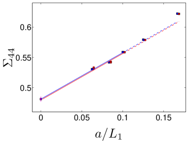
Refer to caption Refer to caption
Figure 11: Effect of tree level improvement on Σ44subscriptΣ44\Sigma_{44} for (θ1,θ2)=(0.5,1)subscript𝜃1subscript𝜃20.51(\theta_{1},\theta_{2})=(0.5,1). The conventions are the same as in fig 4.

We provide the tree-level improvement coefficients under
http://www-zeuthen.desy.de/alpha/public_tables/.

References

  • [1] E. Eichten and B. Hill, An effective field theory for the calculation of matrix elements involving heavy quarks, Phys. Lett. B234 (1990) 511.
  • [2] N. Isgur and M. B. Wise, Weak decays in the static quark approximation, Phys. Lett. B232 (1989) 113–117.
  • [3] H. Georgi, An effective field theory for heavy quarks at low energies, Phys. Lett. B240 (1990) 447–450.
  • [4] E. Eichten and B. Hill, Static effective field theory: 1/m corrections, Phys. Lett. B243 (1990) 427–431.
  • [5] B. Grinstein, The static quark effective theory, Nucl. Phys. B339 (1990) 253–268.
  • [6] ALPHA Collaboration, J. Heitger and J. Wennekers, Effective heavy-light meson energies in small-volume quenched QCD, JHEP 02 (2004) 064, [hep-lat/0312016].
  • [7] M. Della Morte, P. Fritzsch, J. Heitger, and R. Sommer, Non-perturbative quark mass dependence in the heavy-light sector of two-flavour QCD, PoS LATTICE2008 (2008) 226, [0810.3166].
  • [8] M. Antonelli et. al., Flavor Physics in the Quark Sector, 0907.5386.
  • [9] ALPHA Collaboration, M. Kurth and R. Sommer, Heavy quark effective theory at one-loop order: An explicit example, Nucl. Phys. B623 (2002) 271–286, [hep-lat/0108018].
  • [10] J. Heitger and A. Jüttner, Lattice cutoff effects for FDssubscript𝐹subscript𝐷𝑠F_{D_{s}} with improved Wilson fermions - a final lesson from the quenched case, JHEP 05 (2009) 101, [0812.2200].
  • [11] A. S. Kronfeld, Heavy quarks and lattice qcd, Nucl. Phys. Proc. Suppl. 129 (2004) 46–59, [hep-lat/0310063].
  • [12] N. Garron, Status of heavy quark physics from the lattice, Nucl. Phys. Proc. Suppl. 174 (2007) 193–198, [hep-ph/0612155].
  • [13] M. Della Morte, Standard Model parameters and heavy quarks on the lattice, PoS LAT2007 (2007) 008, [0711.3160].
  • [14] E. Gamiz, Heavy flavour phenomenology from lattice QCD, 0811.4146.
  • [15] C. Aubin, Lattice studies of hadrons with heavy flavors, 0909.2686.
  • [16] ALPHA Collaboration, J. Heitger and R. Sommer, Non-perturbative heavy quark effective theory, JHEP 02 (2004) 022, [hep-lat/0310035].
  • [17] ALPHA Collaboration, M. Della Morte, N. Garron, M. Papinutto, and R. Sommer, Heavy quark effective theory computation of the mass of the bottom quark, JHEP 01 (2007) 007, [hep-ph/0609294].
  • [18] M. Della Morte, A. Shindler, and R. Sommer, On lattice actions for static quarks, JHEP 08 (2005) 051, [hep-lat/0506008].
  • [19] ALPHA Collaboration, M. Kurth and R. Sommer, Renormalization and O(a𝑎a)-improvement of the static axial current, Nucl. Phys. B597 (2001) 488–518, [hep-lat/0007002].
  • [20] M. Bochicchio, L. Maiani, G. Martinelli, G. C. Rossi, and M. Testa, Chiral symmetry on the lattice with Wilson fermions, Nucl. Phys. B262 (1985) 331.
  • [21] M. Lüscher, S. Sint, R. Sommer, and H. Wittig, Nonperturbative determination of the axial current normalization constant in O(a𝑎a) improved lattice QCD, Nucl. Phys. B491 (1997) 344–364, [hep-lat/9611015].
  • [22] B. Blossier, M. Della Morte, G. von Hippel, T. Mendes, and R. Sommer, On the generalized eigenvalue method for energies and matrix elements in lattice field theory, JHEP 04 (2009) 094, [0902.1265].
  • [23] ALPHA Collaboration, J. Heitger, M. Kurth, and R. Sommer, Non-perturbative renormalization of the static axial current in quenched qcd, Nucl. Phys. B669 (2003) 173–206, [hep-lat/0302019].
  • [24] ALPHA Collaboration, J. Heitger, A. Jüttner, R. Sommer, and J. Wennekers, Non-perturbative tests of heavy quark effective theory, JHEP 11 (2004) 048, [hep-ph/0407227].
  • [25] K. G. Chetyrkin and A. G. Grozin, Three-loop anomalous dimension of the heavy-light quark current in hqet, hep-ph/0303113.
  • [26] S. Bekavac et. al., Matching QCD and HQET heavy-light currents at three loops, 0911.3356.
  • [27] M. Della Morte, P. Fritzsch, and J. Heitger, Non-perturbative renormalization of the static axial current in two-flavour QCD, JHEP 02 (2007) 079, [hep-lat/0611036].
  • [28] M. Della Morte et. al., Heavy-strange meson decay constants in the continuum limit of quenched QCD, JHEP 02 (2008) 078, [0710.2201].
  • [29] M. Lüscher, P. Weisz, and U. Wolff, A numerical method to compute the running coupling in asymptotically free theories, Nucl. Phys. B359 (1991) 221–243.
  • [30] A. Grimbach, D. Guazzini, F. Knechtli, and F. Palombi, O(a) improvement of the HYP static axial and vector currents at one-loop order of perturbation theory, JHEP 03 (2008) 039, [0802.0862].
  • [31] M. Lüscher, S. Sint, R. Sommer, P. Weisz, and U. Wolff, Non-perturbative O(a𝑎a) improvement of lattice QCD, Nucl. Phys. B491 (1997) 323–343, [hep-lat/9609035].
  • [32] A. Hasenfratz and F. Knechtli, Flavor symmetry and the static potential with hypercubic blocking, Phys. Rev. D64 (2001) 034504, [http://arXiv.org/abs/hep-lat/0103029].
  • [33] B. Blossier et. al., Spectroscopy and Decay Constants from Nonperturbative HQET at Order 1/m, 0911.1568.
  • [34] M. Lüscher, R. Narayanan, P. Weisz, and U. Wolff, The Schrödinger functional: A renormalizable probe for nonabelian gauge theories, Nucl. Phys. B384 (1992) 168–228, [hep-lat/9207009].
  • [35] S. Sint, On the Schrödinger functional in QCD, Nucl. Phys. B421 (1994) 135–158, [hep-lat/9312079].
  • [36] ALPHA Collaboration, G. de Divitiis et. al., Universality and the approach to the continuum limit in lattice gauge theory, Nucl. Phys. B437 (1995) 447–470, [hep-lat/9411017].
  • [37] ALPHA Collaboration, A. Bode, P. Weisz, and U. Wolff, Two loop computation of the Schrödinger functional in lattice QCD, Nucl. Phys. B576 (2000) 517–539, [Erratum-ibid.B600:453,2001, Erratum-ibid.B608:481,2001, hep-lat/9911018].
  • [38] ALPHA Collaboration, M. Della Morte et. al., Computation of the strong coupling in QCD with two dynamical flavours, Nucl. Phys. B713 (2005) 378–406, [hep-lat/0411025].
  • [39] P. Hasenfratz, The theoretical background and properties of perfect actions, hep-lat/9803027.
  • [40] S. Sint and P. Weisz, Further results on O(a𝑎a) improved lattice QCD to one loop order of perturbation theory, Nucl. Phys. B502 (1997) 251, [hep-lat/9704001].
  • [41] M. Lüscher, S. Sint, R. Sommer, and P. Weisz, Chiral symmetry and O(a𝑎a) improvement in lattice QCD, Nucl. Phys. B478 (1996) 365–400, [hep-lat/9605038].