On Estimation of Fully Entangled Fraction

Rui-Juan Gu ¹, Ming Li², Shao-Ming Fei¹ and Xianqing Li-Jost^3,4

$~{}^{1}$ School of Mathematical Sciences, Capital Normal University, 100048 Beijing

$~{}^{2}$ College of Mathematics and Computational Science, China University of Petroleum, 257061 Dongying

$~{}^{3}$ Max-Planck-Institute for Mathematics in the Sciences, 04103 Leipzig

$~{}^{4}$ Department of Mathematics, Hainan Normal University, 571158 Haikou

Abstract

We study the fully entangled fraction (FEF) of arbitrary mixed states. New upper bounds of FEF are derived. These upper bounds make complements on the estimation of the value of FEF. For weakly mixed quantum states, an upper bound is shown to be very tight to the exact value of FEF.

PACS numbers: 03.67.-a, 02.20.Hj, 03.65.-w

Quantum entanglement plays crucial roles in quantum information processing such as quantum computation nielsen ; di , quantum teleportation teleportation ; teleportation1 , dense coding dense , quantum cryptographic schemes schemes , entanglement swapping swapping and remote states preparation (RSP) RSP1 ; RSP2 ; RSP4 . For instance in terms of a classical communication channel and a quantum resource (a nonlocal entangled state like an EPR-pair of particles), the teleportation protocol gives ways to transmit an unknown quantum state from a sender to a receiver that are spatially separated. When the sender and receiver share a maximally entangled pure state, the state can be perfectly teleported. However when the shared entangled state is an arbitrary mixed state $\rho$, then the optimal fidelity of teleportation is given by teleportation1 ; yang ,

$$f(\rho)=\frac{d{\cal{F}}(\rho)}{d+1}+\frac{1}{d+1},$$ (1)

which solely depends on the fully entangled fraction (FEF) ${\cal{F}}(\rho)$ of $\rho$. Detailed discussion about FEF can be found in Ref. intr .

In fact the quantity FEF plays essential roles in many other quantum information processing such as dense coding, entanglement swapping and quantum cryptography (Bell inequalities). Thus it is very important to compute the FEF of general quantum states. Unfortunately, precise formula of FEF has been only obtained for two qubits systems grondalski . For high dimensional systems, it becomes quite difficult to derive an analytic formula for FEF. In li we have derived an upper bound of FEF to give an estimation of the value of FEF. In this paper, we derive more tight upper bounds for FEF. These bounds make complements on the estimation of FEF.

Let ${\mathcal{H}}$ be a $d$-dimensional complex vector space with computational basis $|i\rangle$, $i=1,...,d$. The fully entangled fraction of a density matrix $\rho\in{\mathcal{H}}\otimes{\mathcal{H}}$ is defined by

$${\mathcal{F}}(\rho)=\max_{\phi\in\epsilon}\langle\phi|\rho|\phi\rangle,$$ (2)

where $\epsilon$ denotes the set of $d\times d$-dimensional maximally entangled pure states. (2) can be also alternatively expressed as

$${\mathcal{F}}(\rho)=\max_{U}\langle\psi_{+}|(I\otimes U^{{\dagger}})\rho(I\otimes U)|\psi_{+}\rangle,$$ (3)

where the maximization is taken over all unitary transformations $U$, $|\psi_{+}\rangle=\frac{1}{\sqrt{d}}\sum\limits_{i=1}^{d}|ii\rangle$ is the maximally entangled state and $I$ is the corresponding identity matrix.

Let $h$ and $g$ be $d\times d$ matrices such that $h|j\rangle=|(j+1)\mod d\rangle,$g$|j\rangle=\omega^{j}|j\rangle$, with $\omega=exp\{\frac{-2i\pi}{d}\}$. We can introduce $d^{2}$ linear-independent $d\times d$-matrices $U_{st}=h^{t}g^{s}$, which satisfy

$$U_{st}U_{s^{\prime}t^{\prime}}=\omega^{st^{\prime}-ts^{\prime}}U_{s^{\prime}t^{\prime}}U_{st},{\rm Tr}(U_{st})=d\delta_{s0}\delta_{t0}.$$ (4)

$\left\{U_{st}\right\}$ also satisfy the condition for bases of unitary operators in the sense of Wer00 , i.e.

$$\left\{\begin{array}[]{l}tr\left(U_{st}U^{+}_{s^{\prime}t^{\prime}}\right)=d\delta_{tt^{\prime}}\delta_{ss^{\prime}},\\ U_{st}U_{st}^{+}=I.\end{array}\right.$$ (5)

$\left\{U_{st}\right\}$ form a complete basis of $d\times d$-matrices, namely, for any $d\times d$ matrix $W$, $W$ can be expressed as

$$W=\frac{1}{d}\sum_{s,t}tr(U_{st}^{+}W)U_{st}.$$ (6)

From $\{U_{st}\}$, we can introduce the generalized Bell-states,

$$|\Phi_{st}\rangle=(I\otimes U^{*}_{st})|\psi_{+}\rangle=\frac{1}{\sqrt{d}}\sum_{i,j}(U_{st})^{*}_{ij}|ij\rangle,{\rm and}~{}|\Phi_{00}\rangle=|\psi_{+}\rangle,$$ (7)

$|\Phi_{st}\rangle$ are all maximally entangled states and form a complete orthogonal normalized basis of ${\mathcal{H}}\otimes{\mathcal{H}}$.

Theorem 1: For any quantum state $\rho\in{\mathcal{H}}\otimes{\mathcal{H}}$, the fully entangled fraction defined in $(\ref{def})$ and $(\ref{def1})$ fulfills the following inequality:

$${\mathcal{F}}(\rho)\leq\max_{j}\{\lambda_{j}\},$$ (8)

where $\lambda_{j}$s are the eigenvalues of the real part of the matrix $M=\left(\begin{array}[]{cc}T&iT\\ -iT&T\\ \end{array}\right)$, $T$ is a $d^{2}\times d^{2}$ matrix with entries $T_{n,m}=\langle\Phi_{n}|\rho|\Phi_{m}\rangle$ and $\Phi_{j}$ is the maximally entangled basis states defined in $(\ref{bellbas})$.

Proof: From $(\ref{3e})$, any $d\times d$ unitary matrix $U$ can be represented as $U=\sum_{k=1}^{d^{2}}z_{k}U_{k},$ where $z_{k}=\frac{1}{d}{\rm Tr}(U_{k}^{{\dagger}}U)$, $U_{k}$ are the unitary matrices defined in (4). Define

$$x_{l}=\left\{\begin{array}[]{l}{\rm Re}[z_{l}],1\leq l\leq d^{2};\\ {\rm Im}[z_{l}],d^{2}<l\leq 2d^{2}\end{array}\right.~{}{\rm{and\quad}}U^{{}^{\prime}}_{l}=\left\{\begin{array}[]{l}U_{l},1\leq l\leq d^{2};\\ i*U_{l},d^{2}<l\leq 2d^{2}.\end{array}\right.$$ (9)

Then the unitary matrix $U$ can be rewritten as $U=\sum_{k=1}^{2d^{2}}x_{k}U^{{}^{\prime}}_{k}$. The necessary unitary condition of $U$, ${\rm{Tr}}(UU^{{\dagger}})=d$, requires that $\sum_{k}x_{k}^{2}=1$. Set

$$F(\rho)\equiv\langle\psi_{+}|(I\otimes U^{{\dagger}})\rho(I\otimes U)|\psi_{+}\rangle=\sum_{m,n=1}^{2d^{2}}x_{m}x_{n}M_{mn},$$ (10)

where $M_{mn}$ is the entry of the matrix $M$ defined in theorem. From the hermiticity of $\rho$ it is easily verified that

$$M_{mn}^{*}=M_{nm}.$$ (11)

To maximize $F(\rho)$ under constraints we get the following equation

$$\frac{\partial}{\partial x_{k}}\{F(\rho)+\lambda(\sum_{l}x_{l}^{2}-1)\}=0.$$ (12)

Taking into account $(\ref{hhh})$ we obtain an eigenvalue equation,

$$\sum_{n=1}^{2d^{2}}{\rm{Re}}[M_{k,n}]x_{n}=-\lambda x_{k}.$$ (13)

Therefore

$${\mathcal{F}}(\rho)=\max_{U}F(\rho)\leq\max_{j}\{\eta_{j}\},$$ (14)

where $\eta_{j}=-\lambda_{j}$ is the corresponding eigenvalues of the real part of matrix $M$. $\hfill\Box$

The upper bound derived in li says that for any $\rho\in{\mathcal{H}}\otimes{\mathcal{H}}$, the fully entangled fraction ${\mathcal{F}}(\rho)$ satisfies

$${\mathcal{F}}(\rho)\leq\frac{1}{d^{2}}+4||N^{T}(\rho)N(P_{+})||_{KF},$$ (15)

where $N(\rho)$ denotes the correlation matrix with entries $n_{ij}(\rho)$ given in the expression of $\rho$

$$\rho=\frac{1}{d^{2}}I\otimes I+\frac{1}{d}\sum\limits_{i=1}^{d^{2}-1}r_{i}(\rho)\lambda_{i}\otimes I+\frac{1}{d}\sum\limits_{j=1}^{d^{2}-1}s_{j}(\rho)I\otimes\lambda_{j}+\sum\limits_{i,j=1}^{d^{2}-1}n_{ij}(\rho)\lambda_{i}\otimes\lambda_{j},$$ (16)

$\lambda_{i}$, $i=1,...,d^{2}-1$, are the generators of the $SU(d)$ algebra with $Tr\{\lambda_{i}\lambda_{j}\}=2\delta_{ij}$, $r_{i}(\rho)=\frac{1}{2}Tr\{\rho\lambda_{i}(1)\otimes I\}$, $s_{j}(\rho)=\frac{1}{2}Tr\{\rho I\otimes\lambda_{j}(2)\}$, $n_{ij}(\rho)=\frac{1}{4}Tr\{\rho\lambda_{i}(1)\otimes\lambda_{j}(2)\}$, $P_{+}$ stands for the projection operator to $|\psi_{+}\rangle$, $N(P_{+})$ is similarly defined to $N(\rho)$, $N^{T}$ stands for the transpose of $N$, $||N||_{KF}=Tr\sqrt{NN^{{\dagger}}}$ is the Ky Fan norm of $N$. This upper bound was used to improve the distillation protocol proposed in gdp . Here we show that the upper bound in $(\ref{newfef})$ is different from that in $(\ref{oub})$ by an example.

Example 1: We consider the bound entangled state ho232

$$\rho(a)=\frac{1}{8a+1}\left(\begin{array}[]{ccccccccc}a&0&0&0&a&0&0&0&a\\ 0&a&0&0&0&0&0&0&0\\ 0&0&a&0&0&0&0&0&0\\ 0&0&0&a&0&0&0&0&0\\ a&0&0&0&a&0&0&0&a\\ 0&0&0&0&0&a&0&0&0\\ 0&0&0&0&0&0&\frac{1+a}{2}&0&\frac{\sqrt{1-a^{2}}}{2}\\ 0&0&0&0&0&0&0&a&0\\ a&0&0&0&a&0&\frac{\sqrt{1-a^{2}}}{2}&0&\frac{1+a}{2}\\ \end{array}\right).$$ (17)

From Fig. 1 we see that for $0\leq a<0.572$, the upper bound in $(\ref{newfef})$ is larger than that in $(\ref{oub})$. But for $0.572<a<1$ the upper bound in $(\ref{newfef})$ is always lower than that in $(\ref{oub})$, i.e. the upper bound $(\ref{newfef})$ is tighter than $(\ref{oub})$ in this case.

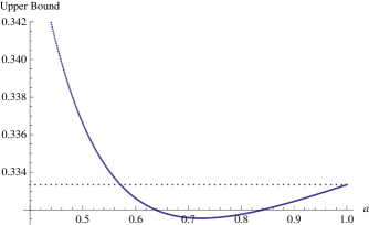
Figure 1: Upper bound of ${\mathcal{F}}(\rho)$ from (8) (solid line) and upper bound from $(\ref{oub})$ (dashed line).

By using the operator norm, we have further

Observation: For any $\rho\in{\mathcal{H}}\otimes{\mathcal{H}}$, the fully entangled fraction ${\mathcal{F}}(\rho)$ satisfies

$${\mathcal{F}}(\rho)\leq\max_{i}\{\lambda_{i}\}$$ (18)

where $\lambda_{i}$s are the eigenvalues of $\rho$.

Proof: For any quantum state $\rho$ and unitary $U$, we have

$$\langle\psi_{+}|(I\otimes U^{{\dagger}})\rho(I\otimes U)|\psi_{+}\rangle\leq\|\langle\psi_{+}|\|\|(I\otimes U^{\dagger})\rho(I\otimes U)|\psi_{+}\rangle\|$$

$$\leq\|(I\otimes U^{\dagger})\rho(I\otimes U)\|\||\psi_{+}\rangle\|^{2}=\|\rho\|\||\psi_{+}\rangle\|^{2}=\|\rho\|,$$ (19)

where $\|\rho\|$ stands for the operator norm, $\|\rho\|=sup(\|\rho|x\rangle\|:\||x\rangle\|=1)$, $\||x\rangle\|=\sqrt{\langle x|x\rangle}$. We have used the Cauchy-Schwarz inequality to obtain the first inequality. The second inequality is due to the basic property of operator norm. The followed equality follows from the fact that unitary transformation does not change the operator norm.

From conway $\|\rho\|$ is an eigenvalue of $\rho$, actually, it is the maximal eigenvalue of $\rho$, i.e. $\|\rho\|=\max_{i}\{\lambda_{i}\}$ where $\lambda_{i}$s are the eigenvalues of $\rho$, which ends the proof. $\hfill\Box$

This bound can give rise to further

Corollary: Let $|\psi\rangle=\sum_{ij}a_{ij}|ij\rangle$ with $|||\psi\rangle||=1$ be the normalized eigenvector of $\rho$ with respect to the maximal eigenvalue $\lambda_{max}$. If the matrix $A$ with elements $A_{ij}=\sqrt{d}a_{ij}$ are unitary, the upper bound derived in $(\ref{22})$ becomes the exact value of FEF.

Proof: A simple computation shows that

$${\mathcal{F}}(\rho) \leq\lambda_{max}=\langle\psi|\rho|\psi\rangle=\frac{1}{d}\sum_{ij,kl}\sqrt{d}a_{ij}^{*}\langle ij|\rho\sqrt{d}a_{kl}|kl\rangle$$

$$=\sum_{i,k}\frac{1}{d}\langle ii|I\otimes A^{{\dagger}}\rho I\otimes A|kk\rangle=\langle\psi_{+}|I\otimes A^{{\dagger}}\rho I\otimes A|\psi_{+}\rangle\leq{\mathcal{F}}(\rho).$$

Thus we have ${\mathcal{F}}(\rho)=\lambda_{max}$. $\hfill\Box$

According to the corollary, we can find out when the upper bound derived in theorem 2 becomes the exact value of FEF.

Example 2: Consider the $3\otimes 3$ state prl1056

$$\rho=\frac{2}{7}|\psi_{+}\rangle\langle\psi_{+}|+\frac{\alpha}{7}\sigma_{+}+\frac{5-\alpha}{7}\sigma_{-},$$ (20)

where $\sigma_{+}=\frac{1}{3}(|01\rangle\langle 01|+|12\rangle\langle 12|+|20\rangle\langle 20|),\sigma_{-}=\frac{1}{3}(|10\rangle\langle 10|+|21\rangle\langle 21|+|02\rangle\langle 02|)$. $\rho$ is entangled when $3<\alpha\leq 5.$ The maximal eigenvalue of $\rho$ is $\frac{2}{7}$, with the corresponding normalized eigenvector $\{\frac{1}{\sqrt{3}},0,0,0,\frac{1}{\sqrt{3}},0,0,0,\frac{1}{\sqrt{3}}\}$. The matrix $A$ related to this eigenvector is just the $3\times 3$ identity matrix which is obviously unitary. Thus we have for the state $(\ref{rr})$, ${\mathcal{F}}(\rho)=\frac{2}{7}$.

The following upper bound of FEF gives a very tight estimation of FEF for weakly mixed quantum states.

Theorem 2: For any bipartite quantum state $\rho\in{\mathcal{H}}\otimes{\mathcal{H}}$, the following inequality holds:

$${\mathcal{F}}(\rho)\leq\frac{1}{d}({\rm{Tr}}\sqrt{\rho_{A}})^{2},$$ (21)

where $\rho_{A}$ is the reduced matrix of $\rho$.

Proof: Note that the FEF for pure state $|\psi\rangle$ is given by gdp

$${\mathcal{F}}(|\psi\rangle)=\frac{1}{d}({\rm{Tr}}\sqrt{\rho_{A}^{|\psi\rangle}})^{2},$$ (22)

where $\rho_{A}^{|\psi\rangle}$ is the reduced matrix of $|\psi\rangle\langle\psi|$.

For mixed state $\rho=\sum_{i}p_{i}\rho^{i}$, we have

$${\mathcal{F}}(\rho) = \max_{U}\langle\psi_{+}|(I\otimes U^{{\dagger}})\rho(I\otimes U)|\psi_{+}\rangle$$ (23)

$$\leq \sum_{i}p_{i}\max_{U}\langle\psi_{+}|(I\otimes U^{{\dagger}})\rho^{i}(I\otimes U)|\psi_{+}\rangle$$

$$= \frac{1}{d}\sum_{i}p_{i}({\rm{Tr}}\sqrt{\rho_{A}^{i}})^{2}=\frac{1}{d}\sum_{i}({\rm{Tr}}\sqrt{p_{i}\rho_{A}^{i}})^{2}.$$

Let $\lambda_{ij}$ be the real and nonnegative eigenvalues of the matrix $p_{i}\rho_{A}^{i}$. Recall that for any function $F=\sum_{i}(\sum_{j}x_{ij}^{2})^{\frac{1}{2}}$ subjected to the constraints $z_{j}=\sum_{i}x_{ij}$ with $x_{ij}$ being real and nonnegative, the inequality $\sum_{j}z_{j}^{2}\leq F^{2}$ holds. It follows that

$${\mathcal{F}}(\rho)\leq\frac{1}{d}\sum_{i}\left(\sum_{j}\sqrt{\lambda_{ij}}\right)^{2}\leq\frac{1}{d}\left(\sum_{j}\sqrt{\sum_{i}\lambda_{ij}}\right)^{2}=\frac{1}{d}({\rm{Tr}}\sqrt{\rho_{A}})^{2},$$ (24)

which ends the proof. $\hfill\Box$

We now give an example to show that when the quantum state is weakly mixed, theorem 3 will be a very good estimation for the FEF.

Example 3: Consider the following $3\otimes 3$ mixed state: $\rho=\frac{1-p}{9}I_{9}+p|\psi\rangle\langle\psi|$, where $|\psi\rangle=\sqrt{\frac{x^{2}+2}{3}}\{x,0,0,0,1,0,0,0,1\}$ is a pure state with one parameter $x$. To show the effectiveness of (21), we compare it with the single fraction of entanglement $F_{s}=\langle\psi_{+}|\rho|\psi_{+}\rangle$. As seen from the Fig. 2, for weakly mixed states (with larger parameter $p$), the bound provides excellent estimation of the FEF.

Figure 2: Upper bound of ${\mathcal{F}}(\rho)$ from (21) (solid line) and single fraction of entanglement $F_{s}$

We have studied the fully entangled fraction that has tight relations with many quantum information processing. New upper bounds for FEF have been derived. They make complements on estimation of the value of FEF. The conditions for the bounds to be exact or to be more tight have been analyzed. These bounds provide a better estimation of FEF and can be use in related information processing, e.g. to detect the entanglement of the non-local source used in quantum teleportation. Our results also give rise to good estimations for the conditional min-entropy $H_{min}(A|B)$ and $q_{corr(A|B)}$ according to relation in 0807.1338 .

Acknowledgments  This work is supported by NSFC 10675086, 10875081, 10871227, KZ200810028013 and NKBRPC(2004CB318000).

References

• (1) M.A. Nielsen, I.L. Chuang, Quantum Computation and Quantum Information. Cambridge: Cambridge University Press, (2000).
• (2) See, for example, D.P. Di Vincenzo, Science 270,255(1995)
• (3) C.H. Bennett, G. Brassard, C. CrΓ©peau, R. Jozsa, A. Peres and W.K. Wootters, Phys. Rev. Lett. 70, 1895 (1993);
S. Albeverio and S.M. Fei, Phys.Lett. A 276, 8(2000);
G.M. D’Ariano, P. Lo Presti and M.F. Sacchi, Phys. Lett. A 272, 32(2000).
• (4) S. Albeverio, S.M. Fei and W.L. Yang, Phys. Rev. A 66, 012301(2002).
• (5) C.H. Bennett and S.J. Wiesner, Phys. Rev. Lett. 69, 2881(1992).
• (6) A. Ekert, Phys. Rev. Lett. 67, 661(1991);
D. Deutsch, A. Ekert, P. Rozas, C. Macchicavello, S. Popescu and A. Sanpera, Phys. Rev. Lett. 77, 2818(1996);
C.A. Fuchs, N. Gisin, R.B. Griffiths, C.S. Niu and A. Peres, Phys. Rev. A 56, 1163(1997).
• (7) M.Ε»ukowski, A. Zeilinger, M.A. Horne and A.K. Ekert, Phys. Rev. Lett. 71, 4287(1993);
S. Bose, V. Vedral and P.L. Knight, Phys. Rev. A 57, 822(1998); 60, 194(1999);
B.S. Shi, Y.K. Jiang, G.C. Guo, Phys. Rev. A 62, 054301(2000);
L. Hardy and D.D. Song, Phys. Rev. A 62, 052315(2000).
• (8) C.H. Bennett, D.P. DiVincenzo, P.W. Shor, J.A. Smolin, B.M. Terhal and W.K. Wootter, Phys. Rev. Lett. 87, 077902(2001).
• (9) B.S. Shi and A. Tomita, J. Opt. B: Quant. Semiclass. Opt. 4, 380(2002); J.M. Liu and Y.Z. Wang, Chinese Phys. 13, 147(2004).
• (10) M.Y. Ye, Y.S. Zhang and G.C. Guo, Phys. Rev. A 69, 022310(2004).
• (11) M. Horodecki, P. Horodecki and R. Horodecki, Phys. Rev. A, 60, 1888(1999).
• (12) C. H. Bennett, D. P. DiVincenzo, J. A. Smolin, and W. K. Wooters, et. al., Phys. Rev. A 54, 3824 (1996);
M. Horodecki, P. Horodecki, and R. Horodecki, Phys. Rev. A 60, 1888 (1999);
C. S. Yu, X. X. Yi, and H. S. Song, Phys. Rev. A 78, 062330 (2008).
• (13) J. Grondalski, D. M. Etlinger and D. F. V. James, Phys. Lett. A 300, 573(2002).
• (14) M. Li, S.M. Fei and Z.X. Wang, Phys. Rev. A, 78, 032332(2008).
• (15) R.F. Werner, J. Phys. A, 34, 7081-7094(2001).
• (16) M. Horodecki and P. Horodecki, Phys. Rev. A, 59, 4206(2002).
• (17) P. Horodecki, Phys. Lett. A 232, 333(1997).
• (18) John B. Conway, ”A Course in Functional Analysis” Springer-Verlag,(1985) Page 48.
• (19) P. Horodecki, M. Horodecki and R. Horodecki, Phys. Rev. L. 82, 1056(1999).
• (20) T. Konrad, F. De Melo, M. Tiersch, C. Kasztelan, A. Aragao, and A. Buchleitner, Nature(London), 4, 99(2008).
• (21) R. Koenig, R. Renner, C. Schaffner, The operational meaning of min- and max-entropy, arXiv: 0807.1338(2008).