January 2010

Giant Holes

Nick Dorey and Manuel Losi
DAMTP, Centre for Mathematical Sciences
University of Cambridge, Wilberforce Road
Cambridge CB3 0WA, UK
Abstract

We study the semiclassical spectrum of excitations around a long spinning string in $AdS_{3}$. In addition to the usual small fluctuations, we find the spectrum contains a branch of solitonic excitations of finite energy. We determine the dispersion relation for these excitations. This has a relativistic form at low energies but also matches the dispersion relation for the “holes” of the dual gauge theory spin chain at high energies. The low-energy behaviour is consistent with the hypothesis that the solitonic excitations studied here are continuously related to the elementary excitations of the string.

The discovery of the integrability of the one-loop planar dilatation operator in ${\cal N}=4$ SUSY Yang-Mills [1, 2] and of the classical limit of the dual string theory on $AdS_{5}\times S^{5}$ [3] initiated a period of rapid progress in our understanding of the AdS/CFT correspondence. Recently this progress has culminated in a set of equations which are conjectured to describe the exact spectrum of both theories in the planar limit [4, 5, 6], for all values of the ’t Hooft coupling $\lambda=g^{2}_{YM}N$. So far most of this progress is based on our knowledge of the exact spectrum of excitations around the the one-half BPS chiral primary operator $\hat{O}_{\rm BPS}={\rm Tr}[Z^{J}]$ in the $J\rightarrow\infty$ large-volume limit and of the exact two body S-matrix for the scattering of these excitations [7, 8, 9, 10]. In particular, knowledge of this large-volume data is the starting point for the Y-system and Thermodynamic Bethe Ansatz approaches to the finite volume theory.

The BPS chiral primary operator described above corresponds to a point-like string orbiting the equator of the five-sphere in the dual geometry; also known as the BMN groundstate [11]. As recently emphasized in [13, 14], an alternative starting point or “ground-state” for quantization of the string is provided by the folded spinning string solution of Gubser, Klebanov and Polyakov [12]. This is the state of lowest dimension $\Delta$ with a single fixed spin, $S$, in $AdS_{5}$. In the $S\rightarrow\infty$ limit, the energy of this configuration is proportional to the cusp anomaly $\Gamma(\lambda)$ of the ${\cal N}=4$ theory and it is also a natural starting point for the connection to light-like Wilson loops and gluon scattering amplitudes discussed by Alday and Maldacena [14, 15]. As in the $J\rightarrow\infty$ limit of the BMN groundstate, the string effectively becomes infinitely long in this large spin limit. As the worldsheet theory is integrable we expect that excitations of finite energy around this ground-state will correspond to particles which undergo factorised scattering. The main purpose of this note is to study these excitations in semiclassical string theory and compare them with the corresponding states in the dual gauge theory.

In the following we will focus on excitations with energy of order $\sqrt{\lambda}$ which appear as classical solutions of the worldsheet theory. A large class of solutions of this type has been constructed in [16] using the inverse scattering method. We will show that a particular subset of these solutions correspond to local excitations of the GKP spinning string which make a finite contribution to the energy $E=\Delta-S$ and we will investigate the dynamics of these states. Our main result is an explicit expresion for the dispersion relation of these excitations. We find that the energy and momentum of the soliton are related as,

$$E_{\rm sol}(v) = \frac{\sqrt{\lambda}}{2\pi}\left[\frac{1}{2}\log\left(\frac{1+\sqrt{1-v^{2}}}{1-\sqrt{1-v^{2}}}\right)\,\,-\,\,\sqrt{1-v^{2}}\right]$$

$$P_{\rm sol}(v) = \frac{\sqrt{\lambda}}{2\pi}\left[\frac{\sqrt{1-v^{2}}}{v}\,\,-\,\,{\rm Tan}^{-1}\left(\frac{\sqrt{1-v^{2}}}{v}\right)\right]$$ (1)

where the branch of inverse tangent is chosen so that $-\pi/2\leq{\rm Tan}^{-1}x\leq+\pi/2$ for all real values of $x$. Here $E_{\rm sol}$ is the contribution of the soliton to the energy $E=\Delta-S$. The momentum $P_{\rm sol}$ is canonically conjugate to the position of the soliton on the string in coordinates where the total length of the string grows like $2\log S$ as $S\rightarrow\infty$. The parameter $v\leq 1$ is the velocity of the soliton in these coordinates.

The physical information in the above dispersion relation is the semiclassical spectrum of states associated with the excitation. As we describe below, this corresponds to the relation $E_{\rm sol}(P_{\rm sol})$, as determined by (1), supplemented with the large-$S$ quantization condition,

$$P_{\rm sol}\cdot\,2\log S \in 2\pi\,\,\mathbb{Z}$$

The resulting spectrum can also be obtained from a semiclassical quantization of the finite gap construction of [17]. A more complete analysis will appear in the forthcoming paper [18].

At low momentum ($v\simeq 1$), the dispersion relation takes the relativistic form,

$$E_{\rm sol} \simeq |P_{\rm sol}|\,\,+\,\,{\rm O}\left(P^{\frac{5}{3}}_{\rm sol}\right)$$

This is similar to the behaviour of the Giant Magnons [23] which appear as solitonic excitations of the BMN groundstate. In that case the onset of relativistic behaviour at low momenta allows the identification of Giant Magnons with the elementary excitations of the string. In the following we will argue that a similar phenomenon should also occur in this case. Away from low energy the dispersion relation is non-relativistic. Although the conformal gauge string action and Virasoro constraint respect worldsheet Lorentz invariance, this symmetry is broken by fixing the residual gauge symmetry and the non-relativistic dispersion relation of the soliton reflects this breaking.

The spinning folded string in $AdS_{3}$ is dual to a certain twist two operator in ${\cal N}=4$ SUSY Yang-Mills. Excitations around this operator correspond to holes in the rapidity distribution in the corresponding integrable spin chain [25, 26]. These holes have the characteristics of particles carrying conserved momenta and each such hole contributes a finite amount to the anomalous dimension of the operator. Taking our dispersion relation (1) in the limit of large momentum ($v<<1$) we find,

$$E_{\rm sol} = \frac{\sqrt{\lambda}}{2\pi}\,\log\,|P_{\rm sol}|\,\,+\,\,{\rm O}\left(P^{0}_{\rm sol}\right)$$ (2)

As we review below, this precisely matches the relevant dispersion relation for so-called “large” holes up to the by now familiar replacement of the prefactor ${\sqrt{\lambda}}/{2\pi}$ with the cusp anomalous dimension $\Gamma(\lambda)$. This is one of several examples where gauge theory and string theory quantities agree modulo this replacement in the limit of large spin. In view of this agreement we suggest that the string solitons studied in this paper deserve the name “Giant Holes”. The implied relation between holes and classical solitons is reminiscent of similar phenomena occuring in the case of the non-linear Schrodinger equation [20].

We will now review the contruction of explicit solutions of the string equations of motion in $AdS_{3}$ [21, 16]. We start by representing the target space as a 3-dimensional hyperboloid embedded in $\mathbb{R}^{2,2}$ defined by the following constraint:

$$X_{\mu}X^{\mu}=-X_{0}^{2}-X_{1}^{2}+X_{2}^{2}+X_{3}^{2}=-1$$ (3)

The $\sigma$-model action, in conformal gauge, is then defined in terms of the embedding coordinates $X_{\mu}$ as:

$$I=-\frac{\sqrt{\lambda}}{4\pi}\int d\sigma d\tau\left[G_{\mu\nu}\partial_{a}X^{\mu}\partial^{a}X^{\nu}+\Lambda\left(X_{\mu}X^{\mu}+1\right)\right]$$ (4)

where $\lambda$ is the t’Hooft coupling and $G_{\mu\nu}=\mathrm{diag}(-1,-1,1,1)$ is the flat metric on $\mathbb{R}^{2,2}$. As we consider string motion in $AdS_{3}$ only, the Virasoro constraint takes the form,

$$\partial_{\pm}X^{\mu}\partial_{\pm}X_{\mu}=0$$ (5)

The embedding coordinates defined in (3) are related to the standard global coordinates in $AdS_{3}$ via the complex combinations,

$$Z_{1} = X_{0}+iX_{1}=\cosh\rho\;e^{it}$$

$$Z_{2} = X_{2}+iX_{3}=\sinh\rho\;e^{i\phi}$$ (6)

where $t$ is global time and $\phi\sim\phi+2\pi$ is an angular coordinate. As mentioned above, we will refer to the Noether charge conjugate to translations of the global time $t$ as dimension $\Delta$. Angular momentum $S$ in $AdS_{3}$ is canonically conjugate to translations of $\phi$. In terms of the string coordinates we have,

$$\Delta = \frac{\sqrt{\lambda}}{2\pi}\int d\sigma\;\mathrm{Im}(\bar{Z}_{1}\partial_{\tau}Z_{1})$$ (7)

$$S = \frac{\sqrt{\lambda}}{2\pi}\int d\sigma\;\mathrm{Im}(\bar{Z}_{2}\partial_{\tau}Z_{2})$$ (8)

where the integrals are taken over the appropriate range of the worldsheet coordinate $\sigma$.

Pohlmeyer’s reduction procedure [19, 22] starts by defining a set of basis vectors $\{B_{\mu},X_{\mu},$ $\partial_{+}X_{\mu},\partial_{-}X_{\mu}\}$ on $\mathbb{R}^{2,2}$ where,

$$B_{\mu}=e^{-\alpha}\epsilon_{\mu\nu\rho\sigma}X^{\nu}\partial_{-}X^{\rho}\partial_{+}X^{\sigma}$$ (9)

with,

$$\alpha = \ln(-\partial_{+}X_{\mu}\partial_{-}X^{\mu})$$

We also define the quantitities,

$$u = B_{\mu}\partial_{+}^{2}X^{\mu}$$

$$v = B_{\mu}\partial_{-}^{2}X^{\mu}$$

By virtue of this definition, as well as the equation of motion and Virasoro constraint, the basis vectors are orthogonal and each vector is either null or normalised to unity. In particular we have,

$$B_{\mu}B^{\mu}=1\>,\qquad B_{\mu}X^{\mu}=B_{\mu}\partial_{+}X^{\mu}=B_{\mu}\partial_{-}X^{\mu}=0\>,$$ (10)

The string equations of motion and Virasoro constraint can then be transformed into equations for $\alpha$, $u$ and $v$. we find,

$$\partial_{+}\partial_{-}\alpha+e^{\alpha}+uve^{-\alpha}=0$$ (11)

together with the conditions $\partial_{-}u=\partial_{+}v=0$ which imply that we can set $u=u(\sigma^{+})$ and $v=v(\sigma^{-})$. Freedom to choose these functions of the left and right moving coordinates corresponds to the residual gauge invariance of the string left after fixing conformal gauge.

Now we introduce the following change of variable:

$$\hat{\alpha}=\alpha-\frac{1}{2}\ln|u||v|$$ (12)

and define rescaled spacetime coordinates $\hat{\sigma}^{\pm}$ so that,

$$\partial_{+}=\sqrt{2|u|}\hat{\partial}_{+}\>,\qquad\partial_{-}=\sqrt{2|v|}\hat{\partial}_{-}$$ (13)

Finally the remaining equation (11) takes the form,

$$\hat{\partial}_{+}\hat{\partial}_{-}\hat{\alpha}+\frac{1}{2}[e^{\hat{\alpha}}+\mathrm{sgn}(uv)e^{-\hat{\alpha}}]=0$$ (14)

which reduces to the sinh-Gordon equation when $uv<0$ and to the cosh-Gordon equation when $uv>0$. The strategy for finding string solutions is to start from known solutions of the sinh-Gordon equation, $\hat{\alpha}(\hat{\sigma}_{+},\hat{\sigma}_{-})$ and reconstruct the string coordinates by solving the auxiliary linear differential equations arising from the Lax formulation of the sinh-Gordon theory [16].

We now review the explicit solutions constructed in [16]. For convenience, from now on we will work in the worldsheet coordinates $\sigma$ and $\tau$, without introducing the transformation (13) (all the solutions we are going to consider have $u=2$, $v=-2$ and thus, in these coordinates, the sinh-Gordon equation becomes $\partial_{+}\partial_{-}\hat{\alpha}+4\sinh\hat{\alpha}=0$). The simplest case corresponds to the vacuum solution of the sinh-Gordon equation,

$$\hat{\alpha}_{0}=0\quad\mathrm{or}\quad\alpha_{0}=\ln 2$$ (15)

which yields the solution for the complex coordinates,

$$Z_{1} = X_{0}+iX_{1}=\cosh\rho\;e^{it}$$

$$Z_{2} = X_{2}+iX_{3}=\sinh\rho\;e^{i\phi}$$

which takes the form,

$$Z_{1} = e^{i\tau}\cosh\sigma$$

$$Z_{2} = e^{i\tau}\sinh\sigma$$ (16)

This corresponds to the infinite spin limit of the GKP [12] folded spinning string in $AdS_{3}$. For coordinate range $\sigma\in(-\infty,+\infty)$, it describes a straight line passing through the centre of $AdS_{3}$, extending up to the boundary, which rigidly rotates at constant angular velocity. One can glue two of these lines together in order to construct a folded closed string.

The energy and angular momentum of this solution are infinite. Hence we will regulate the problem by considering instead a closed string of finite length with folds at radial distance $\rho=\Lambda>>1$. Up to subleading corrections, this corresponds to the same solution but with the range of the worldsheet coordinate restricted as $-\Lambda\leq\sigma\leq+\Lambda$. We then find,

$$\Delta = \frac{\sqrt{\lambda}}{\pi}\int_{-\Lambda}^{\Lambda}d\sigma\cosh^{2}\sigma\,\,\,=\,\,\,\frac{\sqrt{\lambda}}{4\pi}\left(e^{2\Lambda}+4\Lambda-e^{-2\Lambda}\right)$$

$$S = \frac{\sqrt{\lambda}}{\pi}\int_{-\Lambda}^{\Lambda}d\sigma\sinh^{2}\sigma\,\,\,=\,\,\,\frac{\sqrt{\lambda}}{4\pi}\left(e^{2\Lambda}-4\Lambda-e^{-2\Lambda}\right)$$

Subtracting the regulated string energy and angular momentum we obtain the standard formula,

$$E_{0}\,\,=\,\,\Delta-S = \frac{\sqrt{\lambda}}{\pi}2\Lambda$$ (18)

$$= \frac{\sqrt{\lambda}}{\pi}\left[\log\left(\frac{\pi S}{\sqrt{\lambda}}\right)+2\log 2+O\left(\frac{\log S}{S}\right)\right]$$

In this paper we are interested in classical excitations of the long string solution which contribute a finite amount to the anomalous dimension $E=\Delta-S$. As the long string corresponds to the vacuum solution of the sinh-Gordon equation we expect that the configurations we seek should correspond to excitations of the sinh-Gordon vacuum. One such excitation corresponds to the small fluctuations of the sinh-Gordon field which carry energy of order one. Here we will focus instead on states which have energy $E\sim\sqrt{\lambda}$ and are visible as classical solutions of the string worldsheet theory. In fact, the sinh-Gordon equation has singular soliton solutions and these are natural candidates for the states we seek. The solution describing a single (anti-)soliton moving at velocity $v$ is given by,

$$\alpha_{s/\bar{s}}=\ln 2\pm\ln[\tanh^{2}(\gamma(\sigma-v\tau))]$$ (19)

where the positive and negative signs correspond to the choice of soliton ($s$) or anti-soliton ($\bar{s}$) respectively. Note that these configurations of the sinh-Gordon field $\hat{\alpha}$ are singular so it is not obvious that they should be thought of as fluctuations around the vacuum state. However, they do not necessarily lead to a singularity in the string solution. In fact, the relation,

$$-\partial_{+}X_{\mu}\partial_{-}X^{\mu} = \exp(\alpha)$$

shows that the singularity of the soliton solution simply corresponds to a zero of the quantity $\partial_{+}X_{\mu}\partial_{-}X^{\mu}$. Recalling the Virasoro constraint (5), we see that such a zero can occur at a cusp point of the string where derivatives $\partial_{\sigma}X_{\mu}$ vanish. The string solution is regular at such a point and worldsheet densities of conserved charges remain finite. As we see below, it seems that no such benign interpretation exists for the anti-soliton solution in the present context.

The sinh-Gordon equation is exactly integrable and, as a consequence, one can find exact solutions describing the scattering of any number of solitons and anti-solitons. For example, solutions describing the scattering of two solitons or two anti-solitons are:

$$\alpha_{ss,\bar{s}\bar{s}} = \ln 2\pm\ln\left[\frac{v\cosh X-\cosh T}{v\cosh X+\cosh T}\right]^{2}$$

where $X=2\gamma\sigma$, $T=2v\gamma\tau$ and $0<v<1$. The solution is given here in the centre of mass frame where the (anti-)solitons have equal and opposite velocities $\pm v$. As in the more conventional case of the sine-Gordon equation, the interaction between two solitons and between two anti-solitons is repulsive while that between a soliton and an anti-soliton is attractive and also gives rise to a classical boundstate or breather solution.

Following [16], one can construct string solutions corresponding to an arbitrary number of solitons and anti-solitons (and breathers) using the inverse scattering method. However we are primarily interested in solutions which correspond to local excitations of the vacuum configuration (16). In particular, we demand that the resulting string solutions asymptote to the vacuum solution (16) as $\sigma\rightarrow\pm\infty$ and also that the contribution of the excitation to the energy $E=\Delta-S$ is finite. In fact the only solution presented in [16] with the required property is the solution for the scattering of two solitons with non-zero velocities $\pm v$,

$$Z_{1}^{ss} = e^{i\tau}\frac{v\mathrm{ch}T\mathrm{ch}\sigma+\mathrm{ch}X\mathrm{ch}\sigma-\sqrt{1-v^{2}}\mathrm{sh}X\mathrm{sh}\sigma-i\sqrt{1-v^{2}}\mathrm{sh}T\mathrm{ch}\sigma}{\mathrm{ch}T+v\mathrm{ch}X}$$

$$Z_{2}^{ss} = e^{i\tau}\frac{v\mathrm{ch}T\mathrm{sh}\sigma+\mathrm{ch}X\mathrm{sh}\sigma-\sqrt{1-v^{2}}\mathrm{sh}X\mathrm{ch}\sigma-i\sqrt{1-v^{2}}\mathrm{sh}T\mathrm{sh}\sigma}{\mathrm{ch}T+v\mathrm{ch}X}$$

where $\mathrm{ch}X\equiv\cosh X$ and $\mathrm{sh}X\equiv\sinh X$ and $0<v<1$. Note that the global time $t$ and the worldsheet time $\tau$ are different for the above solution. Several plots of this solution at constant global time $t$ are shown in Fig. 1. This solution has two small spikes located at the positions of the two solitons, which start at the endpoints of the string, then approach each other until they scatter at the origin and then move away towards the endpoints. Interestingly the same solution plotted at constant worldsheet time $\tau$ has no cusps.

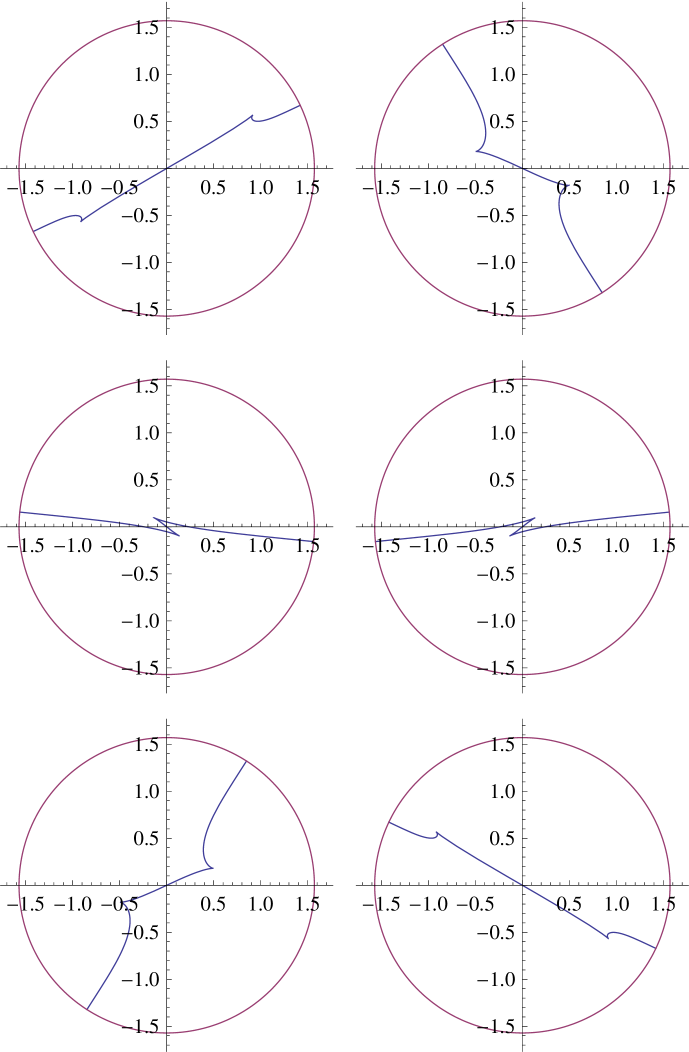
Figure 1: The 2-soliton solution at $t=-2.7,-1,-0.1,0.1,1,2.7$ (from left to right and top to bottom). At $t=0$ the string coincides with the horizontal axis.

The solution (LABEL:eq:2s_solution) has asymptotics,

$$Z_{1} \simeq \frac{1}{2}e^{\pm\sigma}\,e^{i\tau}\left(\frac{1-\sqrt{1-v^{2}}}{v}\right)$$

$$Z_{2} \simeq \pm\frac{1}{2}e^{\pm\sigma}\,e^{i\tau}\left(\frac{1-\sqrt{1-v^{2}}}{v}\right)$$ (21)

as $\sigma\rightarrow\pm\infty$ which indeed match those of the vacuum configuration (16) up to a finite shift in the radial coordinate $\rho$ which will be important in the following.

For the string solution corresponding to two anti-solitons, the denominators in (LABEL:eq:2s_solution) are replaced by $\mathrm{ch}T-v\mathrm{ch}X$ while in the solution for soliton-antisoliton scattering the relevant denominator is $\mathrm{sh}T\pm v\mathrm{sh}X$. The denominator for the breather solution then follows from analytic continuation to imaginary velocity $v=iw$. All of these denominators have zeros at finite values of $\sigma$ leading to poles in the corresponding solution which yield an infinite contribution to the energy. Hence, configurations involving anti-solitons do not seem to correspond to local excitations of the vacuum (16).

As for the vacuum solution, we will consider the solution (LABEL:eq:2s_solution) as one half of a long folded string extending to radial coordinate $\rho=\Lambda>>1$. The asymptotics (21) then imply we must restrict the spatial worldsheet coordinate to the range $-\tilde{\Lambda}\leq\sigma\leq+\tilde{\Lambda}$ with $\tilde{\Lambda}=\Lambda-\delta\Lambda$ where,

$$\delta\Lambda = \log\left(\frac{1-\sqrt{1-v^{2}}}{v}\right)\,\,\,=\,\,\,\frac{1}{2}\log\left(\frac{1-\sqrt{1-v^{2}}}{1+\sqrt{1-v^{2}}}\right)$$

In the second equality we have chosen the branch of the logarithm such that the expression is even under $v\rightarrow-v$. This is appropriate because the solution is invariant under the interchange of the two identical solitons. The shift $\delta\Lambda$ reflects the contribution of the excitations to the total length of the string. Note that it vanishes for $v=1$ where the two soliton solution simply reduces to the vacuum solution (16). On the other hand, the additional contribution diverges as $v\rightarrow 0$ indicating a change of the asymptotic behaviour of the string solution in this limit.

The resulting string energy $E=\Delta-S$ can be computed directly from the regulated solution. Relative to the vacuum solution, we replace one half of the closed string by the corresponding two soliton solution to get,

$$E = \frac{1}{2}E_{0}+\frac{\sqrt{\lambda}}{2\pi}\int_{-\tilde{\Lambda}}^{\tilde{\Lambda}}d\sigma\frac{1-3v^{2}+\cosh 2T+v^{2}\cosh 2X}{2(\cosh T+v\cosh X)^{2}}$$

$$= \frac{1}{2}E_{0}+\frac{\sqrt{\lambda}}{2\pi}\left[\sigma-\frac{v\sqrt{1-v^{2}}\sinh X}{\cosh T+v\cosh X}\right]_{-\tilde{\Lambda}}^{\tilde{\Lambda}}$$

$$= \frac{\sqrt{\lambda}}{2\pi}\left[2\Lambda+2\tilde{\Lambda}-2\sqrt{1-v^{2}}+O(e^{-2\gamma\Lambda})\right]$$

$$= E_{0}\,\,+\,\,2E_{\rm sol}(v)\,\,+\,\,O(e^{-2\gamma\Lambda})$$

where,

$$E_{\rm sol}(v) = \frac{\sqrt{\lambda}}{2\pi}\left[-\delta\Lambda\,\,-\,\,\sqrt{1-v^{2}}\right]$$ (22)

$$= \frac{\sqrt{\lambda}}{2\pi}\left[\frac{1}{2}\log\left(\frac{1+\sqrt{1-v^{2}}}{1-\sqrt{1-v^{2}}}\right)\,\,-\,\,\sqrt{1-v^{2}}\right]$$

is naturally interpreted as the energy of a single soliton of velocity $-1\leq v\leq+1$. Note that $E_{\rm sol}$ diverges as the soliton velocity $v$ goes to zero reflecting the divergent contribution to the length of the string mentioned above.

As the consitituent solitons of the two soliton scattering solution are well seperated at very early and late times, it is intuitively clear that string solutions corresponding to individual solitons with vacuum asymptotics must also exist. Indeed such solutions were also presented in [16] (see equations (4.25, 4.26)), but were found to have infinite energy. They also have different asymptotics to the vacuum configuration studied above. In fact this pathological behaviour arises because the solution (4.25, 4.26) of [16] corresponds to a single soliton with zero velocity and is related to the divergence of $E_{\rm sol}(v)$ as $v\rightarrow 0$ found above. A solution corresponding to a single soliton with non-zero velocity $v>0$ can be obtained by space and time translation of the two-soliton scattering solution so that one cusp is located near the origin and the other is sent to infinity. We construct such a solution in the Appendix and show that the solution indeed has vacuum asymptotics and energy $E_{0}+E_{\rm sol}$ as expected for a single soliton.

Having established the existence of excitations of finite energy we now want to determine their dispersion relation. In particular, as the cusps move along the string with velocity $v$ as measured in the spacelike worldsheet coordinate $\sigma$, we want to identify the conserved momentum $P_{\rm sol}(v)$ which is canonically conjugate to the position of the soliton in these coordinates. Here we will follow the same line of reasoning used for the case of Giant Magnons in [23]. Consider a configuration with $M$ cusps located at positions $\sigma=\sigma_{l}(\tau)$ in the worldsheet coordinate $\sigma$ introduced above, moving with velocities $v_{l}=d\sigma_{l}/d\tau$ for $l=1,\ldots,M$. The total energy of the configuration is,

$$E=E_{0}(S)\,\,+\,\,\sum_{l=1}^{M}\,E_{\rm sol}(v_{l})$$ (23)

The energy $E=\Delta-S$ is canonically conjugate to the global coordinate $\tilde{t}=(t+\phi)/2$ and we can define a canonical momentum $P_{l}$ for each soliton via Hamilton’s equation,

$$\frac{d{\sigma}_{l}}{d\tilde{t}} = \,\,\frac{\partial E}{\partial P_{l}}$$ (24)

An important subtlety is that the global time $\tilde{t}$ appearing in the above equation is not equal to the worldsheet time in the string solutions considered above. However they are equal in the vacuum solution (16) and, as each sinh-Gordon soliton is localised, we have $d\tilde{t}/d\tau\rightarrow 1$ exponentially fast away from the centre of each cusp. Thus the differential $\tilde{v}_{l}=d{\sigma}_{l}/d\tilde{t}$ appearing in (24) will be equal to the worldsheet velocity $v_{l}$ up to exponentially small corrections for almost all times. Making the replacement $\tilde{v}\rightarrow v$ in the Hamilton equation (24) for a single soliton moving at constant velocity $v$ we get,

$$v\,\,=\,\,\frac{dE_{\rm sol}}{dP_{\rm sol}} = \frac{dE_{\rm sol}}{dv}/\frac{dP_{\rm sol}}{dv}$$

or equivalently,

$$\frac{dP_{\rm sol}}{dv}\,\,=\,\,\frac{1}{v}\,\frac{dE_{\rm sol}}{dv} = -\frac{\sqrt{\lambda}}{2\pi}\frac{\sqrt{1-v^{2}}}{v^{2}}$$ (25)

where we used (22) in the second equality. As the soliton solutions considered above revert to the vacuum for $|v|=1$ we integrate (25) with boundary condition $P_{\rm sol}(\pm 1)=0$ to get,

$$P_{\rm sol}(v) = \frac{\sqrt{\lambda}}{2\pi}\left[\frac{\sqrt{1-v^{2}}}{v}\,\,-\,\,{\rm Tan}^{-1}\left(\frac{\sqrt{1-v^{2}}}{v}\right)\right]$$ (26)

Equations (22) and (26) constitute the dispersion relation of the soliton. Notice that the conserved momentum $P_{\rm sol}(v)$ is an odd function of the velocity $v$ by construction. Thus the total momentum of the two soliton solution considered above is zero. More generally we might expect that an $M$-soliton closed string solution should obey a level-matching condition of the form,

$$P = \sum_{l=1}^{M}\,P_{\rm sol}(v_{l})\,\,=\,\,0$$

As mentioned above, the situation is complicated by the fact that the folds at the end of the string themselves correspond to solitons with zero velocity which therefore yield two infinite contributions to the total momentum of opposite sign which can cancel up to a finite remainder. This consideration presumably allows for the existence of the one-soliton excitation of the folded string discussed in the Appendix.

As mentioned above, the physical content of the dispersion relation is contained in the semiclassical spectrum of excitations around the vacuum configuration. Classically the spin $S$ and soliton velocities $v_{l}$ are continuous parameters of the solution. In leading order semi-classical quantization $S$ is naturally quantized in integer units. In addition, the semiclassical wavefunction for a soliton of velocity $v$ takes the form,

$$\Psi(\sigma) = \exp\left(iP_{\rm sol}(v)\sigma\right)$$

The quantization condition for the soliton velocity comes from demanding that the wavefunction should be invariant under the shift $\sigma\rightarrow\sigma+2\Lambda+2\tilde{\Lambda}$ corresponding to a closed string of total length $L=2\Lambda+2\tilde{\Lambda}$. For our purpose the leading order behaviour $L\simeq 2\log(S)+{\rm O}(S^{0})$ is sufficient to find the leading-order quantization condition

$$P_{\rm sol}(v)\cdot 2\log S \in 2\pi\,\,\mathbb{Z}$$ (27)

Implementing these quantization conditions for each soliton contribution to the total energy (23) yields a definite prediction for the semiclassical spectrum. In a forthcoming paper we will reproduce this spectrum directly from the finite-gap formalism of [17].

It is interesting to compare our string theory results with the corresponding spectrum of excitations in the dual gauge theory. The dual to the GKP spinning string lies in the $SL(2)$ sector of the ${\cal N}=4$ theory consisting of operators of the form,

$$\hat{O} \sim {\rm Tr}_{N}\left[\,\mathcal{D}_{+}^{s_{1}}Z\,\mathcal{D}_{+}^{s_{2}}Z\,\ldots\,\mathcal{D}_{+}^{s_{J}}Z\,\right]$$ (28)

which have Lorentz spin $S=\sum_{l=1}^{J}\,\,s_{l}$ and twist $J$. Here $\mathcal{D}_{+}$ is a light-cone covariant derivative in Minkowski space. The one-loop anomalous dimensions of these operators are determined by the energy levels of an integrable ${\rm SL}(2,\mathbb{R})$ spin chain which are determined exactly by the Bethe ansatz. To formulate the Bethe ansatz one starts from the ferromagnetic vacuum of the spin chain which corresponds to the chiral primary $\hat{O}_{\rm BPS}={\rm Tr}_{N}Z^{J}$. Excitations around this groundstate corresponding to insertion of impurities $\mathcal{D}_{+}$, which carry one unit of spin $S$, and are known as magnons. These excitations each carry a conserved momentum and also obey an exclusion principle (see eg [27]) which forbids any two magnons occupying the same state. The state of fixed spin with lowest energy $E=\Delta-S$ is obtained by filling the Dirac sea with magnons. However, for an operator of twist $J$ there are always exactly $J$ holes in the distribution of mode numbers [25, 26].

In the $S\rightarrow\infty$ limit, the number of magnons becomes large but the number of holes $J$ remains fixed. Remarkably, the holes acquire the attributes of particles. Specifically, each hole carries conserved energy $E_{\rm hole}(u)$ parametrised in terms of a complex rapidity $u$ as [25],

$$E_{\rm hole}(u)=\frac{\lambda}{8\pi^{2}}\left[\psi(1/2+iu)+\psi(1/2-iu)-2\psi(1)\right]$$ (29)

where $\psi(x)=d(\log\Gamma(x))/dx$. Further, the total energy of the state is essentially the sum of the energies of the individual holes,

$$E = \frac{\lambda}{4\pi^{2}}\,\log 2\,\,+\,\,\ \sum_{j=1}^{J}\,E_{\rm hole}(u_{j})$$

In the groundstate configuration which is dual to the spinning string there are two ”large” holes with rapidities $u_{1}$, $u_{2}$ $\sim S$, whose contribution dominates the energy leading to the standard result,

$$E_{0}=\frac{\lambda}{2\pi^{2}}\,\log S\,\,\,+\,\,\,{\rm O}\left(S^{0}\right)$$ (30)

where we have used the asympototic form $\psi(x)\sim\log x$ for large $x$. This gauge theory formula famously agrees with the string theory formula [12] (18) up to the replacement of the prefactor in both formulae by $2\Gamma(\lambda)$ where $\Gamma$ is the cusp anomalous dimension.

The rapidities of the remaining $J-2$ holes are quantised according to a dual Bethe ansatz equation (see equation (3.41) in [25]). In the large-$S$ limit, the quantization condition for the hole rapidities takes the form,

$$8u_{j}\cdot\log S \in 2\pi\,\mathbb{Z}$$

for $j=3\ldots J$. Comparing with the quantization condition (27) we identify the hole momentum according to $P_{\rm hole}(u)=4u$.

In the groundstate, the lowest allowed values of $u$ are occupied which gives $u_{j}\sim 1/\log S$ for $j=3,\ldots J$. An excitatation of the groundstate is obtained by allowing one of the holes to have rapidity $u_{j}$ of order one. The resulting state can be regarded as a localised excitation of the groundstate with energy $E_{\rm hole}(u_{j})$ given by (29) and momentum $P_{\rm hole}(u_{j})=4u_{j}$. In general the resulting dispersion relation is quite different from the string theory result. However, for large momentum $u_{j}>>1$ we obtain the leading order result,

$$E_{\rm hole} = \frac{\lambda}{4\pi^{2}}\,\log\,|P_{\rm hole}|\,\,+\,\,{\rm O}\left(P^{0}_{\rm hole}\right)$$

With the standard replacement of $\lambda/4\pi^{2}$ by the cusp anomalous dimension $\Gamma(\lambda)$, this precisely matches the large momentum form (2) of the string theory dispersion relation (1). It is natural therefore to conjecture that the solitonic excitations we consider are dual to the gauge theory holes. This is also consisitent with the map between the classical gauge theory spin chain and spiky strings proposed in [28, 29].

As mentioned above, the dispersion relation for the gauge theory solitons becomes relativistic at low energy and momenta. In particular it corresponds to the dispersion relation of a massless relativistic particle on the string worldsheet or, more precisely, a particle whose mass is small compared to $\sqrt{\lambda}$ so that the energy gap is zero in the leading semiclassical approximation. At low energy and momentum the string also has the usual spectrum of quadratic fluctuations. A string moving in $AdS_{3}$ has only one transverse mode. This mode has a non-zero mass $m^{2}=4$ [13] which is determined by the spontaneous breaking of the $SL(2,\mathbb{R})$ ”symmetry” . The appearance of a second mode with small or zero energy gap is potentially puzzling so it is natural to conjecture that the two excitations are continuously related to each other in the same sense that Giant Magnons are related to the quadratic fluctuations of the BMN string groundstate. If this is the case, quantum corrections must modify the dispersion relation (1) to introduce the appropriate mass term at low energy. An important difference to the Giant Magnon case is that, here, supersymmetry is strongly broken by the groundstate. Correspondingly the dispersion relation considered here is not constrained by supersymmetry or, at least, there is no obvious candidate for an exact dispersion relation.

There are many interesting questions for further study. It is straightforward to calculate the semiclassical S-matrix for the Giant Holes studied in this paper and to formulate a leading order Bethe ansatz for the system. It also would be interesting to investigate the dispersion relation of holes at intermediate values of the coupling using the known Asymptotic Bethe Ansatz and verify directly the interpolation to the worldsheet solitons studied here. The results and techniques of [30] should be useful in this context. Finally one could also consider how the Giant Holes are embedded in the full $AdS_{5}\times S^{5}$ background. The full spectrum of small fluctuations around the spinning string was identified in [13]. It seems possible that each of these modes is continuously related to a solitonic solution. Once embedded in the full background we expect to find additional states associated with the zero modes of solitons. As in the case of Giant Magnons, this should give rise to different ”polarisation states” of the Giant Hole in one-to-one correspondence with the quantum numbers of the elementary fluctuations around the long spinning string. We hope to investigate these questions in the near future.

The authors would like to thank Juan Maldacena for helpful comments.

Appendix: One-soliton solution

A solution corresponding to a single soliton with non-zero velocity $v>0$ can be obtained by space and time translation of the two-soliton scattering solution so that one cusp is located near the origin and the other is sent to infinity. Applying this proceedure to (LABEL:eq:2s_solution), we find the following solution of the string equation of motion and Virasoro constraints,

$$Z_{1} = e^{i\tau}\frac{e^{\Sigma}(\cosh\sigma-\sqrt{1-v^{2}}\sinh\sigma)+e^{-\Sigma}(v-i\sqrt{1-v^{2}})\cosh\sigma}{ve^{\Sigma}+e^{-\Sigma}}$$

$$Z_{2} = e^{i\tau}\frac{e^{\Sigma}(\sinh\sigma-\sqrt{1-v^{2}}\cosh\sigma)+e^{-\Sigma}(v-i\sqrt{1-v^{2}})\sinh\sigma}{ve^{\Sigma}+e^{-\Sigma}}$$ (31)

where $\Sigma=(X-T)/2=\gamma(\sigma-v\tau)$, $X=2\gamma\sigma$, $T=2v\gamma\tau$ and $\gamma=\gamma(v)=(1-v^{2})^{-\frac{1}{2}}$. One may easily check the corresponding sinh-Gordon angle $\alpha$ coincides with that of the one-soliton solution (19) with velocity $v$, up to a constant shift in $\tau$.

The solution (31) has asymptotics,

$$Z_{1} \simeq \frac{1}{2}e^{\sigma}\,e^{i\tau}\left(\frac{1-\sqrt{1-v^{2}}}{v}\right)$$

$$Z_{2} \simeq \frac{1}{2}e^{\sigma}\,e^{i\tau}\left(\frac{1-\sqrt{1-v^{2}}}{v}\right)$$ (32)

as $\sigma\rightarrow\infty$ and,

$$Z_{1} \simeq \frac{1}{2}e^{-\sigma}\,e^{i\tau}\left(v-i\sqrt{1-v^{2}}\right)$$

$$Z_{2} \simeq -\frac{1}{2}e^{-\sigma}\,e^{i\tau}\left(v-i\sqrt{1-v^{2}}\right)$$ (33)

as $\sigma\rightarrow-\infty$. Or in terms of the global coordinates,

$$t(\tau,\sigma) \to \begin{cases}\tau\>,\quad\textrm{for }\sigma\to+\infty\\ \tau-\beta\>,\quad\textrm{for }\sigma\to-\infty\end{cases}$$

$$\phi(\tau,\sigma) \to \begin{cases}\tau\>,\quad\textrm{for }\sigma\to+\infty\\ \tau-\beta+\pi\>,\quad\textrm{for }\sigma\to-\infty\end{cases}$$

$$\rho(\tau,\sigma) \to \begin{cases}\sigma+\alpha\>,\quad\textrm{for }\sigma\to+\infty\\ -\sigma\>,\quad\textrm{for }\sigma\to-\infty\end{cases}$$ (34)

where $\beta={\rm Tan}^{-1}(\sqrt{1-v^{2}}/v)$ and $\alpha=\log[(1-\sqrt{1-v^{2}})/v]$.

The asymptotic behaviour of the string coordinates imply that,

$$\phi\to\begin{cases}t\>,\quad\textrm{for }\sigma\to+\infty\\ t+\pi\>,\quad\textrm{for }\sigma\to-\infty\end{cases}$$ (35)

from which we obtain $\Delta\phi=\lim_{\sigma\to+\infty}\phi(t,\sigma)-\lim_{\sigma\to-\infty}\phi(t,\sigma)=-\pi$, $\forall t$. Thus the asymptotics match those of the vacuum solution. To evaluate the energy we consider the solution as one half of a closed folded string stretching to radial coordinate $\rho=\Lambda>>1$. Thus we must restrict the range of the worldsheet coordinate $\sigma$ according to $-\Lambda\leq\sigma\leq\tilde{\Lambda}$. Where $\tilde{\Lambda}=\Lambda-\alpha$. The resulting string energy is,

$$\Delta-S = \frac{1}{2}E_{0}\,\,+\,\,\frac{\sqrt{\lambda}}{2\pi}\int_{-\Lambda}^{\tilde{\Lambda}}d\sigma\left[1-2ve^{T}\frac{e^{X}}{(e^{T}+ve^{X})^{2}}\right]$$ (36)

$$= \frac{1}{2}E_{0}\,\,+\,\,\frac{\sqrt{\lambda}}{2\pi}\left[\sigma+\frac{e^{T}}{\gamma(e^{T}+ve^{X})}\right]_{-\Lambda}^{\tilde{\Lambda}}$$

$$= \frac{\sqrt{\lambda}}{2\pi}\left[3\Lambda+\tilde{\Lambda}-\sqrt{1-v^{2}}+O(e^{-2\gamma\Lambda})\right]$$

$$= E_{0}+E_{\rm sol}(v)\,\,+\,\,O(e^{-2\gamma\Lambda})$$

as expected.

References

- [1] J. A. Minahan and K. Zarembo, JHEP 0303 (2003) 013 [arXiv:hep-th/0212208].
-
[2]
N. Beisert and M. Staudacher,
Nucl. Phys. B 670 (2003) 439
[arXiv:hep-th/0307042].
N. Beisert, C. Kristjansen and M. Staudacher, Nucl. Phys. B 664 (2003) 131 [arXiv:hep-th/0303060]. - [3] I. Bena, J. Polchinski and R. Roiban, Phys. Rev. D 69, 046002 (2004)
-
[4]
N. Gromov, V. Kazakov and P. Vieira,
Phys. Rev. Lett. 103 (2009) 131601
arXiv:0901.3753 [hep-th].
N. Gromov, V. Kazakov, A. Kozak and P. Vieira, arXiv:0902.4458 [hep-th].
N. Gromov, V. Kazakov and P. Vieira, arXiv:0906.4240 [hep-th]. - [5] D. Bombardelli, D. Fioravanti and R. Tateo, J. Phys. A 42 (2009) 375401 arXiv:0902.3930 [hep-th].
-
[6]
G. Arutyunov and S. Frolov,
JHEP 0905 (2009) 068
arXiv:0903.0141 [hep-th].
G. Arutyunov and S. Frolov, JHEP 0911 (2009) 019 arXiv:0907.2647 [hep-th]. - [7] M. Staudacher, JHEP 0505 (2005) 054 [arXiv:hep-th/0412188].
- [8] N. Beisert and M. Staudacher, Nucl. Phys. B 727 (2005) 1 [arXiv:hep-th/0504190].
- [9] N. Beisert, Adv. Theor. Math. Phys. 12 (2008) 945 [arXiv:hep-th/0511082].
- [10] N. Beisert, B. Eden and M. Staudacher, J. Stat. Mech. 0701 (2007) P021 [arXiv:hep-th/0610251].
- [11] D. E. Berenstein, J. M. Maldacena and H. S. Nastase, JHEP 0204 (2002) 013 [arXiv:hep-th/0202021].
- [12] S. S. Gubser, I. R. Klebanov and A. M. Polyakov, Nucl. Phys. B 636, 99 (2002) [arXiv:hep-th/0204051].
- [13] L. F. Alday and J. M. Maldacena, JHEP 0711 (2007) 019 arXiv:0708.0672 [hep-th].
-
[14]
L. F. Alday and J. M. Maldacena,
JHEP 0706, 064 (2007)
arXiv:0705.0303 [hep-th].
L. F. Alday and J. Maldacena, arXiv:0903.4707 [hep-th].
L. F. Alday and J. Maldacena, JHEP 0911, 082 (2009) arXiv:0904.0663 [hep-th]. - [15] M. Kruczenski, R. Roiban, A. Tirziu and A. A. Tseytlin, Nucl. Phys. B 791 (2008) 93 arXiv:0707.4254 [hep-th].
-
[16]
A. Jevicki, K. Jin, C. Kalousios and A. Volovich,
JHEP 0803 (2008) 032
arXiv:0712.1193 [hep-th].
A. Jevicki and K. Jin, Int. J. Mod. Phys. A 23, 2289 (2008) arXiv:0804.0412 [hep-th].
A. Jevicki and K. Jin, JHEP 0906, 064 (2009) arXiv:0903.3389 [hep-th]. -
[17]
V. A. Kazakov, A. Marshakov, J. A. Minahan and K. Zarembo,
JHEP 0405 (2004) 024
[arXiv:hep-th/0402207].
V. A. Kazakov and K. Zarembo, JHEP 0410 (2004) 060 [arXiv:hep-th/0410105]. - [18] N. Dorey and M. Losi, in preparation.
- [19] K. Pohlmeyer, Commun. Math. Phys. 46 (1976) 207.
- [20] P. P. Kulish, S. V. Manakov and L. D. Faddeev, Theor. Math. Phys. 28 (1976) 615 [Teor. Mat. Fiz. 28 (1976) 38].
- [21] H. J. De Vega and N. G. Sanchez, Phys. Rev. D 47 (1993) 3394.
-
[22]
M. Grigoriev and A. A. Tseytlin,
Int. J. Mod. Phys. A 23 (2008) 2107
arXiv:0806.2623 [hep-th].
J. L. Miramontes, JHEP 0810 (2008) 087 arXiv:0808.3365 [hep-th]. - [23] D. M. Hofman and J. M. Maldacena, J. Phys. A 39, 13095 (2006) [arXiv:hep-th/0604135].
- [24] M. Kruczenski, JHEP 0508, 014 (2005) [arXiv:hep-th/0410226].
- [25] A. V. Belitsky, A. S. Gorsky and G. P. Korchemsky, Nucl. Phys. B 748, 24 (2006) [arXiv:hep-th/0601112].
- [26] L. Freyhult, A. Rej and M. Staudacher, J. Stat. Mech. 0807, P07015 (2008) arXiv:0712.2743 [hep-th].
- [27] L. D. Faddeev, arXiv:hep-th/9605187.
- [28] N. Dorey, Acta Phys. Polon. B 39, 3081 (2008) arXiv:0805.4387 [hep-th].
- [29] N. Dorey and M. Losi, arXiv:0812.1704 [hep-th].
-
[30]
D. Bombardelli, D. Fioravanti and M. Rossi,
Nucl. Phys. B 810 (2009) 460
arXiv:0802.0027 [hep-th].
D. Fioravanti, P. Grinza and M. Rossi, Phys. Lett. B 684 (2010) 52 arXiv:0911.2425 [hep-th].