Bouncing Universe and Reconstructing Vector Field

Abstract

Motivated by the recent works of Refs. [1, 2] where a model of inflation has been suggested with non-minimally coupled massive vector fields, we generalize their work to the study of the bouncing solution. So we consider a massive vector field, which is non-minimally coupled to gravity. Also we consider non-minimal coupling of vector field to the scalar curvature. Then we reconstruct this model in the light of three forms of parametrization for dynamical dark energy. Finally we simply plot reconstructed physical quantities in flat universe.

Keywords: Massive vector field; Bouncing; Reconstruction; Parametrization.

PACS: 98.80.Cq, 98.80.-k, 98.80.Jk.

1 Introduction

Nowadays it is strongly believed that the universe is experiencing an accelerated expansion. The observation data confirm it such as type Ia supernovae [3] in associated with large scale structure [4] and Cosmic Microwave Background anisotropies [5] have provided main evidence for this cosmic acceleration. In order to explain why the cosmic acceleration happens, many theories have been proposed. The standard cosmological model (SCM) furnishes an accurate description of the evolution of the universe, in spite of its success, the SCM suffers from a series of problems such as the initial singularity, the cosmological horizon, the flatness problem, the baryon asymmetry and the nature of dark energy and dark matter, although inflation partially or totally answers some of these problems. Inflation theory was first proposed by Guth in 1981 [6]. Inflation is a period of accelerated expansion in the early universe, it occurs when the energy density of the universe is dominated by the potential energy of some scalar field called inflaton. Currently all successful inflationary scenarios are based on the use of weakly interaction scalar fields. Scalar fields naturally arise in particle physics including string theory and these can act as candidates for dark energy. So far a wide verity of scalar field dark energy models have been proposed. These include quintessence [7], K-essence [8], tachyon [9], phantoms [10], ghost condensates [11] and so forth. Two main reason for use of scalar fields to explain inflation are natural homogeneity and isotropy of such fields and its ability to imitate a slowly decaying cosmological constant [1]. However, no scalar field has ever been observed, and designing models by using unobserved scalar fields undermine their predictability and falsifiability, despite the recent precision data. The latest theoretical developments (string landscape) offer too much freedom for model-building, so higher spin fields generically induce a spatial anisotropy and the effective mass of such fields usually of the order of the Hubble scale and the slow-roll inflation dose not occurs [12]. Then an immediate question is, can we do Cosmology without scalar fields? The authors of [1, 2] have shown that a successful vector inflation can be simultaneously surmounted in a natural way, and isotropy of the vector field condensate be achieved either in the case of triplet of mutually orthogonal vector field [13]. In spite of inflation success in explaining the present state of the universe, it dose not solve the crucial problem of the initial singularity [14]. The existence of an initial singularity is disturbing, because the space-time description breaks down ”there”. Non-singular universes have been recurrently present in the scientific literature. Bouncing model is one of them that was first proposed by Novello and Salim [15] and Mlnikov and Orlov [16] in the late 70’s. At the end of the 90’s the discovery of the acceleration of the universe brought back to the front the idea that $\rho+3p$ could be negative, which is precisely one of the conditions needed for cosmological bounce in GR, and contributed to the revival of nonsingular universes. Bouncing universe are those that go from an era of acceleration collapse to an expanding era without displaying a singularity [17]. Necessary conditions required for a successful bounce during the contracting phase, the scale factor $a(t)$ is decreasing , i.e. $\dot{a}<0$, and in the expanding phase we have $\dot{a}>0$. At the bouncing point, $\dot{a}=0$, and around this point $\ddot{a}>0$ for a period of time. Equivalently in the bouncing cosmology the Hubble parameter H runs across zero from $\dot{H}<0$ to ${H}>0$ and $H=0$ at the bouncing point. A successful bounce requires around this point.
The remainder of the paper is as follows. In section 2 and 3, we will consider vector field action where proposed in Refs. [1, 2] and study bouncing solution of this model. In section 4 and 5, we will reconstruct physical quantities for this model and also will plot the corresponding graphs. Finally we will apply three parametrization and compare them for this model.

2 Vector field foundation

We consider a massive vector field, which is non-minimally coupled to gravity, [1, 2]. The action is given by

$$S=\int d^{4}x\sqrt{-g}~{}\left(\frac{1}{16\pi G}R-\frac{1}{4}F_{\mu\nu}F^{\mu\nu}-\frac{1}{2}m^{2}U_{\mu}U^{\mu}+\frac{1}{2}\xi RU_{\mu}U^{\mu}\right),$$ (2.1)

where $F_{\mu\nu}=\partial_{\mu}U_{\nu}-\partial_{\nu}U_{\mu}$, and $\xi$ is a dimensionless parameter for non-minimal coupling. We note that, the non-minimal coupling of vector field is same with conformal coupling of a scalar field in case $\xi=1/6$. We adopt FRW universe with the metric signature of $(-+++)$.
The equations of motion are given by

$$R_{\mu\nu}-\frac{1}{2}Rg_{\mu\nu}={8\pi G}\bigg{[}F_{\mu\alpha}F^{\alpha\nu}-\frac{1}{4}g_{\mu\nu}F_{\alpha\beta}F^{\alpha\beta}+\ (m^{2}-\xi R)U_{\mu}U_{\nu}$$

$$-\frac{1}{2}g_{\mu\nu}(m^{2}-\xi R)U_{\alpha}U^{\alpha}\ -\xi g_{\mu\nu}U_{\alpha}U^{\alpha}+\xi(\nabla_{\mu}\nabla_{\nu}-g_{\mu\nu}\hbox{$\hbox to0.0pt{$\sqcup$\hss}\sqcap$})U_{\alpha}U^{\alpha}\bigg{]},$$ (2.2)

$$\nabla_{\nu}F^{\nu\mu}-m^{2}U^{\mu}+\xi RU^{\mu}=0.$$ (2.3)

Where the right hand side of equation (2) is the energy-momentum tensor of the vector field $U_{i}$. The variation of the action with respect to $U_{i}$ yields the following equations of motion,

$$\frac{1}{a^{2}}\nabla^{2}U_{0}-\frac{1}{a^{2}}\partial_{i}\dot{U_{i}}-m^{2}U_{0}+\xi RU_{0}=0,$$ (2.4)

$$\ddot{U_{i}}+\frac{\dot{a}}{a}(\dot{U_{i}}-\partial_{i}U_{0})-\partial_{i}\dot{U_{i}}+\frac{1}{a^{2}}(\partial_{i}(\partial_{k}U_{k})-\nabla^{2}U_{i})+m^{2}U_{i}-\xi RU_{i}=0,$$ (2.5)

Where $a$ is the scale factor, the dot denotes the derivative with respect to the cosmic time and the summation over repeated spatial indices is satisfied. By considering the quasi-homogeneous vector field $(\partial_{i}U_{\alpha}=0)$ and Eq. (2.4) imply $U_{0}=0$, so that from Eq. (2.5) we obtain

$$\ddot{U_{i}}+H\dot{U_{i}}-6\xi(\dot{H}+2H^{2}+\frac{k}{a^{2}})U_{i}+m^{2}U_{i}=0.$$ (2.6)

By using acceleration relation $\frac{\ddot{a}}{a}=-\frac{4\pi G}{3}(\rho+3p)$ we achieve as,

$$\dot{H}+H^{2}=\frac{-4\pi G}{a^{2}}\left(2\dot{U_{i}^{2}}-4(1+6\xi)HU_{i}\dot{U_{i}}+6\xi U_{i}^{2}H^{2}-m^{2}U_{i}^{2}-\frac{2k}{a^{2}}\xi U_{i}^{2}\right),$$ (2.7)

where $H=\frac{\dot{a}}{a}$, $R=6(\dot{H}^{2}+2H^{2}+\frac{k}{a})$ and $R^{0}_{0}=\dot{H}+H^{2}$ are Hubble ’s parameter, Ricci scalar and first component of Ricci tensor, respectively. As we know, a dynamical vector field has generally a preferred direction, and to introduce such a vector field may not be consistent with the isotropy of the universe. In fact, the energy-momentum tensor of the vector field $U_{\mu}$ has anisotropic components. However, the anisotropic part of the energy-momentum tensor can be eliminated by introducing a triplet of mutually orthogonal vector fields. In that case, we obtain the energy density $\rho$ and the pressure $p$ of the vector fields

$$\rho=\frac{1}{a^{2}}\left[\frac{3}{2}\dot{U_{i}}^{2}-3(1+6\xi)HU_{i}\dot{U_{i}}+9\xi U_{i}^{2}H^{2}+\frac{3}{2}m^{2}U_{i}^{2}-\frac{9k\xi}{a^{2}}U_{i}^{2}\right],$$ (2.8)

$$p=\frac{1}{a^{2}}\left[\frac{3}{2}\dot{U_{i}}^{2}-3(1+6\xi)HU_{i}\dot{U_{i}}+9\xi U_{i}^{2}H^{2}-\frac{3}{2}m^{2}U_{i}^{2}+\frac{3k\xi}{a^{2}}U_{i}^{2}\right].$$ (2.9)

Now to introduce a change of variable $\phi_{i}=\frac{U_{i}}{a}$ (for more detail see Ref. [1]), equation (2.4) make change to,

$$\ddot{\phi_{i}}+3H\dot{\phi}+\left(m^{2}+(1-6\xi)(\dot{H}+2H^{2})-\frac{6\xi k}{a^{2}}\right)\phi_{i}=0.$$ (2.10)

Then we consider $\xi=1/6$ and obtain the basic equations of motion for a curved universe in terms of $\phi_{i}$,

$$\ddot{\phi_{i}}+3H\dot{\phi}+\left(m^{2}-\frac{k}{a^{2}}\right)\phi_{i}=0,$$ (2.11)

$$H^{2}+\frac{k}{a^{2}}=4\pi G(\dot{\phi^{2}_{i}}+m^{2}\phi^{2}_{i}-\frac{k}{a^{2}}\phi^{2}_{i}),$$ (2.12)

$$\dot{H}+H^{2}=-4\pi G(2\dot{\phi^{2}_{i}}-m^{2}\phi^{2}_{i}),$$ (2.13)

One can see where equations of motion of vector field is reduced to minimally coupled massive scalar fields. So energy density $\rho$ and the pressure $p$ for the vector fields are derived in terms of $\phi_{i}$ in case $\xi=1/6$ in the form,

$$\rho=\frac{3}{2}\dot{\phi_{i}}^{2}+\frac{3}{2}m^{2}\phi^{2}_{i}-\frac{3k}{2a^{2}}\phi^{2}_{i},$$ (2.14)

$$p=\frac{3}{2}\dot{\phi_{i}^{2}}-\frac{3}{2}m^{2}\phi^{2}_{i}+\frac{k}{2a^{2}}\phi^{2}_{i},$$ (2.15)

Now we are going to consider behavior of the different values of parameter $\xi$ for vector field. We solve numerically Eq. (2.6) for $K=0,+1,-1$ which implies the flat, close and open universe respectively. The Fig.1 shows graph of the vector field with respect to time in all of cases $K$. One can see where vector field has oscillation behavior and the magnitude slowly decrease with respect to time evolution. Also by increasing the parameter $\xi$, the magnitude of vector field will increase, but the period of oscillation is constant. We note that negative values of $\xi$ actually is the same of above result.

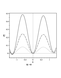
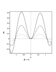
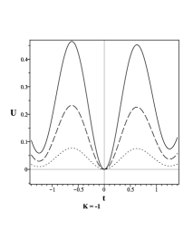
Figure 1: Graphs of vector fields in term of time. The solid, dash and doted lines represent $\xi=1$ ,$\frac{1}{6}$ and $0.5$ respectively.

As above mention we suggest following solution for $U_{i}(t)$

$$U_{i}(t)=\sqrt{A}e^{-\gamma t}\cos(mt+\theta),$$ (2.16)

where the parameter $A$ describes the oscillating amplitude of the field with dimension of $[mass]^{2}$. Also $A$ is relation with the parameter $\xi$, this solution implies the damping magnitude of the oscillating vector field.

3 Bouncing behavior

We will start with a detailed examination on the necessary conditions required for a successful bounce. During the contracting phase, the scale factor $a(t)$ is decreasing, i.e., $\dot{a}<0$, and in the expanding phase we have $\dot{a}>0$. At the bouncing point $\dot{a}=0$ and around this point $\ddot{a}>0$ for a period of time. Equivalently in the bouncing cosmology the Hubble parameter $H$ runs across zero from $H<0$ to $H>0$ and $H=0$ at the bouncing point. A successful bounce requires around this point

$$\dot{H}=-4\pi G(\rho+p)+\frac{k}{a^{2}}>0.$$ (3.1)

At the point where the bounce occurs, Eqs. (2.8) and (2.9) reduce to

$$\rho_{b}=\frac{3}{2a^{2}}(\dot{U_{i}}^{2}+m^{2}U^{2}_{i})-\frac{9k}{a^{4}}\xi U_{i}^{2},$$ (3.2)

$$p_{b}=\frac{3}{2a^{2}}(\dot{U_{i}}^{2}-m^{2}U^{2}_{i})+\frac{3k}{a^{4}}\xi U_{i}^{2},$$ (3.3)

On the other hand, a successful bounce from Eqs. (2.6), (2.7) and (3.1) obtain in the form,

$$\dot{U_{i}}^{2}<\frac{1}{2}m^{2}U^{2}_{i}+\frac{k}{a^{2}}\xi U_{i}^{2}.$$ (3.4)

This result is similar to slow roll inflation. This means that one requires a flat potential where give rise to a point bounce for the model of vector field. From conditions (3.1), (3.4) it is clear that if we have bouncing solutions in open universe, then we have such behaviour for flat and closed universe as well. Now we solve above equation numerically by different value of $\xi$ on the curved universe that is plotted in Fig. 2.

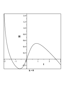
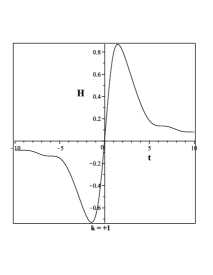
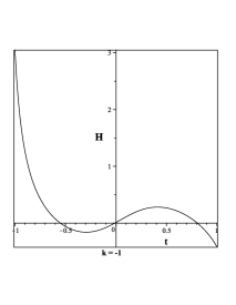
Figure 2: The graphs of the Hubble’s parameter for $\xi=1/6$, $4\pi G=1$, $m=1$ and $k=0,+1,-1$ by choosing $\phi(0)=1$, $\dot{\phi}(0)=0.1$, $a(0)=1$ and $H(0)=0.01$.

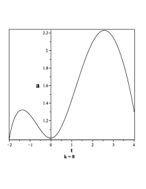
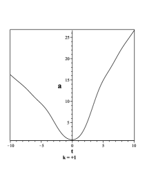
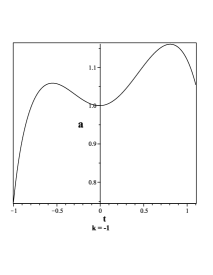
Figure 3: The graphs of the scale factor for $\xi=1/6$, $4\pi G=1$, $m=1$ and $k=0,+1,-1$ by choosing $\phi(0)=1$, $\dot{\phi}(0)=0.1$, $a(0)=1$ and $H(0)=0.01$.

One can see the Hubble parameter $H$ running across zero in any three cases of $k$. In all cases of $k$, we have $H<0$ to $H>0$ where implies to go from collapse era to an expanding era, and this result will not change for the different values $\xi$ in all of $k$. Also in Fig.3, we can see the behaviour of scale factor in terms of time for different values of $k$. It is clear that during the contracting phase, the scale factor $a(t)$ is decreasing, i.e., $\ddot{a}<0$, and in the expanding phase we have $\ddot{a}>0$, so the point where $\ddot{a}=0$ is bouncing point.
Therefore, in the vector field dominated universe we have a successful bouncing point in close and flat universe but a turn-around point in open universe. The bounce can be attributed to the negative-energy matter, which dominates at small values of $a$ and create a significant enough repulsive force so that a big crunch is avoided.

4 Reconstruction

Now we are going to present a reconstruction process for vector field in the curved universe by $\xi=1/6$ . In this section, potential and kinetic energy are reconstructed with respect to redshirt $z$. Also we obtain the EoS in term of $z$. After that three type parametrization are represented for the EoS. By using it we consider cosmology solutions such as the Eos, the deceleration parameter and vector field. The stability condition of this system is described by quantity of the sound speed. We rewrite Eqs. (2.14) and (2.15) in term of the effective potential energy $\hat{V}$ and the effective kinetic energy $\hat{K}$ as the following form,

$$\rho=\frac{3}{2}\dot{\phi_{i}}^{2}+\frac{3}{2}m^{2}\phi^{2}_{i}-\frac{3k}{2a^{2}}\phi^{2}_{i}=3\hat{K}+3\hat{V},$$ (4.1)

$$p=\frac{3}{2}\dot{\phi_{i}}^{2}-\frac{3}{2}m^{2}\phi^{2}_{i}+\frac{k}{2a^{2}}\phi^{2}_{i}=3\hat{K}-3\hat{V}-\frac{k}{a^{2}},$$ (4.2)

$$\rho+p=6\hat{K}-\frac{k}{a^{2}}.$$ (4.3)

Then we can write the Friedmann equations as following

$$3M^{2}_{p}(H^{2}+\frac{k}{a^{2}})=\rho_{m}+\rho=\rho_{m}+3\hat{K}+3\hat{V},$$ (4.4)

$$2M^{2}_{p}(\dot{H}-\frac{k}{a^{2}})=-\rho_{m}-\rho-p=-\rho_{m}-6\hat{K}+\frac{k}{a^{2}},$$ (4.5)

where $\rho_{m}$ is the energy density of dust matter. Also from Eqs. (4.1) and (4.2), we obtain relationship between the Eos with $\hat{V}$ and $\hat{K}$ as,

$$\omega=\frac{p}{\rho}=\frac{3\hat{K}-3\hat{V}-\frac{k}{a^{2}}}{3\hat{K}+3\hat{V}}=-1+\frac{2-\frac{k}{3a^{2}\hat{K}}}{1+\frac{\hat{V}}{\hat{K}}}.$$ (4.6)

We obviously have

$$\hat{V}+3\hat{K}>\frac{k}{3a^{2}}\Longrightarrow\omega>-1,$$

$$\hat{V}+3\hat{K}<\frac{k}{3a^{2}}\Longrightarrow\omega<-1,$$

$$\hat{V}+\hat{K}=\frac{k}{3a^{2}}\Longrightarrow\omega=-1.$$ (4.7)

By using Eqs. (4.4) and (4.5) we can write

$$\hat{K}=\frac{-\rho_{m}}{6}-\frac{M^{2}_{p}}{3}(\dot{H}-\frac{k}{3a^{2}})+\frac{k}{6a^{2}},$$ (4.8)

$$\hat{V}=\frac{M^{2}_{p}}{3}(3H^{2}+\dot{H}+\frac{2k}{a^{2}})-\frac{\rho_{m}}{6}-\frac{k}{6a^{2}}.$$ (4.9)

As in the present model, the dark energy fluid does not couple to the background fluid, the expression of the energy density of dust matter in respect of redshift $z$ is [18],

$$\rho_{m}=3M^{2}_{p}H^{2}_{0}\Omega_{m_{0}}(1+z)^{3},$$ (4.10)

where $\Omega_{m_{0}}$ is the ratio density parameter of matter fluid and the subscript $0$ indicates the present value of the corresponding quantity. By using the equation $1+z=\frac{a_{0}}{a}$ ($a_{0}$ is quantity given at the present epoch) and its differential form in following have,

$$\frac{d}{dt}=-H(1+z)\frac{d}{dz}.$$ (4.11)

To introduce a new variable $r$ as,

$$r=\frac{H^{2}}{H^{2}_{0}},$$ (4.12)

we rewrite the equation of motion of vector field against $z$ as,

$$2r(1+z)^{2}U^{\prime\prime}_{i}+2r(1+z)(1+H^{2}_{0})U^{\prime}_{i}-r^{\prime}(1+z)^{2}U^{\prime}_{i}$$

$$+r^{\prime}(1+z)U_{i}-rU_{i}+\frac{2m^{2}}{H^{2}_{0}}U_{i}-\frac{2k}{a^{2}_{0}H^{2}_{0}}(1+z)^{2}U_{i}=0,$$ (4.13)

$\hat{K}$, $\hat{V}$ can be rewrite as following

$$\hat{K}=-\frac{1}{2}M^{2}_{p}H^{2}_{0}\Omega_{m0}(1+z)^{3}+\frac{1}{6}M^{2}_{p}H^{2}_{0}r^{\prime}(1+z)+\frac{k}{6a_{0}^{2}}(1+z)^{2},$$ (4.14)

$$\hat{V}=M^{2}_{p}H^{2}_{0}r+\frac{2k}{3a_{0}^{2}}(1+z)^{2}-\frac{1}{6}M^{2}_{p}H^{2}_{0}(1+z)r^{\prime}-\frac{1}{2}M^{2}_{p}H^{2}_{0}\Omega_{m0}(1+z)^{3}-\frac{k}{6a_{0}^{2}}(1+z)^{2}.$$ (4.15)

By using Eqs. (4.6), (4.8) and (4.9) we obtain following expression for the EoS,

$$\omega=\frac{(1+z)r^{\prime}-3r+\frac{k(1+z)^{2}}{a_{0}^{2}H^{2}_{0}M^{2}_{p}}(M^{2}_{p}-2)}{3r-3\Omega_{m0}(1+z)^{3}+\frac{k(1+z)^{2}}{a_{0}^{2}H^{2}_{0}M^{2}_{p}}(M^{2}_{p}+2)}.$$ (4.16)

Then we obtain following equation for $r(z)$

$$r(z)=\Omega_{m0}(1+z)^{3}+(1-\Omega_{m0})e^{\beta(z)}$$

$$+\alpha_{0}\int^{z}_{0}\left[\omega(\tilde{z})(2+M^{2}_{p})+(2-M^{2}_{p})\right](1+\tilde{z})e^{-\beta(\tilde{z})}d\tilde{z}.$$ (4.17)

where $\beta(z)=\int^{z}_{0}\frac{3w(\tilde{z})}{1+\tilde{z}}d\tilde{z}$ and $\alpha_{0}=\frac{k}{a_{0}^{2}H^{2}_{0}M^{2}_{p}}$.

$$r(z)=\Omega_{m0}(1+z)^{3}+(1-\Omega_{m0})e^{3\int^{z}_{0}}\frac{1+w(\tilde{z})}{1+\tilde{z}}d\tilde{z}.$$ (4.18)

Also we have following expression for deceleration parameter q

$$q(z)=-1-\frac{\dot{H}}{H^{2}}=\frac{(1+z)r^{\prime}-2r}{2r}.$$ (4.19)

Now we consider the stability of this model by use the hydrodynamic analogy and judge on stability by examining the value of the sound speed. Of course this is a simple approach, the perturbations in vector inflation are much richer than in hydrodynamic model, see recent interesting works in [19, 20]. The sound speed can be obtained by the following equation,

$$c^{2}_{s}=\frac{p^{\prime}}{\rho^{\prime}}=\frac{-2r^{\prime}+(1+z)r^{\prime\prime}+2\frac{k(1+z)}{a_{0}^{2}H^{2}_{0}M^{2}_{p}}(M^{2}_{p}-2)}{-9\Omega_{m0}(1+z)^{2}+3r^{\prime}+2\frac{k(1+z)}{a_{0}^{2}H^{2}_{0}M^{2}_{p}}(M^{2}_{p}+2)},$$ (4.20)

in order to deal the stability of our model, the sound speed must become $c^{2}_{s}\geq 0$, so we can obtain from above equation following condition

$$r(z)\geq\omega_{m0}(1+z)^{3}-\frac{16ka^{2}_{0}}{H^{2}_{0}(1+z)^{2}}.$$ (4.21)

5 Parametrization

Now we consider the three different forms of parametrization as following and compare them together.
Parametrization 1: First Parametrization has proposed by Chevallier and Polarski [21],and Linder [22], where the EoS of dark energy in term of redshift $z$ is given by,

$$\omega(z)=\omega_{0}+\frac{\omega_{a}z}{1+z}.$$ (5.1)

Parametrization 2: Another the EoS in term of redshift z has proposed by Jassal, Bagla and Padmanabhan [23] as,

$$\omega(z)=\omega_{0}+\frac{\omega_{b}z}{(1+z)^{2}}.$$ (5.2)

Parametrization 3: Third parametrization has proposed by Alam, Sahni and Starobinsky [24]. They take expression of r in term of $z$ as followoing,

$$r(z)=\Omega_{m0}(1+z)^{3}+A_{0}+A_{1}(1+z)+A_{2}(1+z)^{2}.$$ (5.3)

By using the results of Refs. [25], [26], [27] and [28], we get coefficients of parametrization $1$ as $\Omega_{m0}=0.29$, $\omega_{0}=-1.07$ and $\omega_{a}=0.85$, coefficients of parametrization $2$ as $\Omega_{m0}=0.28$, $\omega_{0}=-1.37$ and $\omega_{b}=3.39$ and coefficients of parametrization $3$ as $\Omega_{m0}=0.30$, $A_{0}=1$, $A1=-0.48$ and $A2=0.25$. The evolution of $\omega(z)$ and $q(z)$ are plotted in Fig. 3. Also, using Eqs. (4.14) and (4.15) and the three parametrization, the evolutions of $\hat{K(z)}$ and $\hat{V(z)}$ are shown in Fig. 5 and Fig. 6 respectively. We note that graphs simply represent only in the flat universe.

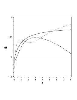
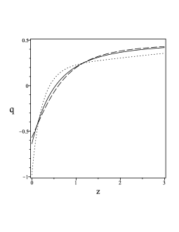
Figure 4: Graphs of the EoS and deceleration parameter in respect of redshift $z$. The solid, dot and dash lines represent parametrization 1, 2 and 3, respectively.

Figure 5: Graphs of the reconstructed $\hat{K}$ in respect of redshift $z$. The solid, dot and dash lines represent parametrization 1, 2 and 3, respectively.

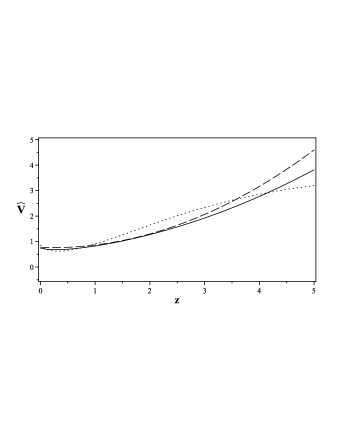
Figure 6: Graphs of the reconstructed $\hat{V}$ in respect of redshift $z$. The solid, dot and dash lines represent parametrization 1, 2 and 3, respectively.

From Figs. 4, 5 and 6, we can see parametrization $1$ and $3$ are same nearly and have slightly different from parametrization $2$. The EoS for any parametrization show in Fig. (4) so that they running cross to $-1$. Acceleration for all of parametrization shows to tend to the positive value. The $\hat{K}$ and $\hat{V}$ increase for parametrization $1$ and $3$, but in parametrization $2$ increase (decrease) for the $\hat{V}$ ($\hat{K}$). One can see that parametrization 1 and 3 satisfy condition $\hat{K}+\hat{V}>0$ and parametrization 2 satisfy condition $\hat{K}+\hat{V}=Constant$. In order to by Eq. (4), we have $\omega>-1$ ($\omega=-1$) when parametrization 1 and 3 (parametrization 2). This is mean that parametrization 2 is better than others parametrization.

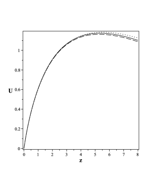
Figure 7: Graphs of the reconstructed $U_{i}$ in respect of redshift $z$. The solid, dot and dash lines represent parametrization 1, 2 and 3, respectively.

In Fig. 6, we can see the variation of the vector field against redshift $z$. One is obviously showed slightly difference between all of parametrization.

6 Conclusion

In this paper, we have studied the bouncing solution in curved universe which proposed by the model of a massive vector field, $U_{i}$, non-minimally coupled to gravity. For our purpose we have derived the corresponding energy density, pressure and Friedmann equation for this model. Also we have obtained the bouncing condition as Eq.(3.4). From this condition, and also essential condition (3.1), it is clear that if we have bouncing solutions in open universe, then we have such behaviour for flat and closed universe as well. After we plot the Hubble parameter in term of time by figures 2, for different $k$, we understood that our model predict the bouncing behavior for all cases of $k$. Fro these figures one can see that the Hubble parameter $H$ running across zero in any three cases of $k$. In all cases of $k$, we have $H<0$ to $H>0$ where implies to go from collapse era to an expanding era, and this result will not change for the different values $\xi$ in all of $k$. After that in figures 3 we have shown that during the contracting phase, the scale factor $a(t)$ is decreasing, i.e., $\ddot{a}<0$, and in the expanding phase we have $\ddot{a}>0$, so the point where $\ddot{a}=0$ is bouncing point, and this figure is consistent with the results of Fig 2.
After that we have investigated an interesting method as the reconstruction of the non-minimally coupled massive vector field model with the action (2.1). Our aim was to see whether the non-minimal coupling vector field can actually reproduce required values of observable cosmology, such as evolution of the EoS and the deceleration parameter in respect to the redshift $z$. We have reconstructed our model in three different forms of parametrization for massive vector field. In Fig. 4 we have found the EoS crossing $-1$ in all of parametrization. The variation of reconstructed kinetic and potential energy against $z$ have plotted in Figs. 5 and 6, where the parametrization 2 in addition is better than two others parametrization because $\hat{K}+\hat{V}=Constant$. Also we have investigated the stability of this system and have obtained a condition by the sound speed in all of curvatures. Finally we note that reconstructed physical quantities have just executed in flat universe and one is suggested for open and close universe as future work.

7 Acknowledgment

The authors are indebted to the anonymous referee for his/her comments that improved the paper drastically.

References

- [1] A. Golovnev, V. Mukhanov and V. Vanchurin, JCAP 0806, 009 (2008).
- [2] T. Chiba,arXiv:0805.4660v3 [gr-qc]2008
- [3] A. G. Riess et al. [Supernova Search Team Collaboration], Astron. J. 116, 1009 (1998) [astro-ph/9805201]; S. Perlmutter et al. [Supernova Cosmology Project Collaboration], Astrophys. J. 517, 565 (1999) [astro-ph/9812133]; P. Astier et al., Astron. Astrophys. 447, 31 (2006) [astro-ph/0510447].
- [4] K. Abazajian et al. [SDSS Collaboration], Astron. J. 128, 502 (2004) [astro-ph/0403325]; K. Abazajian et al. [SDSS Collaboration], Astron. J. 129, 1755 (2005) [astro-ph/0410239].
- [5] D. N. Spergel et al. [WMAP Collaboration], Astrophys. J. Suppl. 148, 175 (2003) [astro-ph/0302209]; D. N. Spergel et al., astro-ph/0603449.
- [6] A. H. Guth, Phys. Rev. D 23, 347, (1981).
- [7] Peebles, P.J.E., Ratra, B.: Astrophys. J. 325, L17 (1988); Ratra, B., Peebles, P.J.E.: Phys. Rev. D 37, 3406 (1988); Wetterich, C.: Nucl. Phys. B 302, 668 (1988); Caldwell, R.R., Dave, R., Steinhardt, P.J.: Phys. Rev. Lett. 80, 1582 (1998). astro-ph/9708069; Liddle, A.R., Scherrer, R.J.: Phys. Rev. D 59, 023509 (1999). astro-ph/9809272; Zlatev, I., Wang, L.M., Steinhardt, P.J.: Phys. Rev. Lett. 82, 896 (1999). astro-ph/9807002; Faraoni, V. Phys. Rev. D62, 023504 (2000); Huang, Z.G., Lu, H.Q., Fang, W.: Class. Quantum Gravity 23, 6215 (2006). hep-th/0604160
- [8] Armendariz-Picon, C., Mukhanov, V.F., Steinhardt, P.J.: Phys. Rev. Lett. 85, 4438 (2000). astro-ph/ 0004134; Armendariz-Picon, C., Mukhanov, V.F., Steinhardt, P.J.: Phys. Rev. D 63, 103510 (2001). astro-ph/ 0006373; Chiba, T., Okabe, T., Yamaguchi, M.: Phys. Rev. D 62, 023511 (2000)
- [9] Sen, A.: J. High Energy Phys. 0207, 065 (2002); Padmanabhan, T. Phys. Rev. D 66, 021301 (2002).; Setare, M. R. Phys. Lett. B 653, 116 (2007); M. R. Setare, J. Sadeghi, A. R. Amani, Phys. Lett. B 673, 241, (2009).
- [10] Caldwell, R. R. Phys. Lett. B 545, 23 (2002). astro-ph/9908168; Caldwell, R. R., Kamionkowski, M., Weinberg, N. N. Phys. Rev. Lett. 91, 071301 (2003). astro-ph/ 0302506; Nojiri, S., Odintsov, S.D.: Phys. Lett. B 562, 147 (2003). hep-th/0303117; Nojiri, S., Odintsov, S. D. Phys. Lett. B 565, 1 (2003). hep-th/0304131; Faraoni, V. Class. Quantum Gravity 22, 3235 (2005); Setare, M. R. Eur. Phys. J. C 50, 991 (2007)
- [11] Piazza, F., Tsujikawa, S., J. Cosmol. Astropart. Phys. 0407, 004 (2004). hep-th/0405054
- [12] L. H. Ford, Phys. Rev. D 40, 967 (1989).
- [13] Armendariz-Picon C, JCAP 07(2004)007.
- [14] A. Borde, A. Guth, A. Vilenkin, Phys. Rev. Lett. 90, 151301 (2003), gr-qc/0110012.
- [15] M. Novello and J. Salim, Phys. Rev. D 20, 377 (1979).
- [16] V. N. Melnikov and S. V. Orlov, Phys. Lett. A 70, 263 (1979).
- [17] M. Novello, S. E. Perez Bergliaffa, arXiv:0802.1634 [astro-ph].
- [18] S. Zhang, B. Chen, Phys. Lett. B 669, 4 (2008); M. R. Setare, J. Sadeghi, A. Banijamali, Phys. Lett. B 669, 9, (2008); M. R. Setare , J. Sadeghi and A. R. Amani ,Int. J. Mod. Phys. D 18, 1291, (2009).
- [19] B. Himmetoglu, C. R. Contaldi, M. Peloso, Phys. Rev. D 79, 063517, (2009); B. Himmetoglu, C. R. Contaldi, M. Peloso, arXiv:0909.3524v1 [astro-ph.CO]; B. Himmetoglu, C. R. Contaldi, M. Peloso, Phys. Rev. Lett. 102, 111301, (2009).
- [20] A. Golovnev, arXiv:0910.0173v4 [astro-ph.CO]; A. Golovnev, V. Vanchurin, Phys. Rev. D 79, 103524, (2009).
- [21] M. Chevallier and D. Polarski, Int. J. Mod. Phys. D 10, 213 (2001).
- [22] E. V. Linder, Phys. Rev. Lett. 90, 091301 (2003).
- [23] H. K. Jassal, J. S. Bagla and T. Padmanabhan, Mon. Not. Roy. Astron. Soc. 356, L11 (2005). 11
- [24] U. Alam, V. Sahni, T. D. Saini and A. A. Starobinsky, Mon. Not. Roy. Astron. Soc. 354, 275 (2004).
- [25] A. G. Riess et al. [Supernova Search Team Collaboration], [arXiv:astro-ph/0611572].
- [26] Y. G. Gong and A. Z. Wang, Phys. Rev. D 75, 043520, (2007).
- [27] Y. Wang and P. Mukherjee, Astrophys. J. 650, 1 (2006).
- [28] D. J. Eisenstein et al. [SDSS Collaboration], Astrophys. J. 633, 560 (2005).