Rapidity correlations of protons from a fragmented fireball

Abstract

We investigate proton rapidity correlations for a fireball that fragments due to non-equilibrium effects at the phase transition from deconfined to hadronic phase. Such effects include spinodal fragmentation in case of first order phase transition at lower collision energies, and cavitation due to sudden rise of the bulk viscosity at the crossover probed at RHIC and the LHC. Our study is performed on samples of Monte Carlo events. Correlation function in relative rapidity appears to be a sensitive probe of fragmentation. We show that resonance decays make the strength of the correlation even stronger.

1 Introduction

Exploration of properties of very hot strongly interacting matter is the main goal for which experiments with colliding heavy atomic nuclei at ultrarelativistic energies are performed. The suggested phase diagram shows rapid but smooth crossover from confined to deconfined matter at temperatures around 170 MeV and vanishing baryochemical potential Aoki:2006we . The smooth crossover becomes a first order phase transition at some, presently not precisely known, value of the baryochemical potential Stephanov:2004wx ; Fodor:2004nz . To find the layout of the phase diagram is one of the main goals of present theoretical as well as experimental activity in the field.

The fireball which is created in nuclear collisions expands rapidly and so the evolution can proceed out of the equilibrium. Particularly, passage of the bulk through the phase transition or the crossover can be too fast and non-equilibrium scenario could be relevant. In case of the first order phase transition this would lead to supercooling Csernai:1995zn . Even maximum possible supercooling and subsequent spinodal decomposition could happen Mishustin:1998eq ; Mishustin:2001re ; Scavenius:2000bb . There, the bulk becomes mechanically unstable and fragments into droplets of high temperature phase. At RHIC and the LHC we likely have the smooth crossover, however. Nevertheless, in this case calculations show a sharp rise of the bulk viscosity prattbulk ; kharbulk ; Meyer:2007dy which might lead to fireball fragmentation Torrieri:2007fb ; Torrieri:2008ip ; Rajagopal:2009yw , as well. Thus the passage through the phase transition can in any case lead to fragmentation of the fireball into smaller droplets which then evaporate hadrons.

Then, the relevant question is: How does one recognise the fragmentation of the bulk? Correlations of hadrons are a good candidate for an observable which would be sensitive to fragmentation. Hadrons originating from the same fragment will have correlated velocities. Their velocities would be centered around the velocity of the fragment. It has been proposed long time ago pratt94 and reexamined more recently randrup05 that proton correlations are appropriate observables to look at. Protons are rather abundant in nuclear collisions and their velocities are close to the velocities of the fragments. This is due to the large proton mass which leads to small thermal velocities of protons. Pions, in comparison, are much more abundant but also very light. Hence, their velocities may differ considerably from the velocities of the emitting fragments and their correlation function is less suitable to study the effect of fragmentation.

In this paper we study proton correlations in rapidity on datasets simulated with a realistic Monte Carlo event generator DRAGON dragon . This is an improvement over previous simulations randrup05 where only a schematic distribution of droplets has been used. In our model, droplets have sizes distributed according to gamma-distribution and their positions are random with the only constraint that they must not overlap. It is also important that resonance decays are included. We investigate the effect of resonances on proton correlations.

In the following section we define the correlation functions which have been measured. In Section 3 we give a short overview about DRAGON. Results are presented in Section 4 where we also discuss our predictions for FAIR and the LHC. Conclusions are given in Section 5.

2 The correlation function

We shall measure the correlation function in kinematic variable $\Delta x$ (e.g. rapidity difference)

$$C(\Delta x)=\frac{\Phi_{2}(\Delta x)}{\Phi_{2,\mathrm{mixed}}(\Delta x)}$$ (1)

where $\Phi_{2}(\Delta x)$ is the probability to observe a pair of hadrons with the distance $\Delta x$. It is averaged over all events of the sample. Denominator $\Phi_{2,\mathrm{mixed}}(\Delta x)$ is the reference distribution obtained by the mixed events technique. Hence, $\Phi_{2,\mathrm{mixed}}(\Delta x)$ is only determined by the overall distribution of hadrons and not affected by any correlations.

In our study, as $\Delta x$ we shall use the rapidity difference

$$\Delta y=y_{1}-y_{2}\,,$$ (2)

and the relative rapidity

$$y_{12}=\ln\left[\gamma_{12}+\sqrt{\gamma_{12}^{2}-1}\right]$$ (3)

with

$$\gamma_{12}=\frac{p_{1}\cdot p_{2}}{m_{1}m_{2}}\,.$$ (4)

Note that $y_{12}$ is the rapidity that corresponds to relative velocity of one particle in the rest frame of the other

$$y_{12}=\frac{1}{2}\ln\left(\frac{1+v_{12}}{1-v_{12}}\right)\,.$$ (5)

In the following we re-derive the correlation function randrup05 in $\Delta y$ for the simple case where protons are emitted from droplets distributed according to Gaussian distribution. The two proton distribution in rapidity in one event is written as a sum of two terms, one corresponding to both protons coming from the same droplet, other to each proton stemming from a different droplet

$$\rho_{2}(y_{1},y_{2})=\sum_{i}\rho_{2}^{i}(y_{1},y_{2})+\sum_{i\neq j}\rho_{1}^{i}(y_{1})\rho_{1}^{j}(y_{2})\,.$$ (6)

Here, $i,j$ numerate the droplets and $\rho_{1}^{i}$ are the single-particle distributions for production from one droplet

$$\rho_{1}^{i}(y)=\frac{\nu_{i}}{\sqrt{2\pi\sigma^{2}}}\exp\left(-\frac{(y-y_{i})^{2}}{2\sigma^{2}}\right)\,.$$ (7)

The droplet is thus centred around $y_{i}$ and its rapidity distribution has the width $\sigma_{i}$; $\rho_{1}^{i}(y)$ is normalized to the total number of protons from this droplet $\nu_{i}$

$$\int\rho_{i}^{i}(y)\,dy=\nu_{i}\,.$$ (8)

The two-proton distribution for one droplet is then

$$\rho_{2}^{i}(y_{1},y_{2})=\\ \frac{\nu_{i}(\nu_{i}-1)}{{2\pi\sigma^{2}}}\,\exp\left(-\frac{(y_{1}-y_{i})^{2}}{2\sigma^{2}}\right)\,\exp\left(-\frac{(y_{2}-y_{i})^{2}}{2\sigma^{2}}\right)$$ (9)

and is normalized to the total number of proton pairs from the droplet

$$\int\rho_{2}^{i}(y_{1},y_{2})\,dy_{1}\,dy_{2}=\nu_{i}(\nu_{i}-1)\,.$$ (10)

The sums in (6) run over all droplets and over all pairs of droplets in the event.

We next introduce two-particle distribution in rapidity difference in one event

$$F(\Delta y) = \int dy_{1}\,dy_{2}\,\delta(\Delta y-(y_{1}-y_{2}))\,\rho_{2}(y_{1},y_{2})$$ (11)

$$= \int dy_{1}\,dy_{2}\,\delta(\Delta y-(y_{1}-y_{2}))$$

$$\times\left[\sum_{i}\rho_{2}^{i}(y_{1},y_{2})+\sum_{i\neq j}\rho_{2}^{i}(y_{1})\rho_{2}^{j}(y_{2})\right]\,.$$

This leads to

$$F(\Delta y)=\frac{1}{2}\frac{1}{\sqrt{\pi\sigma^{2}}}\Biggl{[}\exp\left(-\frac{\Delta y^{2}}{4\sigma^{2}}\right)\sum_{i}\nu_{i}(\nu_{i}-1)\\ +\sum_{i\neq j}\nu_{i}\nu_{j}\exp\left(-\frac{\Delta y-(y_{i}-y_{j})}{4\sigma^{2}}\right)\Biggr{]}\,.$$ (12)

In order to obtain $\Phi_{2}(\Delta y)$, this must be now averaged over a large sample of events. By doing this we shall also sum over many droplets. In the first term on the r.h.s. of eq. (12) this leads to

$$\frac{1}{N_{\mathrm{ev}}}\sum_{\mathrm{events}\,\alpha}\sum_{i}\nu_{i,\alpha}(\nu_{i,\alpha}-1)=\langle N_{d}\rangle\langle\nu(\nu-1)\rangle_{M}$$ (13)

where the subscript $i$ numbers droplets in one event and $\alpha$ stands for different events; $\langle N_{d}\rangle$ is the average number of droplets per event and $\langle\dots\rangle_{M}$ denotes averaging over multiplicity distribution for one droplet. Thus $\langle\nu(\nu-1)\rangle_{M}$ stands for the average number of proton pairs from one droplet. Assuming further that droplet centres are distributed according to Gaussian distribution with the width $\xi$

$$\zeta(y_{d})=\frac{1}{\sqrt{2\pi\xi^{2}}}\,\exp\left(-\frac{(y_{d}-y_{0})^{2}}{2\xi^{2}}\right)$$ (14)

we can derive that

$$\Phi_{2}(\Delta y)=\frac{1}{2}\,\frac{1}{\sqrt{\pi\sigma^{2}}}\,\langle N_{d}\rangle\langle\nu(\nu-1)\rangle_{M}e^{-\frac{\Delta y^{2}}{4\sigma^{2}}}\\ +\frac{1}{2}\,\frac{1}{\sqrt{\pi(\xi^{2}+\sigma^{2})}}\langle N_{d}(N_{d}-1)\rangle\langle\nu\rangle_{M}^{2}e^{-\frac{\Delta y^{2}}{4(\xi^{2}+\sigma^{2})}}\,.$$ (15)

The denominator of the correlation function is constructed from the mixed pairs sample. Hence, there are no pairs where both protons would be emitted from the same droplet. The single-particle rapidity distribution is determined by integrating over all possible droplet positions

$$\tau(y) = \int\frac{1}{\sqrt{2\pi\sigma}}\,\exp\left(-\frac{(y-\chi)^{2}}{2\sigma^{2}}\right)$$ (16)

$$\qquad\qquad\times\frac{1}{\sqrt{2\pi\xi^{2}}}\exp\left(-\frac{(\chi-y_{0})^{2}}{2\xi^{2}}\right)\,d\chi$$

$$= \frac{1}{\sqrt{2\pi(\xi^{2}+\sigma^{2})}}\,\exp\left(-\frac{(y-y_{0})^{2}}{2(\xi^{2}+\sigma^{2})}\right)\,.$$

Note that this distribution is normalized to unity. Thus to get $\Phi_{2,\mathrm{mixed}}(\Delta y)$ normalized to average number of pairs per event, we calculate

$$F_{\mathrm{mixed}}(\Delta y)=\langle N_{d}\rangle\langle\nu\rangle_{M}\left(\langle N_{d}\rangle\langle\nu\rangle_{M}-1\right)\\ \times\int dy_{1}dy_{2}\,\delta(\Delta y-(y_{1}-y_{2}))\,\tau(y_{1})\tau(y_{2})\,.$$ (17)

Mixed events are by construction averaged over a large number of events and thus we can write directly

$$\Phi_{2,\mathrm{mixed}}(\Delta y)=F_{\mathrm{mixed}}(\Delta y)\\ =\frac{1}{2}\frac{\langle N_{d}\rangle\langle\nu\rangle_{M}\left(\langle N_{d}\rangle\langle\nu\rangle_{M}-1\right)}{\sqrt{\pi(\xi^{2}+\sigma^{2})}}\,\exp\left(-\frac{\Delta y^{2}}{4(\xi^{2}+\sigma^{2})}\right)\,.$$ (18)

This is almost identical—up to the term involving multiplicity averages—with the second term of the expression for $\Phi_{2}(\Delta y)$ (15). In practical evaluation, however, we shall normalize the correlation function so that it converges to unity for large $\Delta y$. This is equivalent to replacing

$$\langle N_{d}\rangle\langle\nu\rangle_{M}\left(\langle N_{d}\rangle\langle\nu\rangle_{M}-1\right)\to\langle N_{d}(N_{d}-1)\rangle\langle\nu\rangle_{M}^{2}\,.$$

Then we obtain

$$C(\Delta y)-1=\frac{\xi\langle N_{d}\rangle\langle\nu(\nu-1)\rangle_{M}}{\langle N_{d}(N_{d}-1)\rangle\langle\nu\rangle_{M}^{2}}\,\sqrt{1+\frac{\sigma^{2}}{\xi^{2}}}\,\frac{1}{\sigma}\\ \times\exp\left(-\frac{\Delta y^{2}}{4\sigma^{2}\left(1+\frac{\sigma^{2}}{\xi^{2}}\right)}\right)\,.$$ (19)

Here we see that the correlation function will have the width given by $\sigma\sqrt{1+\sigma^{2}/\xi^{2}}$. Note that $\xi$ is the width of the droplet distribution in rapidity, thus the density of droplets will be proportional to

$$n_{d}\sim\frac{\langle N_{d}\rangle}{\xi}\,.$$ (20)

Based on this, for large $\langle N_{d}\rangle$

$$\frac{\xi\langle N_{d}\rangle}{\langle N_{d}(N_{d}-1)\rangle}\sim\frac{1}{n_{d}}$$ (21)

so the magnitude of the correlation function is inversely proportional to the rapidity density of the droplets. This is quite natural: In a dense configuration of many small droplets—resembling a fog—the system becomes homogeneous and correlation function should be trivial.

Note that the choice of Gaussian distribution in this argumentation is only due to technical simplicity. Qualitatively, the conclusions are more general.

3 The Monte Carlo event generator

Monte Carlo events are prepared with DRAGON: Droplet and hadron generator for nuclear collisions. Detailed description is available in dragon . Here we summarize the main features of the model and introduce parameters which are varied in subsequent studies.

Hadrons, including resonances, can be directly produced either from the bulk fireball or from the decaying droplets. The fraction of those hadrons emitted from droplets is a parameter that can be set. Resonances decay according to standard two and three-body kinematics with constant matrix element. Chain decays are possible. Expected $dN/dy$ or the total multiplicity, which is an experimental observable, is among the input parameters. This setting allows for relevant comparisons if the multiplicity is kept constant and hadron production is divided between bulk and droplet emission in different fractions.

Directly produced hadrons and the droplets are formed at the usual freeze-out hypersurface of the blast wave model. It is characterized by constant longitudinal proper time $\tau=\sqrt{t^{2}-z^{2}}$. In this study we only investigate the case of central collisions and assume circular transverse profile of the fireball with a radius $R$. The fireball also exhibits an expansion pattern which is longitudinally boost invariant and has tunable gradient in the transverse direction. The expansion velocity profile is given as

$$u^{\mu}(x) = u^{\mu}(\eta,r,\phi)$$ (22)

$$= (\cosh\eta\,\cosh\eta_{t}(r),\,\cos\phi\,\sinh\eta_{t}(r),$$

$$\qquad\sin\phi\,\sinh\eta_{t}(r),\,\sinh\eta\,\cosh\eta_{t}(r))$$

$$\eta_{t}(r) = \sqrt{2}\rho_{0}\frac{r}{R}\,.$$ (23)

where we use the polar coordinates $r$ and $\phi$ in the transverse plane and the space-time rapidity

$$\eta=\frac{1}{2}\ln\frac{t+z}{t-z}\,.$$

These coordinates are taken in the centre of mass system of the collision.

Droplets are randomly placed within the fireball. Their volumes follow the Gamma distribution

$${\cal P}_{2}(V)=\frac{V}{b^{2}}e^{-V/b}\,,$$ (24)

where the volume parameter $b$ determines the average volume

$$\overline{V}=\frac{b}{2}\,.$$

The masses of the droplets are proportional to their volumes while the energy density is taken with the value 0.7 GeV.fm^-3. Their velocities are given by $u^{\mu}(x)$ at the position where they are produced. Droplets decay exponentially in time with the mean lifetime being equal to the radius of the droplet.

Hadrons, regardless if they come from a droplet or from bulk, are emitted from a thermal source with kinetic temperature $T_{\mathrm{kin}}$. In case of production from bulk, the thermal distribution is boosted with the local expansion velocity at the point of hadron emission. In case of production from a droplet the thermal distribution is assumed in the rest frame of the droplet.

Chemical composition of the produced hadrons is determined by the assumption of chemical equilibrium with temperature $T_{\mathrm{ch}}$. Chemical potentials correspond to conserved quantum numbers with baryonic chemical potential $\mu_{B}$ being a free parameter and strangeness chemical potential being set by the requirement of total strangeness neutrality.

Resonances with masses up to 1.5 GeV/$c^{2}$ (mesons) and 2 GeV/$c^{2}$ (baryons) according to the particle data book are included.

4 Results

Correlation functions are evaluated from samples of artificial events. Numerators are built as histograms including pairs of protons from the same event according to their relative rapidity. We investigate rapidity difference in 1 dimension, eq.(2), and the relative rapidity in three dimensions, eq.(3). Denominator of the correlation function is constructed from pairs of randomly chosen protons from different events. The constructed correlation functions are normalized so that they approach unity for large rapidity differences. The obtained data are fitted by Gaussian form

$$C(x)-1=A\exp\left(-\frac{x^{2}}{2\sigma^{2}}\right)\,,$$ (25)

where $x$ is replaced by either $y_{12}$ or $\Delta y$ and $A$, $\sigma$ are fit parameters.

Most detailed studies are performed on samples of events generated with RHIC parameter settings. Chemical composition is characterized by $T_{\textrm{ch}}=170$ MeV and $\mu_{B}=46$ MeV. Total hadron rapidity density is $dN/dy=1000$. (Note that this includes also neutral hadrons.) Kinetic temperature, if not stated otherwise, is put to 150 MeV. There is transverse flow with $\rho_{0}=0.7$. Rapidity distribution is uniform, but only hadrons from the interval $[-1,1]$ are taken into the analysis. For each parameter settings a sample of 10,000 events is generated.

We first consider the case of only partial production of hadrons (protons) from the droplets. In Fig. 1

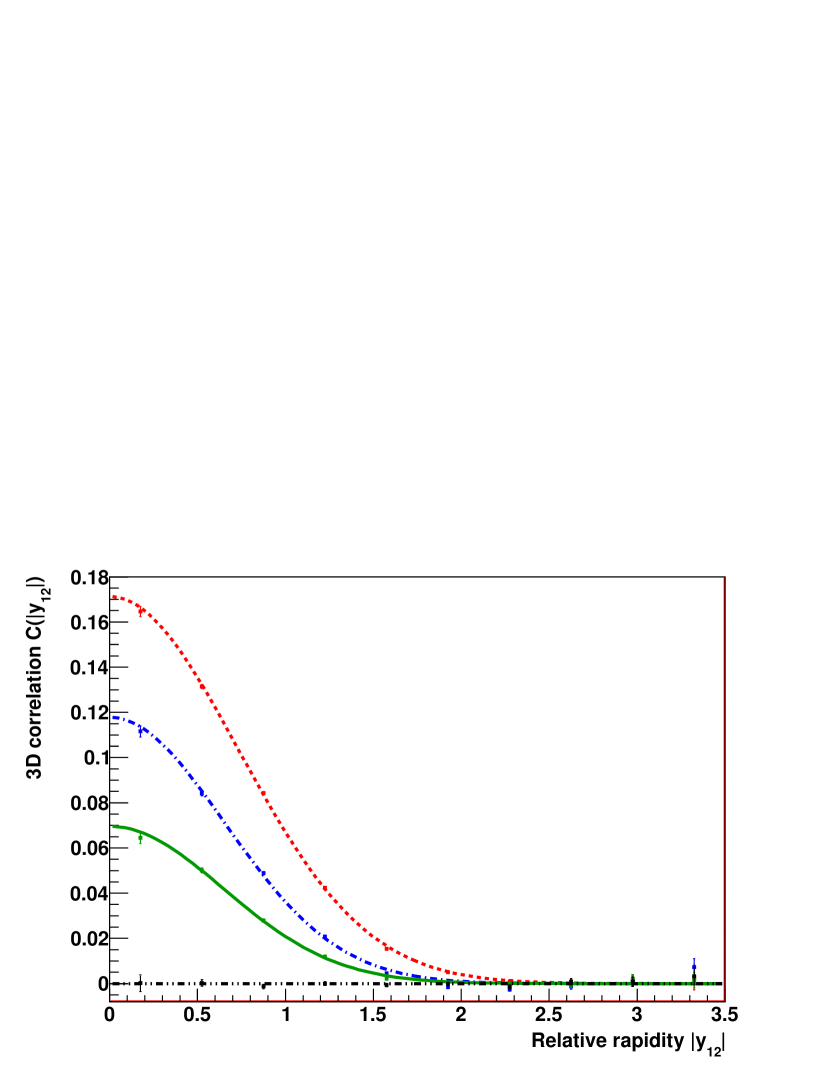
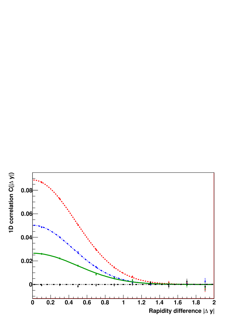
Figure 1: Correlation functions in $y_{12}$ (upper panel) and $\Delta y$ (lower panel) for RHIC parameter settings with $b=50\,\mathrm{fm}^{3}$ and varying fraction of droplet-emitted hadrons: $d=0$ (black dash-dot-dotted curves), $d=0.25$ (green solid), $d=0.5$ (blue dash-dotted), and $d=1$ (red dotted).

we keep the average size of droplets constant by fixing $b=50\,\mathrm{fm}^{3}$ and change the fraction of hadrons being emitted by the droplets. The other part comes from the bulk fireball while the multiplicity is kept constant. Clearly, at vanishing $d$ the correlation function is trivial. In both cases, for correlation functions in 1D variable $\Delta y$ and 3D variable $y_{12}$, the width is independent of the fraction $d$ while the correlation strength $A$ increases as more hadrons come from the droplets. We also see that the correlation is about a factor of 2 stronger if plotted as a function of $y_{12}$ (3D correlation). Therefore, in the following we shall only study correlation function in $y_{12}$.

The effect of varying the size of droplets is investigated in Fig. 2.

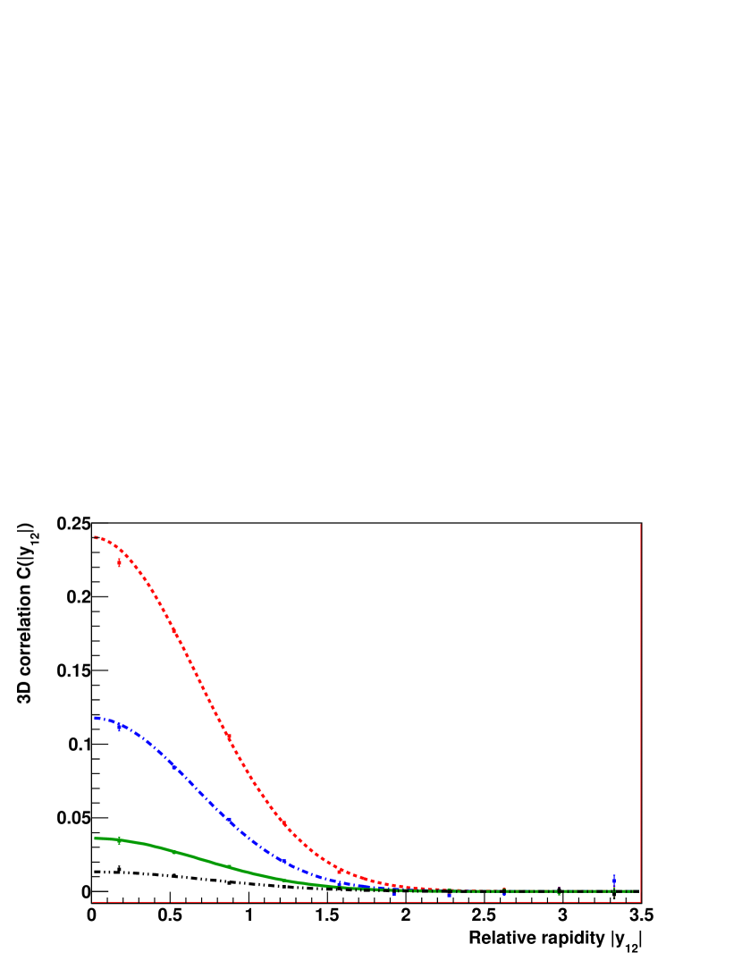
Figure 2: Correlation functions in $y_{12}$ for RHIC parameter settings with one half of hadrons coming from droplets, i.e. $d=0.5$. Different curves correspond to different sizes of the droplets: $b=10\,\mbox{fm}^{3}$ (black dash-dot-dotted curve), $b=20\,\mbox{fm}^{3}$ (green solid), $b=50\,\mbox{fm}^{3}$ (blue dash-dotted), and $b=100\,\mbox{fm}^{3}$ (red dotted).

Here, one half of all hadrons comes from droplets. Since large droplets correlate more protons, the strength of the correlation function is increased as $b$ grows. The correlation goes away when the droplets are so small that not enough energy is available for a proton pair creation. At $b=10\,\textrm{fm}^{3}$ the average mass of a droplet is 3.5 GeV which may be enough for two protons to be created, thus we still see correlation at the level of 0.01. At $b=5\,\textrm{fm}^{3}$ this decreases to 1.75 GeV which is insufficient for a proton pair and the correlation function would be trivial.

We observe that the correlation strength grows both with bigger droplets and/or with larger droplet fraction. The dependence of $A$ on $b$ and $d$ is studied in Fig. 3.

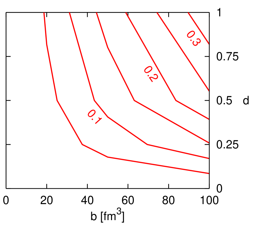
Figure 3: Contour plot shows the dependence of the amplitude $A$ of the correlation function calculated for RHIC as a function of droplet size parameter $b$ and fraction of particles from droplets $d$. The step between the contours is 0.05, labels show the corresponding value of the contours.

Here, we summarize the values which were obtained from fits to correlation functions. We conclude that it is not possible to determine the droplet size or the droplet fraction just from measuring the correlation strength $A$. The value of $A$ can at most help to establish a range of possible combinations of $b$ and $d$. If, however, one of them can be determined by some other means, then rapidity correlations can be used for the measurement of the other.

So far we have only investigated the variation of the correlation function with changing properties of the droplets. In Fig. 4

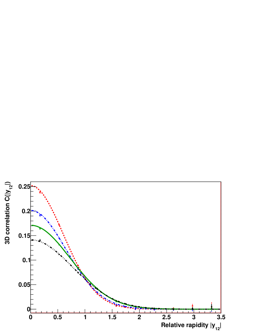
Figure 4: Correlation functions for RHIC parameters with all hadrons emitted from droplets and $b=50~{}\mbox{fm}^{3}$. Different curves correspond to different kinetic freeze-out temperatures: $T=170$ MeV (black dash-dot-dotted curve), $T=150$ MeV (green solid), $T=130$ MeV (blue dash-dotted), $T=110$ MeV (red dotted).

we study the effect of temperature variation. Average droplet volume is given by $b=50\,\mathrm{fm}^{3}$ and all hadrons are emitted from droplets. We observe weakening of the correlation as the temperature increases. The interpretation is at hand: the effect of the temperature is the smearing of hadron velocity so that it does not exactly follow that of the droplet. Therefore, lower temperature leads to increased correlations. Formally, this effect can be also seen in eq.(19) (although that equation was derived for $\Delta y$). Higher temperature translates into larger $\sigma$. Through the pre-factor $1/\sigma$ (at large $\xi$) this makes the correlation weaker.

Our model also allows for dedicated investigation of the effect of resonance decays on the observed correlations. This is shown in Fig. 5.

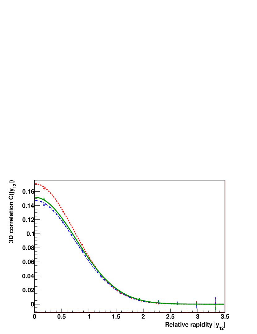
Figure 5: Correlation functions in $y_{12}$ for standard RHIC parameter settings with all particles emitted from droplets and $b=50\,\mbox{fm}^{3}$. Different curves show: full correlation function with all resonance decays included (red dotted curve), result from a simulation with no resonance production included (green solid), result from a simulation with resonances included but protons coming from decays of Delta resonances were not taken into analysis (blue dash-dotted).

We see that the resonances increase the intercept of the correlation function, i.e., they strengthen the correlation. This is a result of two effects: in resonance decay, daughter particles obtain some momentum due to the mass difference between the resonance and its decay products. This would lead to more smearing of the final hadron momenta and lower correlation. On the other hand, resonances are heavier and therefore closer to the velocity of the emitting droplet than lighter hadrons. This increases the correlation. Eventually, the second effect wins and the correlation function is increased. Note that the smearing of resonance momentum in production from the droplet gets weaker if the temperature is lowered. Since in our simulation we calculate with rather high kinetic freeze-out temperature of 150 MeV, it can be expected that this effect will always dominate the influence on the correlation function.

In Fig. 5 we also see that the dominant contribution within the resonance decays that produce protons comes from the deltas.

We next turn to predictions of the proton rapidity correlations at other collision energies. First is that of few GeV per nucleon. This is the domain that should be studied with the help of the planned programs at low energy RHIC run, SPS energy scan, FAIR in Darmstadt, and NICA at the JINR Dubna. This energy domain seems important since the critical point of the QCD phase diagram is suspected to be here. If so, these accelerators might bring us into the region of the phase diagram with first order phase transition where spinodal decomposition Mishustin:1998eq ; Mishustin:2001re and subsequent emission of hadrons from droplets can happen.

For FAIR energy we choose Gaussian profile of the fireball in the space-time rapidity $\eta$, with the width $\Delta\eta=0.7$. Chemical composition is taken from the analysis of Pb+Pb collisions at CERN SPS at projectile energy 40 $A$ GeV Becattini:2003wp : chemical freeze-out temperature is 140 MeV and the baryochemical potential is 428 MeV. Kinetic freeze-out temperature agrees with that of chemical freeze-out. Again, there is transverse flow with $\rho_{0}=0.4$. The total multiplicity is 1250. As a result, on average there are 135 protons per event. Results on the correlation functions are very similar to those obtained for RHIC energy and are therefore not shown separately.

We also make simulations for a fireball as expected in Pb+Pb collisions at the LHC. Due to near nuclear transparency the baryochemical potential is taken at 1 MeV while the chemical freeze-out temperature is 170 MeV. Kinetic freeze out temperature is set to 150 MeV and there is slightly higher transverse expansion gradient $\rho_{0}=0.8$. Multiplicity density $dN/dy=2000$.

Since results at all investigated collision energies are qualitatively very similar, we only show in Fig. 6

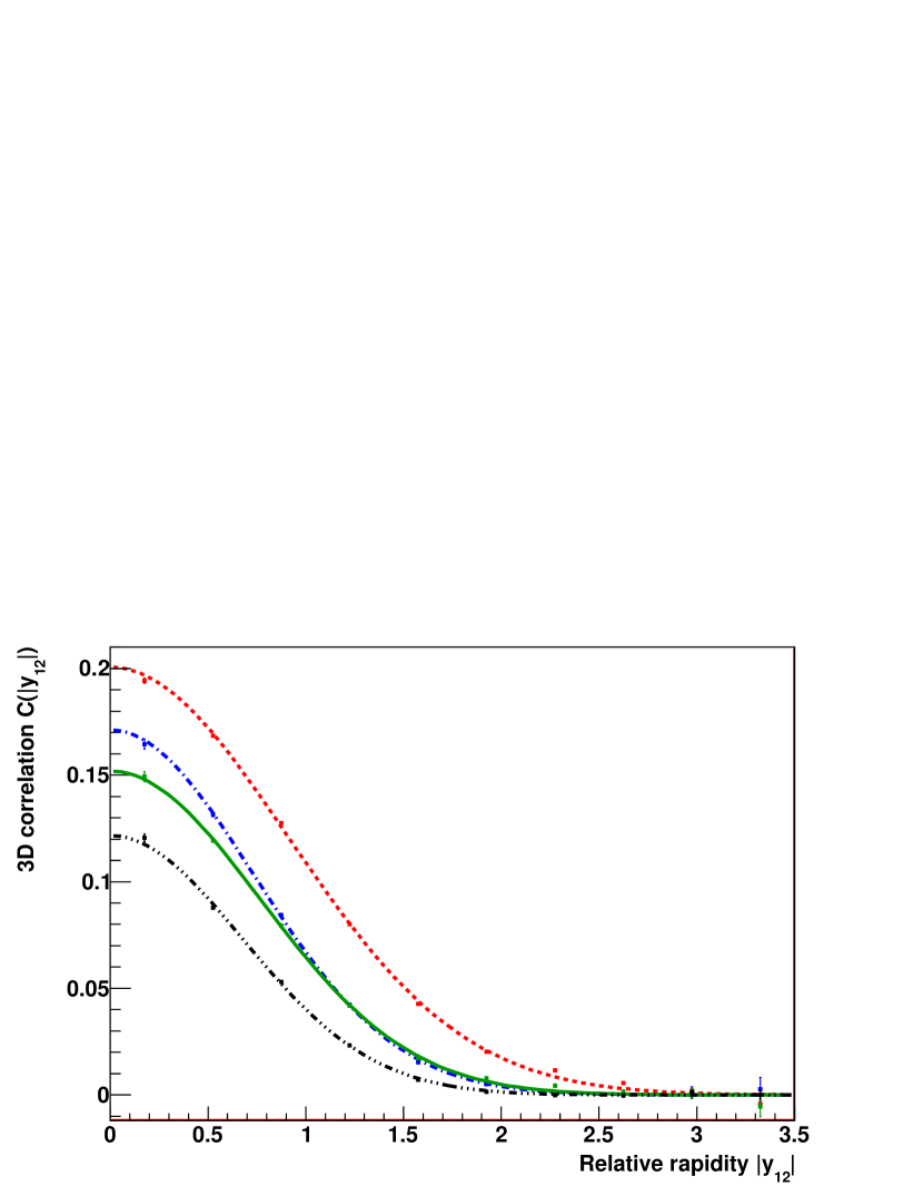
Figure 6: Comparison of correlation functions in $y_{12}$ for different collision energies. For parameter sets see text. All hadrons are emitted from droplets with $b=50\,\mbox{fm}^{3}$. Different curves show: FAIR (red dotted curve), RHIC (blue dash-dotted), RHIC without resonances in the simulation (green solid), LHC (black dash-dot-dotted).

a comparison of the correlation functions at different collision energies. The amplitude of the correlation function is highest for FAIR. This is due to the regime with lowest average $dN/dy$ where clusterization in momentum space is best visible. Somewhat surprising, the FAIR correlation function is also the widest. We expected just the opposite since the kinetic freeze-out energy at FAIR was lower than in the other two cases. The larger width of the correlation function is caused by the Gaussian profile of the fireball in space time rapidity in comparison with uniform profiles at higher energies. Again, we can understand the effect to some extent from eq.(19): a source with narrow rapidity distribution will have smaller $\xi$. This broadens the peak of the Gaussian correlation function. Paradoxically, fireball that is very narrow in space-time rapidity will have wide correlation function.

5 Conclusions

Correlation functions in relative rapidity appear to be a powerful tool for the study of clustering of hadron production due to fragmentation. Note that in calculating the correlation functions we did not include the effect of final state interaction (strong and Coulomb) between the protons pratt94 , which governs the correlation function in absence of other effects. This method was also followed in randrup05 . Hence, our results cannot be directly compared to experimental data and should be regarded as an estimate of the size of the effect. It is large indeed, if the droplets have average volume of few tens of fm³. With the average size reaching down to the level of a few fm³ the influence on the correlation function is on the per cent level. This is the size of the droplets which may be expected at RHIC, as indicated by data from PHOBOS. At the LHC, the droplets, if any, are likely to be smaller Torrieri:2007fb .

This study assumed that after emission from the droplets, hadrons do not rescatter. Rescattering would weaken the correlation and might even wash it away.

Also, note that we did not study correlation of three and more protons randrup05 . Such correlations demand much better statistics and are small if the average volume of droplets drops considerably below 10 fm³. For such small droplets it becomes unlikely that more than two protons will be emitted from one droplet. Note that we do not expect at RHIC droplets much bigger than this (if any). Thus two-particle correlation appears to be the most suitable tool at these collision energies.

Acknowledgements

We gratefully acknowledge financial support by grants No. MSM 6840770039, and LC 07048 (Czech Republic). BT also acknowledges support from VEGA 1/4012/07 (Slovakia).

References

- (1) Y. Aoki, G. Endrodi, Z. Fodor, S. D. Katz and K. K. Szabo, Nature 443 (2006) 675 [arXiv:hep-lat/0611014].
- (2) M. A. Stephanov, Prog. Theor. Phys. Suppl. 153 (2004) 139 [Int. J. Mod. Phys. A 20 (2005) 4387] [arXiv:hep-ph/0402115].
- (3) Z. Fodor and S. D. Katz, JHEP 0404 (2004) 050 [arXiv:hep-lat/0402006].
- (4) L. P. Csernai and I. N. Mishustin, Phys. Rev. Lett. 74 (1995) 5005.
- (5) I. N. Mishustin, Phys. Rev. Lett. 82 (1999) 4779 [arXiv:hep-ph/9811307].
- (6) I. N. Mishustin, Nucl. Phys. A 681 (2001) 56.
- (7) O. Scavenius, A. Dumitru, E. S. Fraga, J. T. Lenaghan and A. D. Jackson, Phys. Rev. D 63 (2001) 116003 [arXiv:hep-ph/0009171].
- (8) K. Paech and S. Pratt, Phys. Rev. C 74, 014901 (2006) [arXiv:nucl-th/0604008].
- (9) D. Kharzeev and K. Tuchin, JHEP 0809, 093 (2008) [arXiv:0705.4280 [hep-ph]].
- (10) H. B. Meyer, Phys. Rev. Lett. 100 (2008) 162001 [arXiv:0710.3717 [hep-lat]].
- (11) G. Torrieri, B. Tomášik and I. Mishustin, Phys. Rev. C 77 (2008) 034903 [arXiv:0707.4405 [nucl-th]].
- (12) G. Torrieri and I. Mishustin, Phys. Rev. C 78 (2008) 021901 [arXiv:0805.0442 [hep-ph]].
- (13) K. Rajagopal and N. Tripuraneni, arXiv:0908.1785 [hep-ph].
- (14) S. Pratt, Phys. Rev. C 49 (1994) 2722.
- (15) J. Randrup, Heavy Ion Physics 22 (2005) 69.
- (16) B. Tomášik, Comp. Phys. Commun. 180 (2009) 1642 [arXiv:0806.4770 [nucl-th]]
- (17) F. Becattini, M. Gaździcki, A. Keränen, J. Manninen and R. Stock, Phys. Rev. C 69 (2004) 024905 [arXiv:hep-ph/0310049].