Symmetry breaking in a localized interacting binary BEC in a bi-chromatic optical lattice

Abstract

By direct numerical simulation of the time-dependent Gross-Pitaevskii equation using the split-step Fourier spectral method we study different aspects of the localization of a cigar-shaped interacting binary (two-component) Bose-Einstein condensate (BEC) in a one-dimensional bi-chromatic quasi-periodic optical-lattice potential, as used in a recent experiment on the localization of a BEC [Roati et al., Nature 453, 895 (2008)]. We consider two types of localized states: (i) when both localized components have a maximum of density at the origin $x=0$, and (ii) when the first component has a maximum of density and the second a minimum of density at $x=0$. In the non-interacting case the density profiles are symmetric around $x=0$. We numerically study the breakdown of this symmetry due to inter-species and intra-species interaction acting on the two components. Where possible, we have compared the numerical results with a time-dependent variational analysis. We also demonstrate the stability of the localized symmetry-broken BEC states under small perturbation.

I Introduction

After the prediction of the localization of the electronic wave function in a disordered potential by Anderson fifty years ago anderson , there have been many studies on different aspects of localization of different types of waves, e.g., electron wave, sound wave, electromagnetic wave, etc light ; micro ; sound , and quantum matter wave in the form of a Bose-Einstein condensate (BEC) billy ; roati ; chabe ; edwards . In the case of a quantum matter wave a disordered speckle potential billy and a quasi-periodic bi-chromatic optical lattice (OL) potential roati have been employed for the localization of a non-interacting cigar-shaped BEC. The quasi-periodic bi-chromatic OL potential was formed by the superposition of two standing-wave polarized laser beams with incommensurate wavelengths. Each standing-wave polarized laser beam leads to a periodic OL potential. The non-interacting BEC of ³⁹K atoms was created roati by tuning the inter-atomic scattering length to zero near a Feshbach resonance fesh .

The localization of a cigar-shaped BEC in a one-dimensional (1D) bi-chromatic OL potential and related topics have been the subject matter of several theoretical das ; dnlse ; boers ; random ; optical ; modugno ; roux ; roscilde ; paul ; adhikari and experimental billy ; roati ; chabe ; edwards studies. (Localized BEC states in the form of gap soliton in a mono-chromatic OL potential have also been observed gsexp and studied gs . However, there are fundamental differences between the two types of localized states. The Anderson localized states in bi-chromatic OL potential appear predominantly in the linear Schrödiger equation and are destroyed above a small critical repulsive nonlinearity, whereas the gap solitons appear only in the presence of a repulsive nonlinearity. The linear system does not support a localized gap soliton. The gap solitons appear in the band gap of the spectrum of the periodic OL potential. On the other hand, the potential supporting the Anderson states must be aperiodic in nature.) After the pioneering experiments [5, 6] on the localization of a 1D cigar-shaped non-interacting BEC, a natural extension of this phenomenon would be to investigate localization in a weakly-interacting binary (two-component) BEC mixture.

In this paper, with intensive numerical simulations of the Gross-Pitaevskii (GP) equation, we study different aspects of localization of a cigar-shaped binary BEC in a 1D bi-chromatic quasi-periodic OL potential $-$ similar to the one used in the experiment of Roati et al. roati . Although, most of the studies of Anderson localization were confined to non-interacting systems, in the present study on the localization of a two-component BEC we shall mostly consider a weakly-interacting system under the action of both inter-species and intra-species interaction. If the potential $V(x)$ is symmetric around origin at $x=0$, e.g. $V(x)=V(-x)$, for the non-interacting system the density profiles are symmetric around $x=0$: $|u(x)|^{2}=|u(-x)|^{2},$ where $u(x)$ is the wave function of the matter wave. But for the interacting system with inter- and intra-species interaction, this symmetry can be broken and different types of symmetry-broken states emerge and we shall be specially interested in the study of the formation of localized cigar-shaped BEC components with broken symmetry.

The two components of the BEC could be two different hyperfine states of the same atom binary1 or two different atoms binary2 and the two confining bi-chromatic OL potential for the two components could be the same or different adhikari ; modugno ; roati . The bi-chromatic OL potential could be taken as the linear combination of two sine terms, both with a minimum at the origin ($x=0$), when the confined BEC components will have a maximum at the origin. The bi-chromatic OL potential could also be taken as the linear combination of two cosine terms with a maximum at the origin, while the confined BEC components will have a minimum at the origin. We shall consider two distinct situations of localized binary BEC: (i) two components under the action of the identical sine bi-chromatic OL potential while both densities have maxima at $x=0$, and (ii) component 1 under the action of the sine bi-chromatic OL potential with a maximum of density at $x=0$ and component 2 under the action of the cosine bi-chromatic OL potential with a minimum of density at $x=0$. In case (i) with weak inter-species and intra-species repulsions, the localized BEC components are overlapping with a maximum at $x=0$. But under the action of a inter-species repulsion above a critical value, the two repealing BEC components separate and move to opposite sides of $x=0$, thus breaking the symmetry around $x=0$. It is this separation or splitting of the BEC components which we study. (Similar separation of gap solitons gs in a binary BEC mixture confined by a monochromatic lattice has been studied malomed ; malomed2 .) In case (ii) a different type of symmetry breaking emerges. In this case with weak intra-species and inter-species repulsion or attraction, the localized BEC components have densities symmetric around $x=0$. But under the action of an inter-species attraction above a critical value, the two attracting BEC components try to stick together as a pair of bright solitons cpld and the minimum-energy stable configuration is the one where both components move predominantly to the same side of $x=0$, thus breaking the symmetry around $x=0$. We study this symmetry breaking in details. In our study we use direct numerical simulation of the underlying GP equation using the split-step Fourier spectral method. We also use a time-dependent variational analysis for an analytical understanding of the numerical results in case (i) above when both components have a maximum at $x=0$ with densities having quasi-Gaussian shapes. In this case certain aspects of the splitting of the two components are also predicted correctly from the variational analysis.

There have already been a number of theoretical and experimental studies on Anderson localization in different problems. The effect of a repulsive non-linearity on localization of light waves in photonic crystals was studied experimentally lahini . There have also been studies of a weak repulsion on localization dnlse ; modugno ; adhikari ; interaction . Damski et al. and Schulte et al. considered Anderson localization in disordered OL potential optical whereas Sanchez-Palencia et al. and Clément et al. considered Anderson localization in a random potential random . There have been studies of Anderson localization with other types of disorder other . Anderson localization in BEC under the action of a disordered potential in two and three dimensions has also been investigated 2D3D .

In Sec. II we present a brief account of (i) the two-component 1D GP equation, (ii) the bi-chromatic OL potentials used in our study and (iii) a time-dependent variational analysis of the GP equation under appropriate conditions. In Sec. III we present our numerical studies on localization using the split-step Fourier spectral method. The density profile of the quasi-Gaussian localized states are in agreement with the variational results. The density of the localized states are symmetric around the origin at $x=0$ in the absence of inter-species interaction. We study the symmetry breaking under the action of an inter-species interaction. Certain aspects of symmetry breaking can be explained with the variational analysis. We demonstrate the dynamical stability of the two-component localized states. In Sec. IV we present a brief discussion and concluding remarks.

II Analytical consideration of localization

We consider a two-component cigar-shaped BEC under tight transverse harmonic confinement with the bi-chromatic OL potential acting along the axial $x$ direction. Then it is appropriate to consider a 1D reduction 1d of the 3D GP equation by freezing the transverse dynamics to the respective ground state and integrating over the transverse variables. Such a binary BEC is described by the following coupled 1D BEC equation 1d ; malomed :

$$i\frac{\partial u_{1}}{\partial t}=-\frac{1}{2}\frac{\partial^{2}u_{1}}{\partial x^{2}}+g_{1}|u_{1}|^{2}+g_{12}|u_{2}|^{2}u_{1}+V_{1}(x)u_{1},$$ (1)

$$i\frac{\partial u_{2}}{\partial t}=-\frac{1}{2}\frac{\partial^{2}u_{2}}{\partial x^{2}}+g_{2}|u_{2}|^{2}+g_{12}|u_{1}|^{2}u_{2}+V_{2}(x)u_{2},$$ (2)

with normalization $\int_{-\infty}^{\infty}|u_{j}|^{2}dx=1,$ of the localized wave function $u_{j}$ of the two components $j=1,2$. As the localization of the BEC in the bi-chromatic lattice is most prominent for the linear problem, and we shall be interested in small non-linearities $g_{1},g_{2}$ and $g_{12}$. To make the parameters of the model tractable we take the number of atoms $N_{j}$ and the mass $m_{j}$ of the two components to be equal: $N_{1}=N_{2}=N$ and $m_{1}=m_{2}=m$. This simplification will have no effect on the general conclusion of this study. The intra-species nonlinearities are given by 1d $g_{j}=2a_{j}N/a_{\perp},a_{\perp}\equiv\sqrt{\hbar/(m\omega)},\omega\equiv\sqrt{\omega_{y}\omega_{z}}$ where $\omega_{y}$ and $\omega_{z}$ are the transverse trap frequencies in the $y$ and $z$ directions, respectively, and $a_{j}$ is the intra-species atomic scattering length. The inter-species non-linearity is given by 1d $g_{12}=2Na_{12}/a_{\perp}$, where $a_{12}$ is the inter-species scattering length. In Eqs. (1) and (2) $V_{j}(x)$ are the bi-chromatic OL traps of the two components $j=1,2$. Here we are using harmonic oscillator units: length is expressed in units of transverse oscillator length $a_{\perp}$ and time in units of angular frequency $(\omega)^{-1}$.

In the first part of our study we shall take the two bi-chromatic OL potentials to be identical $-$ $V_{1}(x)=V_{2}(x)=V(x)$ $-$ and have the following sine form as in the experiment roati

$$V(x)=\sum_{l=1}^{2}A_{l}\sin^{2}(k_{l}x),$$ (3)

with $A_{l}=2\pi^{2}s_{l}/\lambda_{l}^{2}$, where $\lambda_{l}$’s are the wavelengths of the laser forming the OL potentials, $s_{l}$’s are their intensities, and $k_{l}=2\pi/\lambda_{l}$ the corresponding wave number. In the second part of our study we shall take $V_{1}(x)$ to be given by Eq. (3) whereas in $V_{2}(x)$ the sine term is replaced by a cosine term:

$$V_{2}(x)=\sum_{l=1}^{2}A_{l}\cos^{2}(k_{l}x),$$ (4)

Potentials (3) and (4) are quite similar. However, potential (4) generates a different type of localized states compared to potential (3). Potential (3) has a local minimum at the center $x=0$; consequently, stable stationary solutions with this potential have a maximum at $x=0$. However, potential (4) has a local maximum at $x=0$ corresponding to a minimum of the stationary solution at the center.

With a single periodic potential of the form $\sin^{2}(2\pi x/\lambda)$ or $\cos^{2}(2\pi x/\lambda)$ with $s_{2}=0,$ the linear Schrödinger equation permits only de-localized states in the form of Bloch waves. Localization is possible in the linear Schrödinger equation due to the “disorder” introduced through a second component in Eqs. (3) or (4). The primary lattice is usually strong enough and is used as the main periodic potential fixing the Bloch band structure of the single-particle states without disorder. The secondary lattice is weaker ($s_{2}<<s_{1}$) and introduces a “deterministic” disorder. Following the experiment of Roati et al. roati , the transverse harmonic-oscillator length is of the order of a few microns so that the wavelengths of the OL in dimensionless units become approximately $10^{0}\sim 10^{1}$.

Usually, the stationary BEC localized states formed with bi-chromatic lattices occupy many sites of the quasi-periodic OL potential and their shape is modulated by the short-wavelength potential bishop . For certain values of the parameters, potential (3) leads to bound states confined practically to the central site of the quasi-periodic OL potential. When this happens, a variational approximation with Gaussian ansatz leads to a reasonable prediction for the bound state. To apply the variational approach with potential (3) effective on both components, we adopt the Gaussian function below as the variational ansatz PG

$$u_{j}(x,t) = \frac{1}{\pi^{1/4}}\sqrt{\frac{{\cal N}_{j}}{w_{j}}}\exp[-(x-x_{0j})^{2}/(2w_{j}^{2})]$$ (5)

$$\times \exp[i\{C_{j}(x-x_{0j})+\phi_{j}\}],$$

where $w_{j}$ are the widths of component $j$ of localized BEC centered at $x_{0j}$, $\phi_{j}$ is the corresponding phase, $C_{j}$ is the linear phase coefficient and ${\cal N}_{j}$ is the normalization of component $j$. We shall consider solution where the widths are comparable to the OL wavelength. Generally, the variational approach is valid when the OL is only smooth and slowly varying on the localized states scale bishop . We shall obtain useful relations among the variational parameters of the localized BEC states. This will allow us to get a better physical understanding of the localized states.

The GP equations (1) and (2) can be derived from the following Lagrangian

$$L(t) = \int_{-\infty}^{\infty}\biggr{[}\sum_{j=1}^{2}\biggr{(}\frac{i}{2}[u_{j}^{*}\dot{u}_{j}-u_{j}\dot{u}^{*}_{j}]-\frac{1}{2}[|u^{\prime}_{j}|^{2}+g_{j}|u_{j}|^{4}]$$ (6)

$$- V(x)|u_{j}|^{2}\biggr{)}-g_{12}|u_{1}|^{2}|u_{2}|^{2}\biggr{]}dx,$$

where the overhead dot denotes time derivative, the star denotes complex conjugation, and the prime denotes space derivative. Using ansatz (5) in Eq. (6) we get

$$L(t) = \sum_{j=1}^{2}{\cal N}_{j}\biggr{[}(C_{j}\dot{x}_{0j}-\dot{\phi}_{j})-\frac{1}{2}\left(\frac{1}{2w_{j}^{2}}+C_{j}^{2}\right)$$

$$- \frac{g_{j}{\cal N}_{j}}{2\sqrt{2\pi}w_{j}}+\sum_{l=1}^{2}L_{lj}\biggr{]}+L_{12},$$

$$L_{12} \equiv -\int_{-\infty}^{\infty}g_{12}|u_{1}|^{2}|u_{2}|^{2}dx$$ (8)

$$= -\frac{g_{12}{\cal N}_{1}{\cal N}_{2}}{\sqrt{\pi(w_{1}^{2}+w_{2}^{2})}}\exp\left[-\frac{\rho^{2}}{w_{1}^{2}+w_{2}^{2}}\right],$$

$$L_{lj} \equiv \frac{A_{l}}{2}\left[\cos(2k_{l}x_{0j})\exp(-k_{l}^{2}w_{j}^{2})-1\right]$$ (9)

where $\rho=x_{02}-x_{01},$ and the variational parameters are the norm ${\cal N}_{j}$, width $w_{j}$, position $x_{0j}$, and phase parameters $C_{j}$ and $\phi_{j}$. We use the Euler-Lagrange equation

$$\frac{\partial L}{\partial\sigma}-\frac{d}{dt}\frac{\partial L}{\partial\dot{\sigma}}=0,$$ (10)

where $\sigma$ is the variational parameter. The first variational equation using $\sigma=\phi_{j}$ yields ${\cal N}_{j}=$ constant. Without losing generality we shall take this constant to be unity and use it in the subsequent equations. Taking $\sigma=x_{0j},C_{j},w_{j},$ and ${\cal N}_{j},$ respectively, we obtain the following equations

$$\dot{C}_{j} = \frac{\partial}{\partial x_{0j}}\left[\sum_{l=1}^{2}L_{lj}+L_{12}\right],$$ (11)

$$\dot{x}_{0j} = C_{j},$$ (12)

$$\frac{1}{w_{j}} + \frac{g_{j}}{\sqrt{2\pi}}+\frac{2g_{12}w_{j}^{3}}{\sqrt{\pi}(w_{1}^{2}+w_{2}^{2})^{3/2}}\left[1-\frac{2\rho^{2}}{w_{1}^{2}+w_{2}^{2}}\right]$$ (13)

$$\times \exp\left[-\frac{\rho^{2}}{w_{1}^{2}+w_{2}^{2}}\right]-\sum_{l=1}^{2}2A_{l}w_{j}^{3}k_{l}^{2}\cos(2k_{l}x_{0j})$$

$$\times \exp(-k_{l}^{2}w_{j}^{2})=0,$$

$$\dot{\phi}_{j} = \frac{C_{j}^{2}}{2}-\frac{1}{4w_{j}^{2}}-\frac{g_{j}}{w_{j}\sqrt{2\pi}}+\frac{\partial L_{12}}{\partial{\cal N}_{j}}\biggr{|}_{{\cal N}_{j}=1}+\sum_{l=1}^{2}L_{lj}.$$

The set of equations (11) $-$ (II) shows that the phase $\phi_{j}$ has no effect on the location $x_{0j}$, width $w_{j}$ and the coefficient $C_{j}$ of solitons, whereas it is determined by the variational equation (II). Hence we shall neglect Eq. (II) in the following and consider only Eqs. (11) $-$ (13). (However, we could not set phase $\phi_{j}=0$ in the beginning, as the Euler-Lagrange equation for $\phi_{j}$ leads to the important result of norm conservation.) Equation (13) determines the width $w_{j}$ in terms of nonlinearities $g_{j}$, $g_{12}$ and the parameters of the bi-chromatic OL potential. The density distribution is quasi-Gaussian only for small values of $x_{0j}$, and we shall be limited to this constraint (small $|x_{0j}|$) while considering the variational approach. In the symmetric case, while $g_{1}=g_{2}$, the widths of the two localized states are equal. However, when $g_{1}\neq g_{2}$, the widths of the two localized states are not equal and one has two asymmetric localized states. When $x_{01}=x_{02}=0$, the widths of the two stationary BEC localized states are determined by

$$\frac{1}{w_{j}} + \frac{g_{j}}{\sqrt{2\pi}}+\frac{2g_{12}w_{j}^{3}}{\sqrt{\pi}(w_{1}^{2}+w_{2}^{2})^{3/2}}$$ (15)

$$- \sum_{l=1}^{2}2A_{l}w_{j}^{3}k_{l}^{2}\exp(-k_{l}^{2}w_{j}^{2})=0.$$

Now we obtain, following Ref. cheng , the equation of motion describing the center of the two BEC localized states as if they were a particle in an effective potential. Thus, we can determine the motion of equivalent particles using the classical mechanics analogy. Inserting Eqs. (8), (9) and (11) into Eq. (12), we obtain the following equation for dynamics

$$\frac{d^{2}x_{0j}}{dt^{2}} = -\frac{\partial V_{\mathrm{eff}j}}{\partial x_{0j}}\;,$$ (16)

$$V_{\mathrm{eff}j} = \frac{g_{12}}{\sqrt{\pi(w_{1}^{2}+w_{2}^{2})}}\exp\left[-\frac{\rho^{2}}{w_{1}^{2}+w_{2}^{2}}\right]$$ (17)

$$- \sum_{l=1}^{2}\frac{A_{l}}{2}[\cos(2k_{l}x_{0j})\exp(-k_{l}^{2}w_{j}^{2})-1]\;,$$

where the an-harmonic effective potentials $V_{\mathrm{eff}j}$ are the dynamic potentials for the movement of the center of the localized BECs and depend on characteristics of the two BEC localized states (e.g., width $w_{j}$ and position $x_{0j}$) and potential parameters (e.g., $k_{l}$ and $A_{l}$). The effective potentials have two parts. The first term on the right of Eq. (17) is induced by the mutual interaction of the two BEC localized states. When the coupling constant $g_{12}>0$, it is positive and contributes to a repulsive potential barrier for BEC localized states. The second term in Eq. (17) arises from the bi-chromatic OL potential and contributes to an attractive potential well, if $|x_{0j}|$ is small enough. The combination of the two terms may lead to local minima or local maxima at the origin $x_{0j}=0$ in the effective potential $V_{\mathrm{eff}j}$.

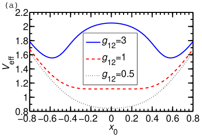
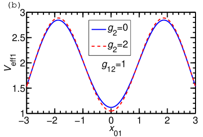
(a)                           (b)

Figure 1: (Color online) (a) The effective potential $V_{\mathrm{eff}}(x_{0})$ vs. the position of the localized state $x_{0}\equiv x_{01}=-x_{02}$ in the symmetric case $g_{1}=g_{2}=0$ for $g_{12}=0.5,1$ and 3 as obtained from Eq. (17). The respective widths are calculated from Eq. (13). (b) The effective potential felt by the first component $V_{\mathrm{eff}1}(x_{01})$ vs. its position $x_{01}$ as obtained from Eq. (17). The widths of the two states are calculated from Eq. (15). In both cases $-$ (a) and (b) $-$ the potential parameters are $\lambda_{1}=8,\lambda_{2}=0.862\lambda_{1},s_{1}=8,s_{2}=2.4.$

When the two BEC localized states are symmetrical $(g_{1}=g_{2})$, they will feel the same effective potential. In that case, we should have $w_{1}=w_{2}=w$ and $x_{01}=-x_{02}=x_{0}$. The effective potential $V_{\mathrm{eff}}$ is plotted in Fig. 1 (a) vs. $x_{0}$ in the symmetric case $g_{1}=g_{2}=0$ for different inter-species interaction: $g_{12}=0.5,1,$ and 3. Equation (13) is first solved to find $w$ as a function of $x_{0}$. This result is then substituted in Eq. (17) to find $V_{\mathrm{eff}}(x_{0})$ as plotted in Fig. 1 (a). From Fig. 1 (a) we find that if $g_{12}$ is smaller, the effective potential possesses a local minimum at $x_{0}=0$. In this case if we start with two BEC localized states at $x=0$ for small $g_{12}$, they will be in stable equilibrium and unsplit. The effective potential becomes weaker with the local minimum at $x_{0}=0$ less pronounced as $g_{12}$ increases. If $g_{12}$ is large enough (e.g., $g_{12}=3$ in Fig. 1 (a)), a local maximum appears in the effective potential at $x_{0}=0$; and the peak value at maximum increases as $g_{12}$ increases. In this case two overlapping (unsplit) initial localized BEC states at the maximum at $x=0$ will be in a metastable configuration. When they are slightly perturbed, for example, by slightly moving the BEC center(s) from $x=0$, they will move respectively toward the minima of the effective potential next to the maximum and split into two non-overlapping BECs localized at the two local minima of the effective potential on both sides of $x_{0}=0$ as we shall see in Sec. III.1.

When the two BEC localized states are asymmetrical ($g_{1}\neq g_{2}$), they will feel different effective potentials. It is difficult to calculate these effective potentials exactly. But we can calculate the effective potential(s) (17) under simplifying assumptions. The widths $w_{1}$ and $w_{2}$ are assumed to be independent of positions $x_{01}$ and $x_{02}$ and were calculated using Eq. (15) and substituted into Eq. (17). The function $V_{\mathrm{eff}1}(x_{01})$ so obtained is plotted in Fig. (1) (b) vs. $x_{01}$, for $g_{1}=0,g_{12}=1,g_{2}=0$ and 2. The effective potential acting on component 1 is stronger as $g_{2}$ is increased from 0 to 2. This will lead to a reduction of the width of the corresponding localized state as $g_{2}$ is increased from 0 to 2 as we shall see in Sec. III.1.

III Numerical Results

We perform the numerical simulation employing the real-time split-step Fourier spectral method with space step 0.04, time step 0.001. (We also checked the results using the real-time Crank-Nicolson discretization routine, the FORTRAN programs which are given in Ref. bo1 .) Because of the oscillating nature of the potential, great care was needed to obtain a precise localized state. The accuracy of the numerical simulation was tested by varying the space and time steps as well as the total number of space steps. The initial input pulse is a Gaussian wave packet, $u_{j}(x,t=0)=\pi^{-1/4}\exp(-x^{2}/2)$ with a parabolic trap $V^{\prime}(x)=x^{2}/2$. Let $g_{1}=g_{2}=g_{12}=0$ and the coupled Eqs. (1) and (2) become the linear Schrödinger equation. To start the numerical simulation the parabolic trap is slowly turned off and the bi-chromatic OL is slowly turned on; the increment in the coefficient $s_{i}$ in each time step is 0.00005. Successively, we add gradually the nonlinear coefficient $g_{2}$ and the coupling constant $g_{12}$ slowly. The increment of $g_{2}$ and $g_{12}$ is 0.00001 in each time step. Thereby the stationary localized states are obtained.

To perform a systematic numerical study of localization we take $s_{1}=8$, $s_{2}=2.4$, $\lambda_{1}=8$ and $\lambda_{2}=0.862\lambda_{1}$ maintaining the ratio $\lambda_{2}/\lambda_{1}=0.862$ similar to the value employed in the experiment roati . The values of $s_{1}$ and $s_{2}$ are also in the range employed in the experiment. With these set of parameters and for weak inter-species and intra-species interactions, the localized BEC state could be mostly confined in the single cell of the bi-chromatic OL potential. All results reported here are obtained with these potential parameters except those in Figs. 3 (e) and (f) where we study the effect of the change of potential parameters. We consider a transverse harmonic oscillator length $a_{\perp}\approx 1$ $\mu$m, so that the wave lengths of the OL potential are approximately $800$ nm and $689$ nm. We shall take $g_{1}=0$ throughout the present investigation.

III.1 Localized states with potential (3) on both components

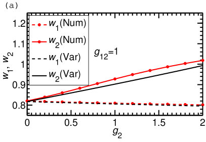
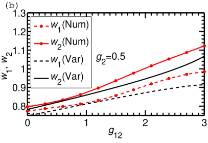
(a)                           (b)

Figure 2: (Color online) (a) The numerical and variational widths $w_{1}$ and $w_{2}$ of the two stationary BEC localized states vs. $g_{2}$ for $g_{12}=1,g_{1}=0$. (b) The same as in (a) vs. $g_{12}$ for $g_{2}=0.5,g_{1}=0$. The potential (3) acts on the two components where the parameters are $\lambda_{1}=8,\lambda_{2}=0.862\lambda_{1},s_{1}=8,s_{2}=2.4$.

We start the numerical analysis with a consideration of the widths of the two components of the localized BECs with potential (3) acting on both components. In this case both the components could have a maximum at the center $x=0$ with localized states of quasi-Gaussian forms and when this happens the system can be described well by the variational approximation. Assuming a Gaussian distribution for the localized BEC, the numerical width is calculated via

$$w_{j}^{2}=2\int_{-\infty}^{\infty}|u_{j}|^{2}x^{2}dx.$$ (18)

The numerical and variational results for the widths $w_{j}$ vs. $g_{2}$ for $g_{12}=1$ are plotted in Fig. 2 (a). The same for $g_{2}=0.5$ vs. $g_{12}$ are plotted in Fig. 2 (b). In these plots there is reasonable agreement between the numerical and variational results for the width and the width usually increases with the increase of nonlinearities $g_{2}$ and $g_{12}$ except in the case of $w_{1}$ in Fig. 2 (a). The general increase of width with the increase of non-linearity (increase of repulsion) is expected, however, the decrease of $w_{1}$ with $g_{2}$ in Fig. 2 (a) requires special attention. This phenomenon will be clear if we consider the effective potential of component 1 as illustrated in Fig. 1 (b) when $g_{2}$ is changed from 0 to 2. We find that the effective potential becomes slightly stronger as $g_{2}$ increases corresponding to a reduction of width $w_{1}$ in Fig. 2 (a) with the increase of $g_{2}$.

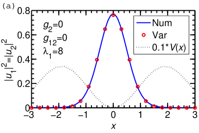
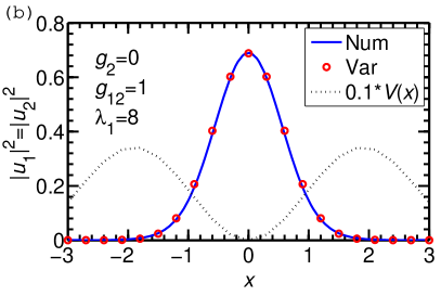
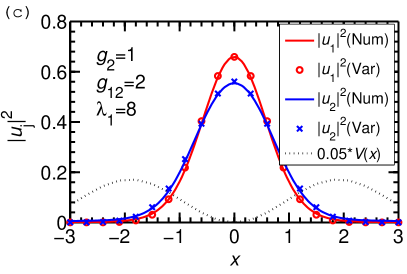
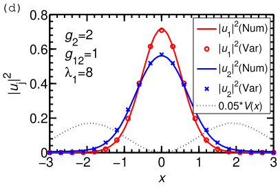
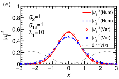
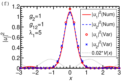
(a)                           (b)                            (c)                           (d)                            (e)                           (f)

Figure 3: (Color online) The densities $|u_{1}(x)|^{2}$ and $|u_{2}(x)|^{2}$ of the two localized BEC states vs. $x$ for (a) $g_{1}=g_{2}=g_{12}=0$; (b) $g_{1}=g_{2}=0$ and $g_{12}=1$; (c) $g_{1}=0,g_{2}=1,$ and $g_{12}=2$; (d) $g_{1}=0,g_{2}=2,$ and $g_{12}=1$. In (a), (b), (c), and (d) potential (3) acts on the two components with parameters $\lambda_{1}=8,\lambda_{2}=0.862\lambda_{1},s_{1}=8,s_{2}=2.4.$ The same as in (a) for $g_{1}=0,g_{2}=g_{12}=1$ with potential parameters (e) $\lambda_{1}=10,\lambda_{2}=0.862\lambda_{1},s_{1}=8,s_{2}=2.4$ and (f) $\lambda_{1}=5,\lambda_{2}=0.862\lambda_{1},s_{1}=8,s_{2}=2.4.$ In each case the profile of the bi-chromatic OL potential is also shown.

Next we consider typical numerical profiles of the density of the localized BEC states $|u_{j}|^{2}$ and compare them with variational results for small values of $g_{12}$ when the centers of both components are at the origin: $x_{01}=x_{02}=0$. In Figs. 3 (a) and (b) we present the results for $g_{1}=g_{2}=0$ and $g_{12}=0$ and 1, respectively, while the two density profiles $|u_{1}|^{2}$ and $|u_{2}|^{2}$ are equal. Next we consider results for the asymmetric case while $g_{1}\neq g_{2}$ while the two densities are different. In Figs. 3 (c) and (d) we present the results for $g_{1}=0,g_{2}=1,g_{12}=2$ and for $g_{1}=0,g_{2}=2,g_{12}=1$, respectively. In both cases the component 1 is more strongly localized in space with a smaller width. Next we consider the effect of a variation of the wavelengths $\lambda_{1}$ and $\lambda_{2}$ on the densities. In Fig. 3 (e) we plot the densities for $\lambda_{1}=10,\lambda_{2}=0.862\lambda_{1}$, and in Fig. 3 (f) we plot the densities for $\lambda_{1}=5,\lambda_{2}=0.862\lambda_{1}$; in both cases we take $g_{1}=0,g_{2}=g_{12}=1,s_{1}=8,s_{2}=2.4.$ In Fig. 3 (e) with the increase of $\lambda$’s the central OL site has a larger spatial extension, consequently the densities have a smaller value at the maxima at the origin corresponding to a larger width. In Fig. 3 (f) with the decrease of $\lambda$’s the central OL site has a smaller spatial extension, consequently the densities have a larger value at the maxima at the origin corresponding to a smaller width. The plots in Figs. 3 (a) $-$ (e) indicate that the numerical results for densities are in perfect agreement with the variational results. It also indicates the good accuracy of the numerical routine. In these cases the density has a quasi-Gaussian profile used in the variational analysis. In Fig. 3 (f) the numerical densities have secondary maxima on both sides of the central peak, and the profile deviates from the Gaussian and the agreement with the variational results in this case is only fair.

So far we presented results in the asymmetric case for small values of $g_{12}$ where the two localized states are overlapping (unsplit) and centered at $x=0$. As $g_{12}$ increases it is clear from Fig. 1 (a) that the effective potentials experienced by the components develop a maximum at the origin. Hence the position $x=0$ ceases to be one of stable equilibrium for the components. Consequently, the two localized BECs move on opposite sides of the point $x=0$ to attain split (separated) configurations of stable equilibrium. We illustrate this in the symmetric case in Fig. 4 (a) for $g_{1}=g_{2}=0,g_{12}=3$ where we plot the densities of the two split components. The two densities continue to be symmetric: $|u_{1}(x)|^{2}=|u_{2}(-x)|^{2}$ with centers at $|x_{01}|=|x_{02}|=0.45$. From Fig. 1 (a) we find that the minima of the effective potential for the same set of parameters as in Fig. 4 (a) are at $|x_{01}|=|x_{02}|=0.58$ indicating the centers of the split solitons to be at $\pm 0.58$. The variational analysis is valid for small splitting, and considering that the value $\pm 0.58$ indicating splitting is not too small compared to the extension of the localized states, the agreement between the numerical displacement 0.45 of the localized state and its variational estimate of 0.58 should be considered satisfactory. In Fig. 4 (b), we present an example of the localized asymmetric split states for $g_{1}=0,g_{2}=0.3,g_{12}=3$, where the two states have different (asymmetric) densities.

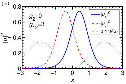
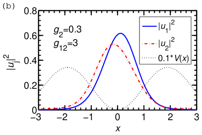
(a)                           (b)

Figure 4: (Color online) (a) The same as in Fig. 3 (a) for (a) $g_{1}=g_{2}=0$ and $g_{12}=3$, and (b) $g_{1}=0,g_{2}=0.3$ and $g_{12}=3.$ The parameters of the potential are $\lambda_{1}=8,\lambda_{2}=0.862\lambda_{1},s_{1}=8,s_{2}=2.4$.

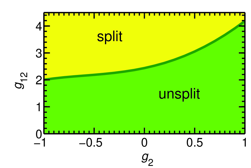
Figure 5: (Color online) The phase diagram of $g_{12}$ vs. $g_{2}$ for $g_{1}=0$ showing the split and unsplit configurations of the two localized states while potential (3) is effective on both components. The parameters of the potential are $\lambda_{1}=8,\lambda_{2}=0.862\lambda_{1},s_{1}=8,s_{2}=2.4$.

As the split and the unsplit configurations of the localized states are of interest, it is appropriate to represent the split and unsplit configurations in a $g_{2}$ vs. $g_{12}$ phase diagram for $g_{1}=0$. This is illustrated in Fig. 5. (Similar split-unsplit phase diagram has also been studied in the context of symbiotic gap solitons malomed .) For small $g_{12}$, as expected, the localized states are in an overlapping (unsplit) configuration. The split configuration is achieved when $g_{12}$ is larger than a critical value indicating a minimum of inter-species repulsion needed to move the localized states from $x=0$. Splitting is favored when the inter-species interaction is strongly repulsive with a large positive value of $g_{12}$ and when the intra-species interaction is attractive corresponding to a negative $g_{2}$ as seen in Fig. 5.

III.2 Localized states with potential (3) on component 1 and potential (4) on component 2

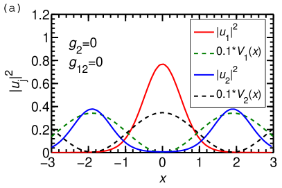
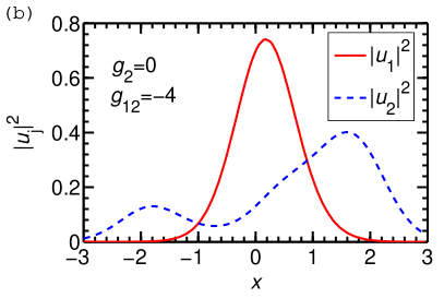
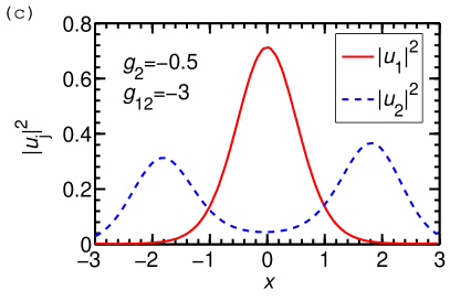
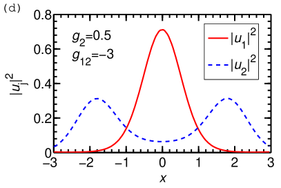
(a)                           (b)                            (c)                           (d)

Figure 6: (Color online) The densities $|u_{1}(x)|^{2}$ and $|u_{2}(x)|^{2}$ of the two localized BEC states vs. $x$ for (a) $g_{1}=g_{2}=g_{12}=0,$ (b) $g_{1}=g_{2}=0,g_{12}=-4$, (c) $g_{1}=0$, $g_{2}=-0.5,g_{12}=-3$, and (d) $g_{1}=0$, $g_{2}=0.5,g_{12}=-3$, when potential (3) acts on the first component and potential (4) acts on the second component. The potential parameters are $\lambda_{1}=8,\lambda_{2}=0.862\lambda_{1},s_{1}=8,s_{2}=2.4.$

Now we consider the situation when potential (3) acts on component 1 and (4) acts on component 2. In this case only the first component under the influence of potential (3) could have a maximum at the origin ($x=0$), and second component under the influence of potential (4) usually has a minimum at the center and hence the variational approximation is not applicable in this case. (The monochromatic counterpart to this model with the phase shifted potential (4) was investigated in Ref. referee .) We start our discussion in this case by showing results of density under different situations. In Fig. 6 (a) we plot the densities of the two components for the symmetric non-interacting case for $g_{1}=g_{2}=g_{12}=0$. The density $|u_{1}|^{2}$ of the first component has a localized Gaussian-type shape centered at $x=0$. The density of the second component has a two-hump symmetric structure with a minimum at $x=0$. The symmetry of the densities around $x=0$ can be broken in the presence of a sufficiently strong inter-species attraction. This is illustrated in Fig. 6 (b) where we plot the densities for $g_{1}=g_{2}=0$ and $g_{12}=-4$. The center of both the densities has moved slightly towards positive $x$ as a sufficiently strong inter-species attraction is introduced via $g_{12}=-4$. In Figs. 6 (c) and (d) we illustrate the densities in two more cases for $g_{1}=0,g_{2}=-0.5,$ and $g_{12}=-3$ and for $g_{1}=0,g_{2}=0.5,$ and $g_{12}=-3$, respectively. In the case of Fig. 6 (c), the densities are asymmetric and in the case of Fig. 6 (d), they are symmetric. This observation is consistent with the general conclusion that the symmetry breaking will be favored when the system is attractive. In the case of Fig. 6 (c) we have $g_{1}=0,g_{2}=-0.5,$ and $g_{12}=-3$ indicating that both components could be bound due to inter-species attraction even in the absence of the bi-chromatic OL potential. Hence due to the inter-species attraction the two localized BEC states tend to overlap and stay together as two bright solitons cpld . In the case represented in Fig. 6 (d) $g_{2}$ is positive and the system is less attractive and hence the density distribution is symmetric.

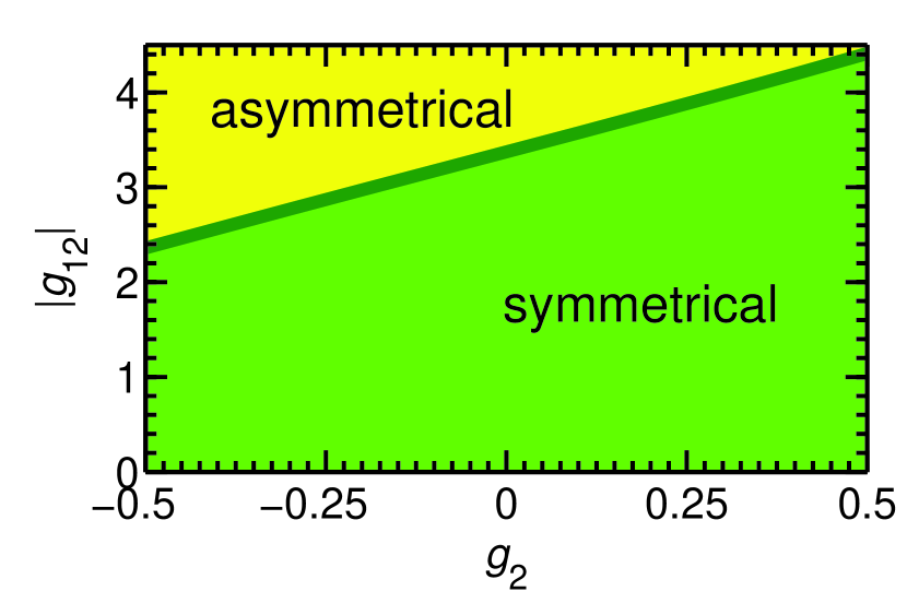
Figure 7: (Color online) The phase diagram of $|g_{12}|$ vs. $g_{2}$ for $g_{1}=0$ showing the symmetric and asymmetric configurations of the two localized BEC states. The potential (3) is effective on the first component and potential (4) on the second component with the same parameters as in Fig. 5.

Again it is worthwhile to show the symmetry breaking in a $g_{2}$ vs. $|g_{12}|$ phase diagram for $g_{1}=0$ as illustrated in Fig. 7. (Similar symmetry breaking has also been studied in the context of symbiotic gap solitons malomed .) For small $|g_{12}|$, as expected, the localized states are in a symmetric configuration. The asymmetric configuration is achieved when $|g_{12}|$ is larger than a critical value indicating that a minimum of attraction is needed to replace the center of the localized states from $x=0$. Symmetry breaking is favored when the inter- and intra-species interactions are strongly attractive leading to strong effective attraction in the system and hence favored for large negative (attractive) values of $g_{2}$ than for positive (repulsive) values of $g_{2}$ as seen in Fig. 7.

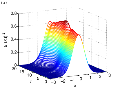
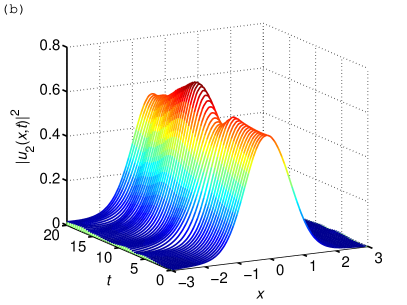
(a)                           (b)

Figure 8: (Color online) The densities (a) $|u_{1}(x,t)|^{2}$ and (b) $|u_{2}(x,t)|^{2}$ vs. $x$ and $t$ of the two localized BEC states of Fig. 4 (b) when the potential parameters are suddenly changed from $\lambda_{1}=8,\lambda_{2}=0.862\lambda_{1},s_{1}=8,s_{2}=2.4$ to $\lambda_{1}=8.5,\lambda_{2}=0.862\lambda_{1},s_{1}=8,s_{2}=2.4$ at time $t=5$.

III.3 The stability of the localized BEC states

So far we studied the stationary properties of the localized BEC states. Now we investigate if the localized BEC states are stable under small perturbation. We are using real-time propagation routines in the numerical calculation, which finds usually the stable states. This indicates that the localized BEC states, we are studying, should be stable. However, we now explicitly demonstrate the stability of a set of specific states, e.g., the ones illustrated in Fig. 4 (b). To demonstrate that these states are stable, after their formation, we suddenly change the potential parameters from $\lambda_{1}=8,\lambda_{2}=0.862\lambda_{1},s_{1}=8,s_{2}=2.4$ to $\lambda_{1}=8.5,\lambda_{2}=0.862\lambda_{1},s_{1}=8,s_{2}=2.4$ and study the resulting dynamics. We plot in Figs. 8 (a) and (b) the consequent density dynamics $|u_{1}(x,t)|^{2}$ and $|u_{2}(x,t)|^{2}$ vs. $x$ and $t$, respectively, for $t=0$ to 20. The sudden change of the potential is effected at $t=5$. From Figs. 8 (a) and (b) we see that at $t=5$ when the potential is suddenly changed the density profiles suffer an abrupt change. Nevertheless, the BEC density profiles remain localized for a large interval of time undergoing breathing oscillation as we can see from Figs. 8 (a) and (b) for the two components, which demonstrates the stability of the localized BEC states.

IV SUMMARY

In this paper, using the numerical and variational solution of the time-dependent GP equation, we studied the localization of two-component cigar-shaped BEC in a quasi-periodic 1D OL potential prepared by two overlapping polarized standing-wave laser beams with different wavelengths and amplitudes. Specifically, we considered two analytical forms (sine and cosine) of the OL potential and considered two distinct cases: (i) the two components under the action of the sine potential (3) and (ii) the sine potential (3) acting on component 1 and the cosine potential (4) acting on component 2. In case (i), for a weak inter-species interaction, both components have a maximum of density at the trap center ($x=0$) satisfying the symmetry $|u_{j}(x)|^{2}=|u_{j}(-x)|^{2}$. In this case the variational analysis is applicable and produced result in good agreement with numerical simulation. In case (ii), for a weak inter-species interaction, one component has a maximum of density at the trap center and the other component has a minimum, however, again satisfying the symmetry $|u_{j}(x)|^{2}=|u_{j}(-x)|^{2}$. The localization is most favored for non-interacting atoms and is destroyed in the presence of moderate intra-species and inter-species repulsive interactions. Here we specially study the effect of weak inter-species and intra-species nonlinearities on the profile of the localized states. In case (i), for a sufficiently strong inter-species repulsion, the two localized states are found to move in opposite directions from the trap center and attain equilibrium in a separated (split) configuration breaking the symmetry $|u_{j}(x)|^{2}=|u_{j}(-x)|^{2}$. In case (ii), for a sufficiently strong inter-species attraction, the two localized states are found to move away from $x=0$ to the same side of the trap center again breaking the symmetry $|u_{j}(x)|^{2}=|u_{j}(-x)|^{2}$. We studied in some detail the formation of the localized states of broken symmetry in all cases considering phase diagram of intra- and inter-species nonlinearities $g_{2}$ and $g_{12}$.

The Anderson localization of a BEC in a bi-chromatic OL potential as studied here is very distinct from the localization of gap solitons gsexp ; gs ; referee of the BEC in a mono-chromatic OL potential. Anderson localization takes place in an aperiodic potential in the linear equation, whereas a periodic potential and a repulsive nonlinearity are crucial for the localization of gap solitons.

We hope that the present work will motivate new studies, specially experimental ones, on the localization of a binary mixture of BEC in a bi-chromatic OL potential. The effect of nonlinear inter- and intra-species interactions on localization, as investigated in the present paper, also deserves careful analysis.

- (1) P. W. Anderson, Phys. Rev. 109, 1492 (1958).
- (2) D. S. Wiersma et al., Nature 390, 671 (1997); F. Scheffold et al., ibid. 398, 206 (1999).
- (3) R. Dalichaouch et al., Nature 354, 53 (1991); A. A. Chabanov et al., ibid. 404, 850 (2000).
- (4) R. L. Weaver et al., Wave Motion 12, 129 (1990).
- (5) J. Billy et al., Nature 453, 891 (2008).
- (6) G. Roati et al., Nature 453, 895 (2008).
- (7) J. Chabé et al., Phys. Rev. Lett. 101, 255702 (2008).
- (8) E. E. Edwards, M. Beeler, T. Hong, and S. L. Rolston, Phys. Rev. Lett. 101, 260402 (2008).
- (9) S. Inouye, M. R. Andrews, J. Stenger et al., Nature 392, 151 (1998).
- (10) L. Sanchez-Palencia et al., Phys. Rev. Lett. 98, 210401 (2007); D. Clément et al., ibid. 95, 170409 (2005); J. E. Lye et al., ibid. 95, 070401 (2005).
- (11) B. Damski, J. Zakrzewski, L. Santos, P. Zoller, and M. Lewenstein, Phys. Rev. Lett. 91, 080403 (2003); T. Schulte et al., ibid. 95, 170411 (2005).
- (12) M. Modugno, New. J. Phys. 11, 033023 (2009); M. Larcher, F. Dalfovo, and M. Modugno, Phys. Rev. A 80, 053606 (2009).
- (13) D.J. Boers, B. Goedeke, D. Hinrichs, and M. Holthaus, Phys. Rev. A 75, 063404 (2007).
- (14) S. K. Adhikari and L. Salasnich, Phys. Rev. A 80, 023606 (2009).
- (15) G. Roux et al., Phys. Rev. A 78, 023628 (2008).
- (16) J. Biddle, B. Wang, D. J. Priour, Jr., and S. Das Sarma, Physical Review A 80, 021603(R) (2009).
- (17) A. S. Pikovsky and D. L. Shepelyansky, Phys. Rev. Lett. 100, 094101 (2008); S. Flach, D. O. Krimer, and Ch. Skokos, Phys. Rev. Lett. 102, 024101 (2009), I. García-Mata and D. L. Shepelyansky, Phys. Rev. E 79, 026205 (2009); Ch. Skokos, D. O. Krimer, S. Komineas, and S. Flach, Phys. Rev. E 79, 056211 (2009); D. L. Shepelyansky, Phys. Rev. Lett. 70, 1787 (1993); M. Johansson, M. Hornquist, and R. Riklund, Phys. Rev. B 52, 231 (1995).
- (18) T. Roscilde, Phys. Rev. A 77, 063605 (2008); X. Deng, R. Citro, E. Orignac, and A. Minguzzi, Eur. Phys. J. B 68, 435 (2009).
- (19) T. Paul, M. Albert, P. Schlagheck, P. Leboeuf, and N. Pavloff, Phys. Rev. A 80, 033615 (2009); T. Paul, P. Schlagheck, P. Leboeuf, and N. Pavloff, Phys. Rev. Lett. 98, 210602 (2007).
- (20) B. Eiermann, Th. Anker, M. Albiez, M. Taglieber, P. Treutlein, K.-P. Marzlin, and M. K. Oberthaler, Phys. Rev. Lett. 92, 230401 (2004).
- (21) B. B. Baizakov, V. V. Konotop, and M. Salerno, J. Phys. B 35, 5105 (2002); S. K. Adhikari and B. A. Malomed, Europhys. Lett. 79, 50003 (2007); Physica D 238, 1402 (2009); E. A. Ostrovskaya and Y. S. Kivshar, Phys. Rev. Lett. 92, 180405 (2004).
- (22) D. S. Hall, M. R. Matthews, J. R. Ensher, C. E. Wieman, and E. A. Cornell, Phys. Rev. Lett. 81, 1539 (1998).
- (23) P. S. Julienne, F. H. Mies, E. Tiesinga, and C. J. Williams, Phys. Rev. Lett. 78, 1880 (1997).
- (24) S. K. Adhikari and B. A. Malomed, Phys. Rev. A 79, 015602 (2009); 77, 023607 (2008); A. Gubeskys and B. A. Malomed, Phys. Rev. A 75, 063602 (2007).
- (25) Y. Cheng, J. Phys. B 42, 205005 (2009).
- (26) S. K. Adhikari, Phys. Lett. A 346, 179 (2005); Phys. Rev. A 72, 053608 (2005); V. M. Pérez-García and J. B. Beitia, Phys. Rev. A 72, 033620 (2005).
- (27) T. Schwartz et al., Nature 446, 52 (2007); Y. Lahini et al., Phys. Rev. Lett. 100, 013906 (2008).
- (28) P. Lugan, D. Clement, P. Bouyer, A. Aspect, and L. Sanchez-Palencia, Phys. Rev. Lett. 99, 180402 (2007); J. E. Lye et al., Phys. Rev. A 75, 061603(R) (2007).
- (29) C. Fort et al., Phys. Rev. Lett. 95, 170410 (2005); D. R. Grempel, S. Fishman, and R. E. Prange, Phys. Rev. Lett. 49, 833 (1982); L. Fallani, J. E. Lye, V. Guarrera, C. Fort, and M. Inguscio, Phys. Rev. Lett. 98, 130404 (2007); P. Lugan et al., ibid. 98, 170403 (2007); N. Bilas and N. Pavloff, Eur. Phys. J. D 40, 387 (2006).
- (30) R. C. Kuhn, C. Miniatura, D. Delande, O. Sigwarth, and C. A. Muller, Phys. Rev. Lett. 95, 250403 (2005); S. E. Skipetrov, A. Minguzzi, B. A. vanTiggelen, and B. Shapiro, Phys. Rev. Lett. 100, 165301 (2008); E. Abrahams, P. W. Anderson, D. C. Licciardello, and T. V. Ramakrishnan, Phys. Rev. Lett. 42, 673 (1979).
- (31) C. A. G. Buitrago and S. K. Adhikari, J. Phys. B 42, 215306 (2009); L. Salasnich, A. Parola, and L. Reatto, Phys. Rev. A 65, 043614 (2002).
- (32) R. Scharf and A. R. Bishop, Phys. Rev. E 47 1375 (1993).
- (33) V. M. Pérez-García, H. Michinel, J. I. Cirac, M. Lewenstein, and P. Zoller, Phys. Rev. A 56, 1424 (1997).
- (34) Y. Cheng, R. Gong, and H. Li, Optics Exp. 14, 3594 (2006).
- (35) P. Muruganandam and S. K. Adhikari, Comput. Phys. Commun. 10, 1016 (2009).
- (36) Z. Shi, K. J. H. Law, P. G. Kevrekidis, and B.A. Malomed, Phys. Lett. A 372, 4021 (2008).