On Bayesian Data Analysis

Abstract

This introduction to Bayesian statistics presents the main concepts as well as the principal reasons advocated in favour of a Bayesian modelling. We cover the various approaches to prior determination as well as the basis asymptotic arguments in favour of using Bayes estimators. The testing aspects of Bayesian inference are also examined in details.

Keywords: Bayesian inference, Bayes model choice, foundations, testing, non-informative prior, Bayesian nonparametrics, Bayes factor

1 Introduction : the Bayesian paradigm

In this Chapter we give an overview of Bayesian data analysis, emphasising that it is a method for summarising uncertainty and making estimates and predictions using probability statements conditional on observed data and an assumed model (Gelman 2008)—which makes it valuable and useful in Statistics, Econometrics, and Biostatistics, among other fields.

We first describe the basic elements of Bayesian analysis. In the following, we refrain from embarking upon philosophical discussions about the nature of knowledge (Robert 2001, Chapter 10) and the possibility of induction (Popper and Miller 1983), opting instead for a mathematically sound presentation of a statistical methodology. We indeed believe that the most convincing arguments for adopting a Bayesian version of data analyses are in the versatility of this tool and in the large range of existing applications.

1.1 First principles

Recall that, given a set of observations $x\in\mathcal{X}$, a statistical model is defined as a family of probability distributions on $\mathcal{X}$, say $(P_{\theta},\theta\in\Theta)$ and the aim of statistical inference is to derive quantitative information about the unknown parameter $\theta$. This information can be about explanatory features of the model, like the impact of the increase by one point of interest rates over inflation rate or the relevance of culling strategies during the latest foot-and-mouth epidemics in the UK or yet the amount of cold dark matter in the Universe, or about predictive features, like the value of a particular stock the next day or the chances for a given individual of catching the H5N1 flu over the coming three mouths. Inference is quantitative in that it provides numerical values for the quantities of interest and numerical evaluations of the uncertainty surrounding those values as well.

Since all models are approximations of the real World, the choice of a sampling model is wide-open for criticisms: Bayesians promote the idea that a multiplicity of parameters can be handled via hierarchical, typically exchangeable, models (Gelman 2008). This is however a type of criticism that goes far beyond Bayesian modelling and questions the relevance of completely built models for drawing inference or running predictions.

The central idea behind Bayesian modelling is that the uncertainty on the unknown parameter $\theta$ is better modelled as randomness and consequently a probability distribution $\Pi$ is constructed on $\Theta$. In particular $P_{\theta}$ then represents the probability distribution of the observation $x$ given that the parameter is equal to $\theta$, i.e. the conditional probability distribution of $x$ given $\theta$. If $\Pi$ is a probability on $\Theta$, with density $\pi$ with respect to some measure $\nu$ on $\Theta$, then we can define a joint distribution for the observation and the parameter $(x,\theta)$

$$P_{\pi}((x,\theta)\in A\times B)=\int_{\theta\in B}P_{\theta}(A)\pi(\theta)\text{d}\nu(\theta).$$

For the sake of simplicity we consider only models $(P_{\theta},\theta\in\Theta)$ that allow for a dominating measure, $\mu$ (say the Lebesgue measure), and we denote by $f(.|\theta)$ the density of $P_{\theta}$ with respect to $\mu$ (the likelihood). Then the joint distribution of $(x,\theta)$ has density

$$p_{\pi}(x,\theta)=f(x|\theta)\pi(\theta),$$ (1)

with respect to $\mu\times\nu$. Using Bayes theorem we can define the distribution of the parameter $\theta$ given the observations by its density with respect to $\nu$:

$$\pi(\theta|x) = \frac{f(x|\theta)\pi(\theta)}{\int_{\Theta}f(x|\theta)\pi(\theta)\text{d}\nu(\theta)},$$ (2)

and denote the denominator by

$$m(x)=\int_{\Theta}f(x|\theta)\pi(\theta)\text{d}\nu(\theta)\,.$$

The probability $\Pi$ ($\pi$, respectively) on $\Theta$ is called the prior distribution (density, respectively), the conditional probability (2) of $\theta$ given $x$ is called the posterior distribution (density, respectively) and $m(x)$ is the marginal density of the observation $x$. Then, Bayesian analysis is based entirely on the posterior distribution (2), for all inferential purposes, e.g. to draw conclusions on the parameter $\theta$ or on some functions of the parameter $\theta$, to make predictions, to test the plausibility of a hypothesis or to check the fit of the model.

There are many arguments which make such an approach compelling. Without entering into philosophical and epistemological arguments on the nature of Science (Jeffreys 1939, MacKay 2002, Jaynes 2003), we briefly state what we view as the main practical appealing features of introducing a prior probability on $\theta$. First such an approach allows to incorporate prior information in a natural way in the model, as explained in Section 2; second, by defining a probability measure on the parameter space $\Theta$, the Bayesian approach gives a proper meaning to notions such as the probability that $\theta$ belongs to a specific region which are particularly relevant when constructing measures of uncertainty like confidence regions or when testing hypotheses. Furthermore, the posterior distribution (2) can be interpreted as the actualisation of the knowledge (uncertainty) on the parameter after observing the data. We stress that the Bayesian paradigm does not state that the model within which it operates is the “truth”, no more that it believes that the corresponding prior distribution it requires has a connection with the “true” production of parameters (since there may even be no parameter at all). It simply provides an inferential machine that has strong optimality properties under the right model and that can similarly be evaluated under any other well-defined alternative model. Furthermore, the Bayesian approach is such that techniques allow prior beliefs to be tested and discarded as appropriate (Gelman 2008), in agreement that the overall principle that a Bayesian data analysis has three stages: formulating a model, fitting the model to data, and checking the model fit (Gelman 2008), so there seems to be little reason for not using a given model at an earlier stage even when dismissing it as “un-true” later (always in favour of another model).

In the above formulation, note that $\Theta$ can be endowed with quite different features: it can be a finite dimensional set (as in parametric models), an infinite dimensional set (as in most semi/non parametric models) or a collection of various sets with no fixed dimension (as in model choice).

As an example, consider the following contingency table on survival rate for breast-cancer patients with or without malignant tumours, extracted from Bishop et al. (1975), the ultimate goal being to distinguish between both types of tumour in terms of survival probability:

                  survival
    age  malignant yes no
under 50        no  77 10
               yes  51 13
   50-69        no  51 11
               yes  38 20
above 70        no   7  3
               yes   6  3

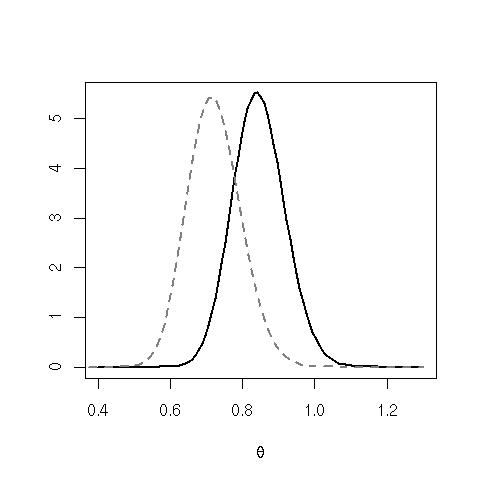
Figure 1: Representation of two gamma posterior distributions differentiating between malignant (dashes) versus non-malignant (full) breast cancer survival rates.

Then if we assume that both groups (malignant versus non-malignant) of survivors are Poisson distributed $\mathcal{P}(N_{t}\theta)$, where $N_{t}$ is the total number of patients in this age group, i.e.

$$f(x_{t}|\theta,N_{t})=e^{-\theta N_{t}}\frac{(\theta N_{t})^{x}_{t}}{x_{t}!},\quad x\in\mathbb{N}\,,$$

then we obtain a likelihood

$$L(\theta|D)=\prod_{t=1}^{3}(\theta N_{t})^{x_{t}}\exp\{-\theta N_{t}\}$$

which, under an exponential $\theta\sim\mathcal{E}xp(2)$ prior—whose rate $2$ is chosen here for illustration purposes—, leads to the posterior

$$\pi(\theta|D)\propto\theta^{x_{1}+x_{2}+x_{3}}\exp\left\{-\theta(2+N_{1}+N_{2}+N_{3})\right\}$$

i.e. a Gamma $\Gamma(x_{1}+x_{2}+x_{3}+1,2+N_{1}+N_{2}+N_{3})$ distribution. The choice of the exponential parameter corresponds to a $50\%$ survival probability. In the case of the non-malignant breast cancers, the parameters of the Gamma distribution are $a=136$ and $b=161$, while, for the malignant cancers, they are $a=96$ and $b=133$. Figure 1 shows the difference between those posteriors.

1.2 Extension to improper priors

In many situations, it is useful to extend the above setup to prior measures that are not probability distributions but $\sigma$-finite measures with infinite mass, i.e.

$$\int_{\Theta}\pi(\theta)\text{d}\nu(\theta)=+\infty,$$

since, provided that

$$\int_{\Theta}f(x|\theta)\pi(\theta)\text{d}\nu(\theta)<+\infty,$$ (3)

almost everywhere (in $x$), the quantity (2) is still well-defined as a probability density as when using a regular posterior probability as prior (Hartigan 1983, Berger 1985, Robert 2001). Such extensions are justified for a variety of reasons, ranging from topological coherence—limits of Bayesian procedures often partake of their optimality properties (Wald 1950) and should therefore be included in the range of possible procedures—to robustness—a measure with an infinite mass is much more robust than a true probability distribution with a large variance—and improper priors are typically encountered in situations where there is little or no prior information, inducing flat, i.e. uniform, distributions on the parameter space (or on some transforms of the parameter space). Indeed it is quite common, for complex models, to have little or no information on some of the parameters present in the model and using improper priors for such parameters has many advantages. Note however that in such cases the marginal density $m(x)$ does not define a probability on $\mathcal{X}$ (and that the existence condition (3) needs to be checked). This drawback has an importance consequence for Bayesian model comparison as explained in Section 5.

Note also that some improper priors never allow for well-defined posteriors, no matter how many observations there are in the sample. One such example is when the prior is $\pi(\theta)=\exp(+\theta^{2})$ and the observations are iid Cauchy. Another and less anecdotic example occurs in mixture models, under exchangeable improper priors on the components (Lee et al. 2008).

1.3 Bayesian decision theory

As a general modus vivendi, let us first stress that inference as a whole is meaningless unless it is evaluated. The evaluation of a statistical procedure, i.e. determining how well or how bad the inference performs, requires the definition of a comparison criterion, called a loss function. Set $\mathcal{D}$ the set of all possible results of the inference (corresponding to the decision set in game theory). An estimator is then a function from $\mathcal{X}$ into $\mathcal{D}$. (With an obvious abuse of notation, we will also use $\mathcal{D}$ for the set of estimators.) For instance, the aim is to estimate $\theta$, then $\mathcal{D}=\Theta$; if the aim is to test for some hypothesis, then $\mathcal{D}=\{0,1\}$, and $\mathcal{D}=\mathcal{X}_{1}$ the set of a future observation if the aim is to predict a future observation. A loss function $L$ is a function on $\Theta\times\mathcal{D}$, expressing what the loss (cost) is for considering a decision $\delta$ when $\theta$ is the true value. Typical (formal) loss functions used for estimation and test are quadratic losses ($L(\theta,\delta)=|\!|\theta-\delta|\!|^{2}$) and 0-1 losses (1 if decision is wrong, 0 if it is right), respectively. Other loss functions can (should) be constructed, depending of the problem at hand, and they are strongly related to the notion of utility function encountered in economy and game theory (Berger 1985).

Given a statistical model $(P_{\theta},\theta\in\Theta)$ on $x\in\mathcal{X}$, a prior $\pi$ on $\theta\in\Theta$ and a loss function $L)$, the (optimal) Bayesian procedure (estimator) is then defined as the decision function $\delta$ minimising the integrated risk $r(\pi,\delta)$:

$$\delta^{\pi}=\mbox{argmin}_{\delta\in\mathcal{D}}r(\pi,\delta)$$

where

$$r(\pi,\delta)=\int_{\Theta\times\mathcal{X}}L(\theta,\delta(x))f(x|\theta)\pi(\theta)\text{d}\mu(x)\text{d}\nu(\theta).$$

Such a procedure is called a Bayes estimator. Using the fact (Robert 2001), that such estimators can be computed pointwise as minimising the posterior risk: $\forall x\in\mathcal{X}$,

$$\delta^{\pi}(x) = \mbox{argmin}_{\delta\in\mathcal{D}}\int_{\Theta}L(\theta,\delta(x))\pi(\theta|x)\text{d}\nu(\theta),$$

it is possible to derive explicit expression of Bayes estimates for many common loss functions. In particular, the Bayes estimator associated with the quadratic loss and the posterior distribution $\pi(.|x)$ is the posterior mean

$$\delta^{\pi}(x)=\int_{\Theta}\theta\pi(\theta|x)\,\text{d}\theta\,.$$

Note that the integrated risk $r(\pi,\delta)$ can also be expressed as $\int_{\Theta}R(\theta,\delta)\pi(\theta)\text{d}\nu(\theta)$, where $R(\theta,\delta)=\int_{\mathcal{X}}L(\theta,\delta(x))f(x|\theta)\text{d}\mu(x)$ is the frequentist risk, so that Bayes estimates are also often optimal in the frequentist sense. (It can be shown in particular that any admissible estimator is the limit of Bayes estimators, see Berger 1985 or Robert 2001).

2 On the selection of the prior

A critical aspect is the determination of the prior distribution $\pi$ and its clear influence on the inference. It is straightforward to come up with examples where a particular choice of the prior leads to absurd decisions. Hence, for a Bayesian analysis to be sound the prior distribution needs to be well-justified. Before entering into a brief description of the various ways of constructing prior distributions, note that as part of model checking, it is necessary in every Bayesian analysis to assess the influence of the choice of the prior, for instance through a sensitivity analysis. Since the prior distribution models the knowledge (or uncertainty) prior to the observation of the data, the sparser the prior information is, the flatter the prior should be. The advantage of incorporating prior information via a prior distribution is rather universally accepted and we therefore first describe ways of eliciting prior distributions from prior knowledge.

2.1 Elicited priors

The elicitation of prior distributions from prior knowledge consists in the construction of the prior probability $\pi(\theta)$ using all items of prior information available to the modeller. This prior information may come from expert opinions or from bibliographic data or yet from earlier analyses, as in meta-analysis. There exists a vast literature on prior elicitation based on expert opinions, which is a much more complex process than is usually acknowledged in most Bayesian statistical notebooks, see Section 2 of this book for a more complete discussion on prior elicitation based on expert opinions.

In particular the prior information is rarely rich enough to entirely define a prior distribution, therefore it is customary to choose a prior distribution within a parametric class of possible distributions: $\pi(\theta|\gamma)$, where $\gamma\in\Gamma$ is called a hyperparameter. In such cases the prior information is summarised through the choice of $\gamma$. For instance, Albert et al. (2008) use bibliographic prior information to construct a prior distribution on the probability of cross-contamination from a contaminated broiler in a household, say $p$. The prior distribution of $p$ is assumed to be a Beta $\mathcal{B}e(a,b)$ distribution,

$$\pi(p|a,b)\propto p^{a-1}(1-p)^{b-1}\,,\quad 0<p<1\,,$$

and the parameters $(a,b)$ of the Beta distribution are assessed using two cross–contamination models in the literature which lead to a probability of transfer between $1/3$ and $2/3$, which was translated into a $\mbox{Beta}(8,8)$ prior on $p$, as it corresponds to a prior mean of $0.5$ and to a $95\%$ prior confidence interval equal to $(0.27,0.73)$. See also Dupuis (1995) for an example of expert elicitation of the Beta parameters on some capture and survival probabilities in a lizard population, or the Chapter of Böcker, Crimmi and Fink in this volume where beta priors are elicited to model correlations between risk types.

2.2 Conjugate priors

Among the possible parametric families $\pi(\theta|\gamma)$, $\gamma\in\Gamma$, conjugate priors form appealing parametric families, merely for computational reasons (Berger 1985, Robert 2001). A family of distribution prior distributions $\pi(\theta|\gamma)$, is said to be conjugate to the likelihood $f(x|\theta)$ if the posterior also belongs to the same family, i.e. when the prior is equal to $\pi(\theta|\gamma_{0})$ then there exists a $\gamma(x,\gamma_{0})\in\Gamma$ such that the posterior is equal to $\pi(\theta|\gamma(x,\gamma_{0}))$. The actualisation of the information due to observing the data $x$ is then modelled as a change of hyperparameter from $\gamma_{0}$ to $\gamma(x,\gamma_{0})$. Exponential families (as models for the observation $x$) are almost in one-to-one correspondence with sampling distributions allowing for conjugate priors. As an example, Carlin and Louis (2001) consider an observed random variable $X$ that is the number of pregnant women arriving at a given hospital to deliver their babies within a given month, which they model as a Poisson $\mathcal{P}(\theta)$ distribution with parameter $\theta>0$. A conjugate family of priors for the Poisson model is the collection of gamma distributions $\Gamma(a,b)$, since

$$f(x|\theta)\pi(\theta|a,b)\propto\theta^{a-1+x}e^{-(b+1)\theta}$$

leads to the posterior distribution of $\theta$ given $X=x$ being the gamma distribution $\Gamma(a+x,b+1)$. The computation of estimators, of confidence regions—called credible regions within the Bayesian literature to distinguish the fact that those regions are evaluated on the parameter space rather than on the observation space (Berger 1985)—or of other types of summaries of interest on the posterior distribution then becomes straightforward. For instance in the above Poisson–Gamma example, the Bayesian estimator of the average number of arrivals, associated with the quadratic loss, is given by $\hat{\theta}=(a+x)/(b+1)$, the posterior mean.

The apparent simplicity of conjugate priors should however not make them excessively appealing, since there is no strong justification to their use. One of the difficulties with such families of priors is the influence of the hyperparameter $\gamma_{0}$. If the prior information is not rich enough to justify a specific value of $\gamma$, fixing $\gamma=\gamma_{0}$ arbitrarily is problematic, since it does not take into account the prior uncertainty on $\gamma_{0}$ itself. To improve on this aspect of conjugate priors, a usual fix is to consider a hierarchical prior, i.e. to assume that $\gamma$ itself is random and to consider a probability distribution with density $q$ on $\gamma$, leading to

$$\theta|\gamma \sim \pi(\theta|\gamma)$$

$$\gamma \sim q(\gamma)\,,$$

as a joint prior on $\theta,\gamma)$. The above is equivalent to considering, as a prior on $\theta$

$$\pi(\theta)=\int_{\Gamma}\pi(\theta|\gamma)q(\gamma)\text{d}\gamma\,.$$

Obviously $q$ may also depend on some hyperparameters $\eta$. Higher order levels in the hierarchy are thus possible, even though the influence of the hyper(-hyper-)parameter $\eta$ on the posterior distribution of $\theta$ is usually smaller than that of $\gamma$. But multiple levels are nonetheless useful in complex populations as those found in animal breeding (Sørensen and Gianola 2002).

In many applications prior information is quite vague or at least vague enough on some parts of the model, in which case it is important to derive priors that have desirable properties and that are as little arbitrary or subjective as possible. Such constructions are commonly called non informative. While this denomination is misleading, and should be replaced by the less judgemental reference prior denomination, we nonetheless follow suit and use it in the following subsections, since it is the most common denomination found in the literature (Kass and Wasserman 1996).

2.3 Non informative priors

Non informative priors are expected to be flat distributions, possibly improper. An apparently natural way of constructing such priors would be to consider a uniform prior, however this solution has many drawbacks, the worst one being that it is not invariant under a change of parameterisation. To understand this consider the example of a Binomial model: the observation $x$ is a $\mathcal{B}(n,p)$ random variable, with $p\in(0,1)$ unknown. The uniform prior $\pi(p)=1$ could then sound like the most natural non informative choice; however, if, instead of the mean parameterisation by $p$, one considers the logistic parameterisation $\theta=\log(p/(1-p))$ then the uniform prior on $p$ is transformed into the logistic density

$$\pi(\theta)=e^{\theta}/(1+e^{\theta})^{2}$$

by the Jacobian transform, which obviously is not uniform.

To circumvent this lack of invariance per reparameterisation, Jeffreys (1939) proposed the following choice now known as Jeffreys’ prior

$$\pi(\theta) \propto \sqrt{|i(\theta)|},$$ (4)

where $i(\theta)$ is the Fisher-information matrix and $|i(\theta)|$ denotes its determinant. The above construction is obviously invariant per reparameterisation and has many other interesting features specially in one-dimensional setups (see Robert et al. 2009 for a reassessment of Jeffreys’ impact on Bayesian statistics). In particular, in the one-dimensional parameter case, the Jeffreys prior is also the matching prior (see Robert 2001, Chapters 3 and 8), and the reference prior defined by Bernardo (Bernardo 1979, Clarke and Barron 1990). For instance, when $P_{\theta}$ is a location family, i.e. when $f(x|\theta)=g(x-\theta)$, the Fisher information is constant and thus the Jeffreys prior is $\pi(\theta)=1$. Note that in many cases like the above the Jeffreys prior is improper.

In multivariate setups, Jeffreys’ construction is not so well-justified and it may lead to not-so-well-behaved priors. A famous example is the Neyman–Scott problem where two groups of observations are such that in each group all observations are distributed from $x_{i,j}\sim\mathcal{N}(\mu_{i},\sigma^{2})$, $i=1,...,n$, $j=1,2$. In this case Jeffreys’ prior is given by $\pi(\mu_{1},...,\mu_{n},\sigma)\propto\sigma^{-(n+1)}$, and the Bayes estimator of $\sigma^{2}$ associated with the quadratic loss function is equal to

$$\mathbb{E}^{\pi}\left[\sigma^{2}|x_{1,1},...,x_{n,2}\right]=\sum_{i=1}^{n}\frac{(x_{i,1}-x_{i,2})^{2}}{4(n-1)}\,,$$

which converges to $\sigma^{2}/2$ as $n$ goes to infinity, thus leading to an inconsistent estimate. Although this seems like an artificial example it is actually of wider interest, since in the normal linear regression model Jeffreys’ prior is proportional to $\sigma^{-p-2}$ where $p$ is the number of covariates. This dependence on $p$ makes it rather unappealing, even though the alternative $g$-prior of Zellner (1986) discussed below suffers from the same drawback. Another standard example discussed further in Section 4 is when estimating $||\theta||^{2}$ when $\theta$ is the $n$-dimensional mean of an $n$-dimensional normal vector.

The ultimate attempt to define a non informative prior is in our opinion Bernardo’s (1979) definition through the information theoretical device of Kullback divergence (see also Berger and Bernardo 1992 or Berger et al. 2009). The idea is to split the parameter into groups say $(\theta_{(1)},...,\theta_{(p)})$ where $\theta_{(1)}$ is more interesting than $\theta_{(2)}$, which is more interesting than $\theta_{(3)}$ and so on. This can be seen as a generalisation of the usual splitting into a parameter of interest and a nuisance parameter. Then the Bernardo’s reference prior is constructed iteratively as some sorts of Jeffreys’ priors in each of the submodels, see also Robert (2001) for a more precise description of the iterative construction. Quite obviously, this is not the unique possible approach, it depends on a choice of information measure, does not always lead to a solution, requires an ordering of the model parameters that involves some prior information (or some subjective choice) but, as long as we do not think of those reference priors as representing ignorance (Lindley 1971), they can indeed be taken as reference priors, upon which everyone could fall back when the prior information is missing (Kass and Wasserman 1996).

2.4 Some asymptotic results

A well-known phenomenon is the decrease of influence of the prior as the sample size (or the information in the data) increases. We shall recall here these results in the simpler case of i.i.d observations, however these results can be extended to non i.i.d. cases such as dependent observations under stationary and mixing properties, Gaussian processes and so on. Generally speaking in most parametric cases, the posterior distribution concentrates towards the true parameter value as $n$ goes to infinity so that posterior estimates will converge to the true values, as $n$ goes to infinity. This first type of results ensures that point estimates are satisfactory, as far as asymptotic convergence is concerned.

Another important aspect of the asymptotic analysis of Bayesian procedures is to understand how the measures of uncertainty derived from the posterior can be related to frequentist measures of uncertainty. Such a relation can be deduced from the Bernstein Von Mises property, which can be stated in the following way: Assume that the vector of observations $x=(x_{1},...,x_{n}):=x^{n}$ is made of i.i.d observations from a distribution $f(.|\theta)$, which is regular, see for instance Ghosh and Ramamoorthi (2003) for more precise conditions, and let $\pi$ be a prior density, which is positive and continuous on $\Theta$, then the posterior distribution can be approximated in the following way, when $n$ goes to infinity: for all $A\subset\Theta$

$$P^{\pi}\left[\sqrt{n}(\theta-\hat{\theta})\in A|x^{n}\right]\approx P\left[\mathcal{N}(0,i_{1}(\hat{\theta})^{-1})\in A\right],$$

where $\hat{\theta}$ is the maximum likelihood estimator and $i_{1}(\hat{\theta})$ is the Fisher information matrix per observation calculated at $\theta=\hat{\theta}$. In other words the posterior distribution resembles a Gaussian distribution centred at $\hat{\theta}$ with covariance matrix $i^{-1}(\hat{\theta})/n$, when $n$ is large.

This result has many interesting implications. The first consequence is that, to first order, the influence of the prior disappears as $n$ goes to infinity. It also allows for quick approximate computations in the case of large samples, and it implies that to first order Bayesian and frequentist inference (based on the likelihood) essentially give the same answers. Although devising procedures giving the same answers as frequentist procedures is not an ultimate aim of the Bayesian analysis, it is of importance to ensure that Bayesian procedures ultimately have also good frequentist properties. The asymptotic equivalence between the Bayesian and the frequentists answers (to first order) hold in wide generality for finite dimensional models. When the dimension of the parameter grows with the number of observations or is infinite, then this is often not true anymore, see for instance Freedman (1999) and Rivoirard and Rousseau (2009).

Although these asymptotic results have a strong frequentist flavour, in the sense that they are obtained by assuming that there is a fixed true parameter $\theta_{0}$ and as new data comes in the posterior concentrates around the true parameter like a Gaussian distribution, they are also appealing from the subjectivists points of view where probabilities represent degrees of belief and there are no objective probability model, see Diaconis and Freedman (1986) for a more precise discussion on this issue.

3 Measures of uncertainty: credible regions

Recall that the whole inference about $\theta$ is deduced from the posterior distribution, $\pi(\theta|x)$, including estimates as major summaries, but the posterior distribution gives us much more information than simply point estimates. In particular, different measures of uncertainty can be derived from the posterior and among the various measures credible regions are the most popular. A set $C\subset\Theta$ is an $\alpha$ - credible region if and only if

$$P^{\pi}\left[\theta\in C|x\right]\geq 1-\alpha.$$ (5)

Contrariwise to frequentist confidence regions, the notion of coverage probability is directly understood as a probability on $\theta$ and is therefore straightforward to interpret. Among all credible regions defined by (5), those having minimal volume are particularly interesting. It turns out, see Robert (2001), that they are defined as highest posterior density (HPD) regions:

$$C_{\alpha}^{\pi}=\{\theta;\pi(\theta)f(x|\theta)\geq k_{\alpha}(x)\}$$

where $k_{\alpha}(x)$ is the largest value such that

$$P^{\pi}\left[\theta\in C_{\alpha}^{\pi}|x\right]\geq 1-\alpha.$$

(Note that we define the bound $k_{\alpha}(x)$ in terms of the product prior$\times$likelihood in order to bypass the difficulty with the normalising constant $m(x)$.)

Although the analytic determination of $k_{\alpha}(x)$ is often challenging, the approximation of this bound based on a sample from $\pi(\theta|x)$, $\theta^{(1)},\ldots,\theta^{(p)}$, can be easily derived from an ordering of the values $\pi(\theta^{(i)})f(x|\theta^{(i)})$ as the corresponding $(1-\alpha)$-th quantile. For instance, if a Poisson $X\sim\mathcal{P}(\theta)$ count is associated with a Gamma $\Gamma(a,b)$ prior, the posterior $\Gamma(a+x,b+1)$ leads to the HPD region

$$\{\theta;\theta^{a+x-1}\,\exp(-(b+1)\theta)\geq k_{\alpha}(x)\}$$

whose determination requires a numerical construct. On the other hand, if a sample $\theta^{(1)},\ldots,\theta^{(p)}$ from the posterior $\Gamma(a+x,b+1)$ is available, then the HPD bound $k_{\alpha}(x)$ can be estimated as the $(1-\alpha)$-th quantile of the values $[\theta^{(i)}]^{a+x-1}\,\exp(-(b+1)\theta^{(i)})$’s. Figure 2 illustrates a similar derivation in the case of a normal $\mathcal{N}(\theta,\sigma^{2})$ model with both parameters unknown.

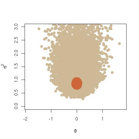
Figure 2: Representation of a Gibbs sample of $10^{3}$ values of $(\theta,\sigma^{2})$ for the normal model, $x_{1},\ldots,x_{n}\sim\mathcal{N}(\theta,\sigma^{2})$ with $\overline{x}=0$, $s^{2}=1$ and $n=10$, under Jeffreys’ prior, along with the pointwise approximation to the $10\%$ HPD region (in darker hues) (Source: Robert and Wraith 2009).

Credible regions have nice interpretations and are optimal under a volume criterion, as Bayesian estimators of the confidence sets $C$. In a wide generality, they further attain good frequentist coverage in the sense that $\mathbb{P}_{\theta}(\theta\in C)=1-\alpha+\text{O}(n^{-1/2})$ for most prior distributions $\pi$, where $n$ denotes the sample size (Welch and Peers 1963, Robert 2001, Chapter 5). Credible regions however suffer from a lack of invariance to changes of parameterisation, i.e. if $\theta$ is a given parameterisation of interest and $C_{\alpha}^{\pi}$ is the HPD region constructed as above, then if $\eta=g(\theta)$ is another parameterisation, $g(C_{\alpha}^{\pi})=\{\eta=g(\theta);\theta\in C_{\alpha}^{\pi}\}$ is not necessarily the HPD region for the $\eta$ parameterisation (see Druilhet and Marin 2007 for a detailed analysis of this phenomenon).

4 Nuisance parameters : integrated likelihood

In many applied problems, one is only interested in some components of the parameter, the remaining part of the parameter being then called the nuisance parameter. This distinction opposes the parameter of interest, say $\psi$ within $\theta=(\psi,\lambda)$, where $\psi$ is the parameter of interest and $\lambda$ is the nuisance parameter. Dealing with nuisance parameters is quite problematic in a frequentist framework, whether one is interested in parameter estimation, in confidence regions determination or in testing. Likelihood approaches need to define proper likelihoods for $\psi$, which in complete generality is not possible. Hence, they use approximations and modifications of proper likelihoods such as partial likelihoods or modified profile likelihoods, see Severini (2000) for a more complete discussion on these issues.

On the opposite, the Bayesian framework offers is a most natural way of dealing with nuisance parameters and for defining proper profile likelihoods : integrating out the nuisance parameter. In other words the Bayesian marginal likelihood for $\psi$ under the prior $\pi(\lambda|\psi)$ is given by

$$f_{\pi}(x|\psi) = \int_{\lambda}f(x|\psi,\lambda)\,\text{d}\pi(\lambda|\psi).$$ (6)

This approach offers many advantages: (1) If the conditional prior $\pi(\lambda|\psi)$ is proper, then $f_{\pi}(x|\psi)$ as defined in (6) is a proper likelihood, in the sense that it is the density of $x$ under some model parameterised by $\psi$ alone; (2) Integrating $\lambda$ out implicitly takes into account the uncertainty on $\lambda$, contrary to the profile likelihood, or to any other kind of plug-in likelihood defined by $f(x|\psi,\hat{\lambda}_{\psi})$, where $\hat{\lambda}_{\psi}$ is some estimate of $\lambda$ given $\psi$. In particular uncertainty measures derived from $f_{\pi}(x|\psi)$ are not biased downwards due to the replacement of $\lambda$ by $\hat{\lambda}_{\psi}$. Hence there is no need to correct further for this uncertainty, which is usually necessary when dealing with plug-in likelihoods, leading to penalised likelihoods. This is of particular interest in model selection, when the parameter of interest is the model itself, as discussed in Section 5.

However, if $\pi(\lambda|\psi)$ is an improper prior, then $f_{\pi}(x|\psi)$ is not necessarily a likelihood, in particular $\int_{\mathcal{X}}f_{\pi}(x|\theta)\,\text{d}x=+\infty$ may occur. A well-known example of such misbehaviour is the case of the so-called marginalisation paradoxes, see for instance Robert (2001, Chapter 3). As another example of badly behaved marginal likelihood, consider the case presented in Robert (2001, Chapter 3) and Liseo (2006) where the observations $x_{i}\sim\mathcal{N}(\mu_{i},1)$, $i=1,...,p$, are independent and where the parameter of interest is $\psi=|\!|\mu|\!|^{2}/p=\sum_{i=1}^{p}\mu_{i}^{2}/p$ where $\mu=(\mu_{1},...,\mu_{p})$ and the nuisance parameter is $\lambda=\mu/|\!|\mu|\!|$, the direction of the vector $\mu$. A natural flat prior on $\lambda$ is the uniform distribution on the $p$-dimensional sphere for $\lambda$ and the scale prior $\pi(\psi)=1/\sqrt{\psi}$, leading to a well-behaved marginal likelihood, see Berger et al. (1998b) for precise calculations. However if one considers instead the Jeffreys prior on $\mu$, i.e. $\pi(\mu)=1$, then the posterior distribution of $\psi$ is a chi-square distribution with $p$ degrees of freedom and non-centrality parameter $|\!|x|\!|^{2}$, which is not a well-behaved posterior. In particular the posterior mean of $\lambda$ is equal to $\hat{\psi}=|\!|x|\!|^{2}/p+1$ and satisfies $\hat{\psi}-\psi\rightarrow 2$ as $p$ goes to infinity.

The above examples do not imply that one should not use improper priors on nuisance parameters, since in most cases little information is known on those parameters. Rather they show that one needs to be quite careful in selecting improper priors in such cases. The construction of Bernardo’s (1979) reference priors is particularly relevant in such frameworks.

In the following section, we describe Bayesian testing and Bayesian model comparison or model selection. It is to be noted that model selection can be viewed as a specific example of nuisance parameter framework, where the parameter of interest is the model and the nuisance parameters are the parameters in each model.

5 Testing versus model comparison

5.1 Bayes factors

The most standard Bayesian answer to a testing problem for hypotheses written as $H_{0}:\,\theta\in\Theta_{0}$ for the null and as $H_{1}:\,\theta\in\Theta_{1}$ for the alternative, is the Bayesian estimate corresponding to the 0–1 loss function, i.e. to the procedure accepting $H_{0}$ if and only if

$$P^{\pi}\left[\Theta_{0}|x\right]>P^{\pi}\left[\Theta_{1}|x\right]\,.$$

In less formal terms, the null hypothesis is accepted if it is more probable under the posterior distribution than under the alternative, which is a very intuitive answer. To constrain the impact of the prior probabilities, a different quantity is usually adopted, namely the Bayes factor (Kass and Raftery 1995), which is defined by Jeffreys (1939), Jaynes (2003) as

$$B_{01}=\displaystyle{\frac{\pi(\Theta_{0}|x)}{\pi(\Theta_{1}|x)}\bigg{/}\frac{\pi(\Theta_{0})}{\pi(\Theta_{1})}}=\frac{\displaystyle{\int_{\Theta_{0}}f(x|\theta)\pi_{0}(\theta)\text{d}\theta}}{\displaystyle{\int_{\Theta_{1}}f(x|\theta)\pi_{1}(\theta)\text{d}\theta}}\,.$$

Note that the posterior odds can be recovered from the Bayes factor by assigning the appropriate prior probabilities on each of both models, contradicting the criticism of Templeton (2008) that the Bayes factor is not scaled in probability terms. Interestingly $B_{10}=1/B_{01}$, hence there is no asymmetry in the definition and construction of Bayes factor, contrariwise to the Neyman–Pearson approach. We do not believe that this is a drawback and would rather question the interest in forcing such an asymmetry in the Neyman–Pearson tests.

The Bayes factor, a monotonic transform of the posterior probability of $H_{0}$ which eliminates the influence of the prior weight $\pi(\Theta_{0})$, has a similar interpretation to the classical likelihood ratio. As noted in the previous section, by integrating out the parameters within each hypothesis, the uncertainty on each parameter is taken into account, which induces a natural penalisation for richer models, as intuited by Jeffreys (1939) (variation is random until the contrary is shown; and new parameters in laws, when they are suggested, must be tested one at a time, unless there is specific reason to the contrary). Although we strongly dislike using the term because of its undeserved weight of academic authority, the Bayes factor acts as a natural Ockham’s razor. The well-known connection with the BIC (Bayesian information criterion, see Robert 2001, Chapter 5), with a penalty term of the form $d\log n/2$, makes explicit the penalisation induced by Bayes factors in regular parametric models. However it goes beyond this class of models, and in much greater generality, the Bayes factor corresponds asymptotically to a likelihood ratio with a penalty of the form $d^{*}\log n^{*}/2$ where $d^{*}$ and $n^{*}$ can be viewed as the effective dimension of the model and the effective number of observations, respectively, see (Berger et al. 2003, Chambaz and Rousseau 2008). The Bayes factor therefore offers the major interest that it does not require to compute a complexity measure (or penalty term)—in other words, to define what is $d^{*}$ and what is $n^{*}$—, which often is quite complicated and may depend on the true distribution.

5.2 Difficulties

The inferential problems of Bayesian model selection and of Bayesian testing are clearly those for which the most vivid criticisms can be found in the literature: witness Senn (2008) who states that the Jeffreys-subjective synthesis betrays a much more dangerous confusion than the Neyman-Pearson-Fisher synthesis as regards hypothesis tests. We find this suspicion rather intriguing given that the Bayesian approach is the only one giving a proper meaning to the probability of a null hypothesis, $\mathbb{P}(H_{0}|x)$, since alternative methodologies can at best specify a probability value on the sampling space, i.e. on the wrong dual space.

If we consider the special case of point null hypotheses—which is not such limited a scope since it includes all variable selection setups—, there is a difficulty with using a standard prior modelling in this environment. As put by Jeffreys (1939), when considering whether a location parameter $\alpha$ is $0$ [when] the prior is uniform, we should have to take $f(\alpha)=0$ and $B_{10}$ would always be infinite. This is therefore a case when the inferential question implies a modification of the prior, justified by the information contained in the question. While avoiding the whole issue is a solution, as with Gelman (2008) having no patience for statistical methods that assign positive probability to point hypotheses of the $\theta=0$ type that can never actually be true, considering the null and the alternative hypotheses as two different models allows for a Bayes factor representation and corresponds to assigning a positive probability to the null hypothesis.

In our view, one of the major drawbacks of Bayes factors - or even posterior odds - is that they cannot be used under improper priors, for lack of proper normalising constants. This is even more acute a difficulty than what is described in Section 4, because the Bayes factor is simply not defined under improper priors, for any sample size. Solutions have been proposed, akin to cross-validation techniques in the classical domain (Berger and Pericchi 1996, Berger et al. 1998a), but they are somehow too ad-hoc to convince the entire community (and obviously beyond). In some situations, when parameters shared by both models have the same meaning in each of the models, an improper prior can be used on these parameters, in both models.

For instance, when considering variable selection in a regression model,

$$\mathbf{y}|\mathbf{X},\beta,\sigma\sim\mathcal{N}(\mathbf{X}\beta,\sigma^{2}I_{n})\,,$$

e.g. when deciding whether or not the null hypothesis $H_{0}:\beta_{1}=0$ holds, the relevant non informative prior distribution is Zellner’s (1986) $g$-prior, where $\pi(\beta|\sigma)$ corresponds to a normal $\mathcal{N}(0,n\sigma^{2}(\mathbf{X}^{\text{T}}\mathbf{X})^{-1})$ distribution on $\beta$ and a “marginal” improper prior on $\sigma^{2}$, $\pi(\sigma^{2})=\sigma^{-2}$. This means that, when considering the submodel corresponding to the null hypothesis $H_{0}:\beta_{1}=0$, with parameters $\beta^{(-1)}$ and $\sigma$, we can also use the “same” $g$-prior distribution

$$\beta^{(-1)}|\sigma,\mathbf{X}\sim\mathcal{N}(0,n\sigma^{2}(\mathbf{X}_{-1}^{\text{T}}\mathbf{X}_{-1})^{-1})\,,$$

where $\mathbf{X}_{-1}$ denotes the regression matrix missing the column corresponding to the first regressor, and $\sigma^{2}\sim\pi(\sigma^{2})=\sigma^{-2}$. Since $\sigma$ is a nuisance parameter in this case, we may use the improper prior on $\sigma^{2}$ as common to all submodels and thus avoid the indeterminacy in the normalising factor of the prior when computing the Bayes factor

$$B_{01}=\dfrac{\int f(\mathbf{y}|\beta_{-1},\sigma,\mathbf{X})\pi(\beta^{(-1)}|\sigma,\mathbf{X}_{1})\frac{\text{d}\beta_{-1}\,\text{d}\sigma}{\sigma^{2}}}{\int f(\mathbf{y}|\beta,\sigma,\mathbf{X})\pi(\beta|\sigma,\mathbf{X})\frac{\text{d}\beta\,\text{d}\sigma}{\sigma^{2}}}$$

Figure 3 reproduces an output from Marin and Robert (2007) that illustrates how this default prior and the corresponding Bayes factors can be used in the same spirit as significance levels in a standard regression model, each Bayes factor being associated with the test of the nullity of the corresponding regression coefficient. For instance, only the intercept and the coefficients of $X_{1},X_{2},X_{4},X_{5}$ are significant. This output mimics the standard lm R function outcome in order to show that the level of information provided by the Bayesian analysis goes beyond the classical output, not to show that we can get similar answers to those of a least square analysis since, else, if the Bayes estimator has good frequency behaviour then we might as well use the frequentist method (Wasserman 2008). (While computing issues are addressed in the following Chapter, we stress that all items in the table of Figure 3 are obtained via closed form formulae.)

	Estimate	BF	log10(BF)
(Intercept)	9.2714	26.334	1.4205 (***)
X1	-0.0037	7.0839	0.8502 (**)
X2	-0.0454	3.6850	0.5664 (**)
X3	0.0573	0.4356	-0.3609
X4	-1.0905	2.8314	0.4520 (*)
X5	0.1953	2.5157	0.4007 (*)
X6	-0.3008	0.3621	-0.4412
X7	-0.2002	0.3627	-0.4404
X8	0.1526	0.4589	-0.3383
X9	-1.0835	0.9069	-0.0424
X10	-0.3651	0.4132	-0.3838

evidence against H0: (****) decisive, (***) strong, (**) substantial, (*) poor

Figure 3: R output of a Bayesian regression analysis on a processionary caterpillar dataset with ten covariates analysed in Marin and Robert (2007). The Bayes factor on each row corresponds to the test of the nullity of the corresponding regression coefficient.

The major criticism addressed to the Bayesian approach to testing is therefore that it is not interpretable on the same scale as the Neyman-Pearson-Fisher solution, namely in terms of probability of Type I error and of power of the tests. In other words, frequentist methods have coverage guarantees; Bayesian methods don’t; 95 percent frequentist intervals will live up to their advertised coverage claims (Wasserman 2008). A natural question is then to question the appeal of such frequentist properties when considering a single dataset, i.e. in Jeffreys’ (1939) famous words, a hypothesis that may be true may be rejected because it had not predicted observable results that have not occurred, especially when considering that $p$-values may be inadmissible estimators (Hwang et al. 1992). From a decisional perspective—with which the frequentist properties should relate—, a classical Neyman-Pearson-Fisher procedure is never evaluated in terms of the consequences of rejecting the null hypothesis, even though the rejection must imply a subsequent action towards the choice of an alternative model. Therefore, complaining that having a high relative probability does not mean that a hypothesis is true or supported by the data (Templeton 2008), simply because the Bayesian approach is relative in that it posits two or more alternative hypotheses and tests their relative fits to some observed statistics (Templeton 2008), is missing the main purpose of tests, which is not to validate or invalidate a golden model per se but rather to infer a working model that allows for acceptable predictive properties.

5.3 Model choice

For model choice, i.e. when several models are under comparison for the same observation

$$\mathfrak{M}_{i}:x\sim f_{i}(x|\theta_{i})\,,\qquad i\in\mathfrak{I}\,,$$

where $\mathfrak{I}$ can be finite or infinite, the usual Bayesian answer is similar to the Bayesian tests as described above. The most coherent perspective (from our viewpoint) is actually to envision the tests of hypotheses as particular cases of model choices, rather than trying to justify the modification of the prior distribution criticised by Gelman (2008). This also also to incorporate within model choice the alternative solution of model averaging, proposed by Madigan and Raftery (1994), which strives to keep all possible models when drawing inference.

The idea behind Bayesian model choice is to construct an overall probability on the collection of models $\cup_{i\in\mathfrak{I}}\mathfrak{M}_{i}$ in the following way: the parameter is $\theta=(i,\theta_{i})$, i.e. the model index and given the model index equal to $i$, the parameter $\theta_{i}$ in model $\mathfrak{M}_{i}$, then the prior measure on the parameter $\theta$ is expressed as

$$\text{d}\pi(\theta)=\sum_{i\in\mathfrak{I}}p_{i}\text{d}\pi_{i}(\theta_{i}),\quad\sum_{i\in I_{i}}p_{i}=1\,,$$

where both the $\pi_{i}$’s and $p_{i}$’s are part of the prior modelling, hence chosen by the experimenter. (The $\pi_{i}$’s have the natural interpretation of the traditional prior under model $\mathfrak{M}_{i}$, while the $p_{i}$’s correspond to the prior assessment of the models under comparison.) As a consequence, the Bayesian model selection associated with the 0–1 loss function and the above prior is the model that maximises the posterior probability

$$\pi({\mathfrak{M}}_{i}|x)=\dfrac{\displaystyle{p_{i}\int_{\Theta_{i}}f_{i}(x|\theta_{i})\pi_{i}(\theta_{i})\text{d}\theta_{i}}}{\displaystyle{\sum_{j}p_{j}\int_{\Theta_{j}}f_{j}(x|\theta_{j})\pi_{j}(\theta_{j})\text{d}\theta_{j}}}$$

across all models. Contrary to classical pluggin likelihoods, the marginal likelihoods involved in the above ratio do compare on the same scale and do not require the models to be nested: the criticism that complicating dimensionality of test statistics is the fact that the models are often not nested, and one model may contain parameters that do not have analogues in the other models and vice versa (Templeton 2008) is not founded. As mentioned in Section 4 integrating out the parameters $\theta_{i}$ in each of the models takes into account their uncertainty thus the marginal likelihoods $\int_{\Theta_{i}}f_{i}(x|\theta_{i})\pi_{i}(\theta_{i})\text{d}\theta_{i}$ are naturally penalised likelihoods. In many setups, the Bayesian model selector as defined above is consistent, i.e. as the number of observations increases the probability of choosing the right model goes to 1.

5.4 Other issues

The computational requirements related to handling a collection of marginal likelihoods will be addressed in the following Chapter, in connection with the review of classical solutions in Robert and Marin (2010). Interestingly enough, the most accurate approximation technique for marginal likelihoods is, when applicable, directly derived from Bayes theorem, via Chib’s (1995) rendering:

$$m(x)=\dfrac{\pi(\theta)f(x|\theta)}{\pi(\theta|x)}\approx\dfrac{\pi(\theta)f(x|\theta)}{\hat{\pi}(\theta|x)}\,,$$

where $\hat{\pi}(\theta|x)$ is a simulation-based approximation to the posterior density based on simulated latent variables. Marin and Robert (2008) illustrate this method in the setting of mixtures and Robert and Marin (2010) in the alternative case of a probit model, respectively, both of which demonstrate the precision of this approximation.

Posterior odds and Bayes factors are the most common Bayesian approaches to testing, however they are not the only ones. In particular the choice of the 0–1 loss function is not necessarily relevant or the most relevant. In some situations it might be more interesting to penalise the loss with the distance to the null hypothesis for instance, see Robert and Rousseau (2002), Rousseau (2007) where such ideas are applied to goodness of fit tests or Bernardo (2009).

6 On pervasive computing

Bayesian analysis has long been derided for providing optimal answers that could not be computed. With the advent of early Monte Carlo methods, of personal computers, and, more recently, of more powerful Monte Carlo methods (Hitchcock 2003), the pendulum appears to have switched to the other extreme and Bayesian methods seem to quickly move to elaborate computation (Gelman 2008), a feature that does not make them less suspicious: a simulation method of inference hides unrealistic assumptions (Templeton 2008). The simulation techniques that have done so much to promote Bayesian analysis in the past decades are detailed in the next Chapter and thus not described here. We nonetheless want to point out that, while simulation methods can be misused—as about any other methodology—and while Bayesian simulation seems stuck in an infinite regress of inferential uncertainty (Gelman 2008), there exist enough convergence assessment techniques (Robert and Casella 2009) to ensure a reasonable confidence about the approximation provided by those simulation methods. Thus, as rightly stressed by Bernardo (2008), the discussion of computational issues should not be allowed to obscure the need for further analysis of inferential questions.

The field of Bayesian computing is therefore very much alive and, while its diversity can be construed as a drawback by some, we do see the emergence of new computing methods adapted to specific applications as most promising, because it bears witness to the growing involvement of new communities of researchers in Bayesian advances.

References

- Albert et al. (2008) Albert, I., Grenier, E., Denis, J. and Rousseau, J. (2008). Quantitative risk assessement from farm to fork and beyond: a global Bayesian approach concerning food-borne diseases. Risk Analysis, 28:2 558–571.
- Berger (1985) Berger, J. (1985). Statistical Decision Theory and Bayesian Analysis. 2nd ed. Springer-Verlag, New York.
- Berger and Bernardo (1992) Berger, J. and Bernardo, J. (1992). On the development of the reference prior method. In Bayesian Statistics 4 (J. Berger, J. Bernardo, A. Dawid and A. Smith, eds.). Oxford University Press, London, 35–49.
- Berger et al. (2009) Berger, J., Bernardo, J. and Sun, D. (2009). Natural induction: an objective Bayesian approach. Rev. R. Acad. Cien. Serie A. Mat., 103 125–135.
- Berger et al. (2003) Berger, J., Ghosh, J. and Mukhopadhyay, N. (2003). Approximations to the Bayes factor in model selection problems and consistency issues. J. Statist. Plann. Inference, 112 241–258.
- Berger and Pericchi (1996) Berger, J. and Pericchi, L. (1996). The intrinsic Bayes factor for model selection and prediction. J. American Statist. Assoc., 91 109–122.
- Berger et al. (1998a) Berger, J., Pericchi, L. and Varshavsky, J. (1998a). Bayes factors and marginal distributions in invariant situations. Sankhya A, 60 307–321.
- Berger et al. (1998b) Berger, J., Philippe, A. and Robert, C. (1998b). Estimation of quadratic functions: reference priors for non-centrality parameters. Statistica Sinica, 8 359–375.
- Berkhof et al. (2003) Berkhof, J., van Mechelen, I. and Gelman, A. (2003). A Bayesian approach to the selection and testing of mixture models. Statistica Sinica, 13 423–442.
- Bernardo (1979) Bernardo, J. (1979). Reference posterior distributions for Bayesian inference (with discussion). J. Royal Statist. Society Series B, 41 113–147.
- Bernardo (2008) Bernardo, J. (2008). Comment on an article by Gelman. Bayesian Analysis, 3(3) 451–454.
- Bernardo (2009) Bernardo, J. (2009). Modern Bayesian inference: Foundations and objective methods. In Philosophy of Statistics (P. Bandyopadhyay and M. Forster, eds.). Amsterdam: Elsevier. (To appear).
- Bishop et al. (1975) Bishop, Y. M. M., Fienberg, S. E. and Holland, P. W. (1975). Discrete Multivariate Analysis: Theory and Practice. MIT Press, Cambridge, MA.
- Carlin and Louis (2001) Carlin, B. and Louis, T. (2001). Bayes and Empirical Bayes Methods for Data Analysis. 2nd ed. Chapman and Hall, New York.
- Chambaz and Rousseau (2008) Chambaz, A. and Rousseau, J. (2008). Bounds for Bayesian order identification with application to mixtures. Ann. Statist., 36 938–962.
- Chib (1995) Chib, S. (1995). Marginal likelihood from the Gibbs output. J. American Statist. Assoc., 90 1313–1321.
- Clarke and Barron (1990) Clarke, B. and Barron, A. (1990). Information-theoretic asymptotics of Bayes methods. IEEE Trans. Information Theory, 36 453–471.
- Diaconis and Freedman (1986) Diaconis, P. and Freedman, D. (1986). On the consistency of Bayes estimates. Ann. Statist., 14 1–26.
- Druilhet and Marin (2007) Druilhet, P. and Marin, J.-M. (2007). Invariant hpd credible sets and map estimators. Bayesian Analysis, 2(4) 681–692.
- Dupuis (1995) Dupuis, J. (1995). Bayesian estimation of movement probabilities in open populations using hidden Markov chains. Biometrika, 82 761–772.
- Freedman (1999) Freedman, D. (1999). On the Bernstein Von Mises theorem with infinite dimensional parameter. Ann. Statist., 27 1119–1140.
- Frühwirth-Schnatter (2004) Frühwirth-Schnatter, S. (2004). Estimating marginal likelihoods for mixture and Markov switching models using bridge sampling techniques. The Econometrics Journal, 7 143–167.
- Gelman (2008) Gelman, A. (2008). Objections to Bayesian statistics. Bayesian Analysis, 3(3) 445–450.
- Ghosh and Ramamoorthi (2003) Ghosh, J. and Ramamoorthi, R. (2003). Bayesian non parametrics. Springer-Verlag, New York.
- Hartigan (1983) Hartigan, J. A. (1983). Bayes Theory. Springer-Verlag, New York, New York.
- Hitchcock (2003) Hitchcock, D. H. (2003). A history of the Metropolis–Hastings algorithm. The American Statistician, 57.
- Hwang et al. (1992) Hwang, J., Casella, G., Robert, C., Wells, M. and Farrel, R. (1992). Estimation of accuracy in testing. Ann. Statist., 20 490–509.
- Jaynes (2003) Jaynes, E. (2003). Probability Theory. Cambridge University Press, Cambridge.
- Jeffreys (1939) Jeffreys, H. (1939). Theory of Probability. 1st ed. The Clarendon Press, Oxford.
- Kass and Raftery (1995) Kass, R. and Raftery, A. (1995). Bayes factors. J. American Statist. Assoc., 90 773–795.
- Kass and Wasserman (1996) Kass, R. and Wasserman, L. (1996). Formal rules of selecting prior distributions: a review and annotated bibliography. J. American Statist. Assoc., 91 343–1370.
- Lee et al. (2008) Lee, K., Marin, J.-M., Mengersen, K. and Robert, C. (2008). Bayesian inference on mixtures of distributions. In Platinum Jubilee of the Indian Statistical Institute (N. N. Sastry, ed.). Indian Statistical Institute, Bangalore.
- Lindley (1971) Lindley, D. (1971). Bayesian Statistics, A Review. SIAM, Philadelphia.
- Liseo (2006) Liseo, B. (2006). The elimination of nuisance parameters. In Handbook of Statistics (D. Dey and C. Rao, eds.), vol. 25, chap. 7. Elsevier-Sciences.
- MacKay (2002) MacKay, D. J. C. (2002). Information Theory, Inference & Learning Algorithms. Cambridge University Press, Cambridge, UK.
- Madigan and Raftery (1994) Madigan, D. and Raftery, A. (1994). Model selection and accounting for model uncertainty in graphical models using Occam’s window. J. American Statist. Assoc., 89 1535–1546.
- Marin and Robert (2007) Marin, J.-M. and Robert, C. (2007). Bayesian Core. Springer-Verlag, New York.
- Marin and Robert (2008) Marin, J.-M. and Robert, C. (2008). Approximating the marginal likelihood in mixture models. Bulletin of the Indian Chapter of ISBA, V(1) 2–7.
- Popper and Miller (1983) Popper, K. and Miller, D. (1983). The impossibility of inductive probability. Nature, 310 434.
- Rivoirard and Rousseau (2009) Rivoirard, V. and Rousseau, J. (2009). On the Bernstein Von Mises theorem for linear functionals of the density. Tech. rep., CEREMADE, Université Paris Dauphine. 0908.4167.
- Robert (2001) Robert, C. (2001). The Bayesian Choice. 2nd ed. Springer-Verlag, New York.
- Robert (2010) Robert, C. (2010). On the relevance of the Bayesian approach to Statistics. The Review of Economic Analysis, arXiv:0909.5365. (To appear.).
- Robert and Casella (2009) Robert, C. and Casella, G. (2009). Introducing Monte Carlo Methods with R. Springer-Verlag, New York.
- Robert et al. (2009) Robert, C., Chopin, N. and Rousseau, J. (2009). Theory of Probability revisited (with discussion). Statist. Science. (to appear).
- Robert and Marin (2010) Robert, C. and Marin, J.-M. (2010). Importance sampling methods for Bayesian discrimination between embedded models. In Frontiers of Statistical Decision Making and Bayesian Analysis (M.-H. Chen, D. K. Dey, P. Mueller, D. Sun and K. Ye, eds.). (To appear.).
- Robert and Rousseau (2002) Robert, C. and Rousseau, J. (2002). A mixture approach to Bayesian goodness of fit. Tech. rep., Cahiers du CEREMADE, Université Paris Dauphine.
- Robert and Wraith (2009) Robert, C. and Wraith, D. (2009). Computational methods for Bayesian model choice. In MaxEnt 2009 proceedings (A. I. of Physics, ed.). (To appear.).
- Rousseau (2007) Rousseau, J. (2007). Approximating interval hypotheses: p-values and Bayes factors. In Bayesian Statistics 8: Proceedings of the Eigth International Meeting (J. M. Bernardo, J. O. Berger, A. P. Dawid and A. F. M. Smith, eds.). Oxford University Press.
- Senn (2008) Senn, S. (2008). Comment on an article by Gelman. Bayesian Analysis, 3(3) 459–462.
- Severini (2000) Severini, T. (2000). Likelihood Methods in Statistics. Oxford University Press, Oxford.
- Sørensen and Gianola (2002) Sørensen, D. and Gianola, D. (2002). Likelihood, Bayesian, and MCMC Methods in Qualitative Genetics. Springer-Verlag, New York.
- Templeton (2008) Templeton, A. (2008). Statistical hypothesis testing in intraspecific phylogeography: nested clade phylogeographical analysis vs. approximate Bayesian computation. Molecular Ecology, 18(2) 319–331.
- Wald (1950) Wald, A. (1950). Statistical Decision Functions. John Wiley, New York.
- Wasserman (2008) Wasserman, L. (2008). Comment on an article by Gelman. Bayesian Analysis, 3(3) 463–466.
- Welch and Peers (1963) Welch, B. and Peers, H. (1963). On formulae for confidence points based on integrals of weighted likelihoods. J. Royal Statist. Society Series B, 25 318–329.
- Zellner (1986) Zellner, A. (1986). On assessing prior Distributions and Bayesian regression analysis with -prior distribution regression using Bayesian variable selection. In Bayesian inference and decision techniques: Essays in Honor of Bruno de Finetti. North-Holland / Elsevier, 233–243.