Applications of the Tunneling Method to Particle Decay and Radiation from Naked Singularities

Abstract

Following recent literature on dS instability in presence of interactions, we study the decay of massive particles in general FRW models and the emission from naked singularities either associated with $4D$ charged black holes or $2D$ shock waves, by means of the Hamilton–Jacobi tunneling method. It is shown that the two-dimensional semi-classical tunneling amplitude from a naked singularity computed in that way is the same as the one-loop result of quantum field theory.

^(a) Dipartimento di Fisica, Università di Trento
and Istituto Nazionale di Fisica Nucleare - Gruppo Collegato di Trento
Via Sommarive 14, 38123 Povo, Italia

PACS numbers:    04.62.+v, 04.20.Dw, 04.70.Dy

1 Introduction

It is well known that de Sitter (dS) space has gained tremendous importance since the discovery by Riess and Perlmutter [1, 2] that the Universe is – against any previous belief based on Einstein gravity with vanishing cosmological constant – in a current accelerating state.

As far as this fundamental issue is concerned, two very interesting papers on de Sitter space and the vacuum energy, one by A. Polyakov [3] and one by G. Volovik [4] have recently appeared. We recall that from a classical point of view, it is generally believed that dS space is stable since: (i) it has a big isometry group, namely $SO(1,4)$; (ii) linearized fluctuations of the metric do not grow exponentially with time so that they are not able to change the background dS metric; (iii) particles in dS space are excitations over a dS invariant vacuum state (cfr. [5]).
Many authors have argued [6, 7, 8, 9, 4] that these observations are not sufficient to prove the classical stability of dS space-time. In fact, whenever an interacting field theory is present, dS space is unstable because of the non-vanishing probability amplitude of massive particles radiating other massive particles. It is worth stressing that the only force acting on the particles is due to the gravitational background induced by $\Lambda$. Even if such radiating process is small for small $\Lambda$ (as it is at present time), no eternal dS space seems physically meaningful. Indeed, it is expected that the particle production will eventually stop at the point when back-reaction becomes significant. Even if it seems hard to make precise predictions about what will occur at that point, Polyakov [3] has suggested that back-reaction will finally cancel any trace of the Cosmological Constant and of dS space-time as well. The extension of (some of) these results to general FRW models should give hope that the deep analysis of Polyakov could be so extended.
The decay of composite particles in dS space-time has been investigated in [4] by means of semi-classical methods applied to a single particle path. Very remarkably, the result obtained in this way turns out to be in agreement with the asymptotic of an exact full QFT calculation given in [9]. The advantage of using the WKB approximation in favour of exact QFT machinery is evident, since the extremely complicated computations involved in [9].

In this paper, first we would like to show that Volovik’s result [4] can be extended to a general FRW space-time, making use of the so-called Hamilton–Jacobi method [10, 11, 12], implemented by using the Kodama–Hayward invariant formalism [13, 14], which can be applied to spherically symmetric space-times no matter if static or dynamical.
Here the decay of the horizon corresponds to the existence of a simple pole in the radial derivative of the action while the particle’s decay will correspond to a branch point singularity in the radial particle’s momentum. Similar results will be obtained for static black holes possessing time-like, or naked, singularities (a general reference for the study of these objects is in Harada et al [17] and references therein). They might even be produced in colliders in certain brane world models [18].
Then we apply the null expansion method within the Hamilton–Jacobi equation to see whether in a dynamical space-time region bounded by a naked singularity there is radiation which can be interpreted as coming out from it. The decay of the singularity, that if charged is eventually due to a screening by oppositely charged particles, or else its explosion [19], is again associated with a simple pole whose residue depends on which null direction one is integrating the action’s differential. As we will see, this corresponds to the different components of the radiation’s quantum stress tensor. The fact that the Reissner-Nordström static singularity does not radiate (neutral particles) illustrates how care has to be given when extrapolating two-dimensional results to four-dimensional ones.

The paper is organized in the following way: in §2 we briefly resume the Kodama–Hayward approach to spherically symmetric space-times; in §3 we apply the Hamilton–Jacobi method of tunneling to FRW space-times; §4 is devoted to the discussion of static spherically symmetric black-holes endowed with time-like singularities; in §5 we analyze the radiation from the singularity itself in a model of two-dimensional dilaton gravity. Some conclusions will follow.

2 The Kodama–Hayward formalism

We recall that in previous papers [15, 16] we considered the quantum instability of dynamical black holes using a variant of the tunneling method introduced by Parikh and Wilczek in the static case to uncover aspects of back-reaction effects [20]. These approaches are based on WKB relativistic method (see, for example [21] and more recently [22]) and only the leading terms of the production rate probability are taken into account, leaving untouched the pre-factor evaluation. Such evaluation, and possible back-reaction effects, however, are not included in the present discussion which is focused indeed, only on the leading WKB contribution to the production rate. With regard to the pre-factor issue, we limit ourselves to mention Volovik’s arguments according to which the pre-factor is likely to vanish in the case of horizon tunneling in dS space-time [23].
In our generalization of Volovik’s calculation, the use of invariant quantities plays a crucial role [15, 16]. In order to illustrate them, let us recall that any spherically symmetric metric can locally be expressed in the form

$$ds^{2}=\gamma_{ij}(x^{i})dx^{i}dx^{j}+R^{2}(x^{i})d\Omega^{2}\,,\qquad i,j\in\{0,1\}\;,$$ (2.1)

where the two-dimensional metric

$$d\gamma^{2}=\gamma_{ij}(x^{i})dx^{i}dx^{j}$$ (2.2)

is referred to as the normal metric, $\{x^{i}\}$ are associated coordinates and $R(x^{i})$ is the areal radius, considered as a scalar field in the two-dimensional normal space. We recall that to have a truly dynamical solution, i.e. to avoid Birkhoff’s theorem, the space-time must be filled with matter everywhere. Examples are the Vaidya solution, which contains a flux of radiation at infinity, and FRW solutions which contain a perfect fluid.
A relevant scalar quantity in the reduced normal space is

$$\chi(x)=\gamma^{ij}(x)\partial_{i}R(x)\partial_{j}R(x)\,,$$ (2.3)

since the dynamical trapping horizon, if it exists, is located in correspondence of

$$\chi(x)\Big{|}_{H}=0\,,$$ (2.4)

provided that $\partial_{i}\chi|_{H}\neq 0$. The Misner–Sharp gravitational energy, in units $G=1$, is defined by

$$E_{MS}(x)=\frac{1}{2}R(x)\left[1-\chi(x)\right]\,.$$ (2.5)

This is an invariant quantity on the normal space. Note also that, on the horizon, $E_{MS}|_{H}=\frac{1}{2}R_{H}$. Furthermore, one can introduce a dynamic surface gravity [15] associated with this dynamical horizon, given by the normal-space scalar

$$\kappa_{H}=\frac{1}{2}\Box_{\gamma}R\Big{|}_{H}\,.$$ (2.6)

Recall that, in the spherical symmetric dynamical case, it is possible to introduce the Kodama vector field $K$, with $(K^{\alpha}G_{\alpha\beta})^{;\beta}=0$ that can be taken as its defining property. Given the metric (2.1), the Kodama vector components are

$$K^{i}(x)=\frac{1}{\sqrt{-\gamma}}\,\varepsilon^{ij}\partial_{j}R\,,\qquad K^{\theta}=0=K^{\varphi}\;.$$ (2.7)

The Kodama vector gives a preferred flow of time and in this sense it generalizes the flow of time given by the Killing vector in the static case. As a consequence, we may introduce the invariant energy associated with a particle of mass $m$ by means of the scalar quantity on the normal space

$$\omega=-K^{i}\partial_{i}I\,,$$ (2.8)

where $I$ is the particle action which we assume to satisfy the reduced Hamilton–Jacobi equation

$$\gamma^{ij}\partial_{i}I\partial_{j}I+m^{2}=0\,.$$ (2.9)

We shall call (2.8) the Kodama, or generalized Killing energy. As we allow for non-minimal gravitational coupling, the substitution $m^{2}\rightarrow m^{2}+\xi\mathcal{R}$ is in order whenever $\xi\neq 0$, $\mathcal{R}$ being the Ricci curvature scalar and $\xi$ a dimensionless coupling constant.

3 The FRW Space-time

As a first application of the formalism, let us consider a generic FRW space-time with constant curvature spatial sections. Its line element can be written as

$$ds^{2}=-dt^{2}+a^{2}(t)\frac{dr^{2}}{1-\hat{k}r^{2}}+[a(t)r]^{2}d\Omega^{2}\;.$$ (3.1)

Here $\hat{k}:=\frac{k}{l^{2}}$, where $l$ is such that $a(t)l$ is the curvature radius of the constant curvature spatial sections at time $t$ and, as usual, $k=0,-1,+1$ labels flat, open and closed three–geometries, respectively. In this gauge, the normal reduced metric is diagonal and

$$\chi(t,r)=1-[a(t)r]^{2}\left[H^{2}(t)+\frac{\hat{k}}{a^{2}(t)}\right]\,.$$ (3.2)

The dynamical horizon is implicitly given by $\chi_{H}=0$, namely

$$R_{H}:=a(t)r_{H}=\frac{1}{\sqrt{H^{2}(t)+\frac{\hat{k}}{a^{2}(t)}}}\,,\qquad\mbox{with}\qquad H(t)=\frac{\dot{a}(t)}{a(t)}\;,$$ (3.3)

provided the space-time energy density $\rho(t)$ is positive. The surface $R_{H}(t)$ coincides with the Hubble radius as defined by astronomers for vanishing curvature, but we shall call it ’Hubble radius’ in any case. The dynamical surface gravity is given by equation (2.6) and reads

$$\kappa_{H}=-\left(H^{2}(t)+\frac{1}{2}\dot{H}(t)+\frac{\hat{k}}{2a^{2}(t)}\right)\,R_{H}(t)<0\,,$$ (3.4)

and the minus sign refers to the fact the Hubble horizon is, in Hayward’s terminology, of the inner type. According to (2.7), the Kodama vector is

$$K=\sqrt{1-\hat{k}r^{2}}(\partial_{t}-rH(t)\partial_{r})$$ (3.5)

so that the invariant Kodama energy of a particle is equal to

$$\omega=\sqrt{1-\hat{k}r^{2}}(-\partial_{t}I+rH(t)\partial_{r}I)\equiv\sqrt{1-\hat{k}r^{2}}\,\tilde{\omega}$$ (3.6)

Notice that $K$ is space-like for $ra>(H^{2}+\hat{k}/a^{2})^{-1/2}$, i.e. beyond the horizon. It follows that we can only ask for particles to be emitted in the inner region, $r<r_{H}$.
The next ingredient is the reduced Hamilton–Jacobi equation for a relativistic particle with mass parameter $m$,

$$-(\partial_{t}I)^{2}+\frac{(1-\hat{k}r^{2})}{a^{2}(t)}\,(\partial_{r}I)^{2}+m^{2}=0\,.$$ (3.7)

Making use of (3.6), one can solve for $\partial_{r}I$, namely

$$\partial_{r}I=-\frac{aH\tilde{\omega}(ar)\pm a\sqrt{\omega^{2}-m^{2}+m^{2}\,\left(H^{2}+\frac{\hat{k}}{a^{2}}\right)\,(ar)^{2}}}{1-\left(H^{2}+\frac{\hat{k}}{a^{2}}\right)\,(ar)^{2}}\,,$$ (3.8)

with the signs chosen according to which direction we think the particle is propagating. The effective mass here defines two important and complementary energy scales: if one is interested in the horizon tunneling then only the pole matters (since the denominator vanishes), and we may neglect to all the extents the mass parameter setting $m=0$ (since its coefficient vanishes on the horizon).
On the opposite, in investigating other effects in the bulk away from the horizon, such as the decay rate of composite particles, the role of the effective mass becomes relevant as the energy of the particle can be smaller than the energy scale settled by $m$, and the square root can possibly acquire a branch cut singularity.

3.1 Horizon tunneling

As an application of the last formula we may derive, following [16], the cosmic horizon tunneling rate. To this aim, as we have anticipated, the energy scale is such that near the horizon, we may neglect the particle’s mass, and note that radially moving massless particles follow a null direction. Then, along a null radial direction from the horizon to the inner region, we have

$$\delta t=-\frac{a(t)}{\sqrt{1-\hat{k}r^{2}}}\delta r.$$ (3.9)

The outgoing particle action, that is the action for particles coming out of the horizon towards the inner region, is then

$$I = \int dt\,\partial_{t}I+\int dr\,\partial_{r}I$$ (3.10)

$$= 2\int dr\partial_{r}I\,$$ (3.11)

upon solving the Hamilton–Jacobi equation (3.7) with zero mass and using (3.9). For $\partial_{r}I$ we use now Eq. (3.8), which exhibits a pole at the vanishing of the function $F(r,t):=1-(a^{2}H^{2}+\hat{k})r^{2}$, defining the horizon position. Expanding $F(r,t)$ again along a null direction, one gets

$$F(r,t)\approx+4\kappa_{H}a(t)(r-r_{H})+\dots\;,$$ (3.12)

where $\kappa_{H}$ given in (3.4) represents the dynamical surface gravity associated with the horizon.
In order to deal with the simple pole in the integrand, we implement Feynman’s $i\epsilon$ – prescription. In the final result, beside a real (irrelevant) contribution, we obtain the following imaginary part [16]

$$\Im\,I=-\frac{\pi\omega_{H}}{\kappa_{H}}\,.$$ (3.13)

This imaginary part is usually interpreted as arising because of a non-vanishing tunneling probability rate of (massless) particles across the cosmological horizon,

$$\Gamma\sim\exp\left(-2\Im\,I\right)\sim e^{-\frac{2\pi}{(-\kappa_{H})}\cdot\omega_{H}}.$$ (3.14)

Notice that, since $\kappa_{H}<0$ and $\omega_{H}>0$ for physical particles, (3.13) is positive definite. As showed in [16], this result is invariant since the quantities appearing in the imaginary part are manifestly invariant. As a consequence, we may interpret $T=-\kappa_{H}/2\pi$ as the dynamical temperature associated with FRW space-times. In particular, this gives naturally a positive temperature for de Sitter space-time, a long debated question years ago, usually resolved by changing the sign of the horizon’s energy. It should be noted that in literature, the dynamical temperature is usually given in the form $T=\frac{H}{2\pi}$ (exceptions are the papers [24]). Of course this is the expected result for dS space in inflationary coordinates, but it ceases to be correct in any other coordinate system. In this regard, the $\dot{H}$ and $\hat{k}$ terms are crucial in order to get an invariant temperature.
The horizon’s temperature and the ensuing heating of matter was foreseen several years ago in the interesting paper [25].

3.2 Decay rate of unstable particles

We are now ready to present the generalization of the result presented in [4] for de Sitter space to a generic FRW space-time. Let us consider the decay rate of composite particles in a regime where the energy of the decay product is lower than their proper mass $m$. A crucial point is to identify the energy of the particle before the decay with its Kodama energy. After the decay process, we denote by $m$ the effective mass parameter of one of the decay products (recall it may contain a curvature term). The relevant contribution to the action comes from the radial momentum given by equation (3.8). If we introduce the instantaneous radius $r_{0}$ by

$$[a(t)r_{0}]^{2}=R_{0}^{2}:=\left(1-\frac{\omega^{2}}{m^{2}}\right)R_{H}^{2}\;,$$ (3.15)

where $R_{H}$ is the horizon radius given by Eq. (3.3), then the classical forbidden region is $0<r<r_{0}$. Thus, from (3.8), we see that for the unstable particle, say with mass $m_{0}$, sitting at rest at the origin of the comoving coordinates, one has an imaginary part of the action as soon as the decay product is tunneling into this region to escape beyond $r_{0}$,

$$\Im\,I=mR_{H}\int_{0}^{R_{0}}dR\frac{\sqrt{R_{0}^{2}-R^{2}}}{R_{H}^{2}-R^{2}}\,.$$ (3.16)

The integral can be computed exactly at fixed $t$, and is

$$\Im\,I=\frac{\pi}{2}\,R_{H}\,(m-\omega)>0\,,$$ (3.17)

leading to a rate which, assuming a two-particle decay, takes the form

$$\Gamma=\Gamma_{0}e^{-2\pi\,R_{H}\,(m-\omega)}\,,$$ (3.18)

where $\Gamma_{0}$ is an unknown pre-factor depending on the coupling constant of the interaction which is causing the decay (for instance, for a $\lambda\phi^{3}$ interaction one should have $\Gamma_{0}\sim\lambda^{2}$.) Of course, each newly produced particle will itself decay, leading possibly to the instability mechanism first discussed by Myhrvold [6] in dS space.
Since the tunneling process locally conserves energy one should put $\omega=m_{0}/2$, so that the tunnelled particle will emerge in the classical region at $r=r_{0}$ with vanishing momentum. Furthermore, the result is again invariant against coordinate changes, since both $\omega$ and $R_{H}$ are invariantly defined quantities.
A particularly interesting case is the de Sitter space-time. The line element in the static patch reads

$$ds^{2}=-(1-H_{0}^{2}r^{2})dt^{2}+\frac{dr^{2}}{(1-H_{0}^{2}r^{2})}+r^{2}d\Omega^{2}\,,$$ (3.19)

in the inflationary flat patch is

$$ds^{2}=-dt^{2}+e^{2H_{0}t}d\,\overrightarrow{x}^{2}\,,$$ (3.20)

while in global coordinates

$$ds^{2}=-dt^{2}+\cosh^{2}(H_{0}t)d\Omega_{3}^{2}\,.$$ (3.21)

The so-called “fluid” static form discussed by Volovik is instead

$$ds^{2}=-dt^{2}+(dR-H_{0}Rdt)^{2}+R^{2}d\Omega^{2}\,.$$ (3.22)

As already stated, a direct calculation leads always to $\kappa_{H}=-H_{0}$ for the surface gravity and

$$\Im\,I=\frac{\pi}{2H_{0}}(m-\omega)$$ (3.23)

for the imaginary part (3.18), independently by the coordinate system in use. In the “fluid” gauge (3.22), putting $\omega=\frac{m_{0}}{2}$, the above result has been obtained by Volovik [4], in agreement with the exact result of [9].

4 Black hole’s singularities

One may investigate if the method can be extended to the case of static black holes. With regard to this, we consider the exterior region of a spherically symmetric static black hole space-time and repeat the same argument. Quite generally, we can write the line element as

$$ds^{2}=-e^{2\psi(r)}C(r)dt^{2}+C^{-1}(r)dr^{2}+r^{2}d\Omega^{2}.$$ (4.1)

The radial momentum turns out to be,

$$\int dr\,\partial_{r}I=\int dr\,\frac{\sqrt{\omega^{2}-m^{2}C(r)e^{2\psi(r)}}}{C(r)e^{\psi(r)}}\;.$$ (4.2)

The analysis of this integral is made easier by setting $\omega=0$, which should correspond to particle creation: in fact, according to the interpretation of the Kodama energy we gave before, this approximation simulates the vacuum condition. Then

$$\int dr\,\partial_{r}I=m\int_{r_{1}}^{r_{2}}dr\frac{1}{\sqrt{-C(r)}}\,,$$ (4.3)

where the integration is performed in every interval $(r_{1},r_{2})$ in which $C(r)>0$. Equation (4.3) shows that, under very general conditions, in static black hole space-times there could be a decay rate whenever a region where $C(r)$ is positive exists.

As a first example, let us analyze the Schwarzschild black hole. For the exterior (static) solution, one has $C(r)=1-2M/r>0$ and $\psi(r)=0$, thus the imaginary part diverges since the integral has an infinite range. We conclude that the space-like singularity does not emit particles. In the interior, it is possible to show that the Kodama vector is space-like, thus no energy can be introduced. A similar conclusion has been obtained also for the Big Bang cosmic singularity, the only scale factor leading to particle emission being $a(t)\sim t^{-1}$. This is like a big rip in the past.

The situation is different when a naked singularity is present. Consider a neutral particle in the Reissner–Nordström solution with mass $M$ and charge $Q>0$ (for definiteness) given by the (spherically symmetric) line element

$$ds^{2}=-\frac{(r-r_{-})(r-r_{+})}{r^{2}}dt^{2}+\frac{r^{2}}{(r-r_{-})(r-r_{+})}\,dr^{2}+r^{2}d\Omega^{2}\,.$$ (4.4)

Here $r_{\pm}=M\pm\sqrt{M^{2}-Q^{2}}$ are the horizon radii connected to the black hole mass and charge by the relations

$$M=\frac{r_{+}+r_{-}}{2},\quad Q=\sqrt{r_{+}r_{-}}\,.$$ (4.5)

The Kodama energy coincides with the usual Killing energy and

$$C(r)=\frac{(r-r_{-})(r-r_{+})}{r^{2}}\;,\qquad\mbox{and}\qquad\psi(r)=0\;.$$ (4.6)

The metric function $C(r)$ is negative in between the two horizons, so there the action is real. On the other hand it is positive within the outer communication domain, $r>r_{+}$, but also within the region contained by the inner Cauchy horizon, that is $0<r<r_{-}$. Thus, because of (4.3) and assuming the particles come created in pairs, we obtain

$$\Im\,I=-m\int_{0}^{r_{-}}\frac{r}{\sqrt{(r_{-}-r)(r_{+}-r)}}\;dr=mQ-\frac{mM}{2}\ln\left(\frac{M+Q}{M-Q}\right)\;.$$ (4.7)

Modulo the pre-factor over which we have nothing to say , there is a probability

$$\Gamma\sim\exp(-2\Im I)=\left(\frac{M-Q}{M+Q}\right)^{mM}e^{-2Qm}\;.$$ (4.8)

Pleasantly, (4.8) vanishes in the extremal limit $M=Q$. Being computed for particles with zero energy, we can interpret this as a particle creation effect by the strong gravitational field near the singularity. Since the electric field is of order $Q/r^{2}$ near $r=0$, there should also be a strong Schwinger’s effect. In that case one should write the Hamilton–Jacobi equation for charged particles. It would be an interesting question whether this effect could lead to a screening of the singularity, and ultimately to its disappearance.

Next we consider the hairy black hole solution in the Jordan frame, for $\Lambda=\frac{3}{\ell^{2}}>0$. This is a black hole solution in the Einstein theory with a self-interacting and conformally coupled scalar field (see[26, 27]). One has

$$C(r)=-\frac{r^{2}}{\ell^{2}}+\frac{(r+r_{0})^{2}}{r^{2}}\,,\qquad\mbox{and}\qquad\psi(r)=0\,,$$ (4.9)

while that scalar field is

$$\phi(r)=\sqrt{6}\,\frac{r_{0}}{r+r_{0}}\,.$$ (4.10)

For our purposes, $r_{0}=-M$ is the interesting case, since then one has four real roots of $C(r)=0$, the first positive is the inner horizon

$$r_{+}=\frac{\ell}{2}\left(\sqrt{1+\varepsilon}-1\right)\,,$$ (4.11)

the second root represents the event horizon

$$r_{H}=\frac{\ell}{2}\left(1-\sqrt{1-\varepsilon}\right)\,,$$ (4.12)

the third root is associated with the cosmological horizon

$$r_{C}=\frac{\ell}{2}\left(1+\sqrt{1-\varepsilon}\right)\,,$$ (4.13)

and the negative root is

$$r_{-}=-\frac{\ell}{2}\left(\sqrt{1+\varepsilon}+1\right)\,,$$ (4.14)

where $\varepsilon=\frac{4M}{\ell}$. The quantity $C(r)$ is positive in the two static regions $0<r<r_{+}$ and $r_{H}<r<r_{C}$. Thus, there is a naked singularity in the first region at $r=0$ where – with specific choice of the sign,

$$\Im\,I=m\ell\int_{0}^{r_{+}}\frac{r}{\sqrt{(r_{+}-r)(r_{H}-r)(r_{C}-r)(r-r_{-})}}\,dr\,.$$ (4.15)

The integral is the sum of two special functions, the confluent hypergeometric function and an elliptic integral of the third kind. However if the quantity $\varepsilon=\frac{4M}{\ell}$ is small, a direct calculation leads to

$$\Im\,I\simeq m\ell\int_{0}^{b-a}\frac{r}{(r-b)\sqrt{\ell^{2}-(r+b)^{2}}}\,dr\,,$$ (4.16)

where $b=\frac{\ell\varepsilon}{4}=M$ and $a=\frac{\ell\varepsilon^{2}}{16}=\frac{M^{2}}{\ell}$. This integral can be evaluated, and the corresponding leading terms are

$$\Im\,I\simeq mM\left[1+\ln\left(\frac{M}{\ell}\right)\right]+O(\varepsilon^{2})\,.$$ (4.17)

Again, modulo the pre-factor and assuming the particles are created in pairs, the leading term of production rate is

$$\Gamma\sim\exp(-2\Im I)=\left(\frac{M}{\ell}\right)^{-2mM}e^{-2mM}\,.$$ (4.18)

It is worth to mention that, given $\frac{M}{\ell}\ll 1$, still the order of magnitude of (4.18) strongly depends on the reciprocal relation between the parameters $m,M,\ell$.
All these results can be interpreted as particle creation effects by the bulk gravitational field. In fact the probabilities given by Eq. s(4.8), (4.18), do not depend on the position of the creation event, so actually the full amplitude associated to a space-time region must be proportional to the four-volume of the region. Equivalently, the formulas give creation probability per unit volume per unit time.
A complementary and potentially interesting effect is the emission from the naked singularity itself. We investigate this problem in the following section for the case of $2D$ dilaton gravity, and return to RN afterwards.

5 Radiation from a naked singularity

Consider the following metric [28]

$$ds^{2}=\sigma^{-1}dx^{+}dx^{-},\qquad\sigma=\lambda^{2}x^{+}x^{-}-a(x^{+}-x_{0}^{+})\theta(x^{+}-x_{0}^{+})$$ (5.1)

where $\lambda$ is related to the cosmological constant by $\Lambda=-4\lambda^{2}$. This metric arises as a solution of $2D$ dilaton gravity coupled to a bosonic field with stress tensor $T_{++}=2a\delta(x^{+}-x_{0}^{+})$, describing a shock wave. A look at Fig. 1 reveals that $\sigma=0$ is a naked singularity partly to the future of a flat space region, usually named the linear dilaton vacuum. The heavy arrow represents the history of the shock wave responsible for the existence of the time-like singularity. The Hamilton–Jacobi equation implies either $\partial_{+}I=0$ or $\partial_{-}I=0$, $I$ being the action. To find the ingoing flux we integrate along $x^{+}$ till we encounter the naked singularity, using $\partial_{-}I=0$, so that

$$I=\int dx^{+}\partial_{+}I=\int\omega\frac{dx^{+}}{2\sigma}=\int\frac{\omega dx^{+}}{2(\lambda^{2}x^{-}-a)(x^{+}+ax_{0}^{+}/C-i\epsilon)}$$ (5.2)

where $C=C(x^{-}):=(\lambda^{2}x^{-}-a)$ and $\omega=2\sigma\partial_{+}I$ is the familiar Kodama’s energy; note the Feynman $i\epsilon$–prescription. Thus the imaginary part immediately follows, giving the absorption probability as a function of retarded time

$$\Gamma(\omega)=\Gamma_{0}e^{-2\Im I}=\Gamma_{0}e^{-\pi\omega/C(x^{-})}$$ (5.3)

$\Gamma_{0}$ being some pre-factor of order one.

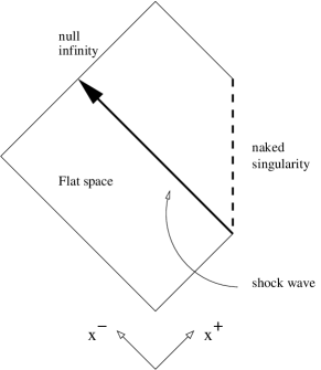
Figure 1: The naked singularity formed by the shock wave.

The flux is computed by integrating the probability over the coordinate frequency $\tilde{\omega}=\omega/\sigma$, with the density of states measure $\frac{1}{2\pi}d\tilde{\omega}$, giving

$$T_{++}=\frac{\Gamma_{0}}{2\pi}\int\Gamma(\sigma\tilde{\omega})\tilde{\omega}d\tilde{\omega}=\Gamma_{0}\frac{(\lambda^{2}x^{-}-a)^{2}}{2\pi^{3}\sigma^{2}}\;.$$ (5.4)

Similarly, in order to find the outgoing flux we integrate along $x^{-}$ starting from the naked singularity, this time using $\partial_{+}I=0$. A similar calculation first gives

$$\Im I=\frac{\pi\omega}{2\lambda^{2}x^{+}}\;.$$ (5.5)

Then, integrating the probability over the coordinate frequency, the outgoing flux

$$T_{--}=\Gamma_{0}\frac{\lambda^{4}(x^{+})^{2}}{2\pi^{3}\sigma^{2}}$$ (5.6)

is obtained (strictly speaking the outgoing flux would be $2T_{++}-2T_{--}$). The conservation equations

$$\sigma\partial_{+}T_{--}+\partial_{-}(\sigma T_{+-}) = 0\;,$$

$$\sigma\partial_{-}T_{++}+\partial_{+}(\sigma T_{+-}) = 0\,,$$ (5.7)

will determine the components only up to arbitrary functions $B(x^{-})$ and $A(x^{+})$, respectively, corresponding to the freedom of the choice of a vacuum. For instance, requiring the fluxes to vanish in the linear dilaton vacuum fixes them uniquely. As regards $T_{+-}$, it is well known that it is given by the conformal anomaly: $T=4\sigma T_{+-}=R/24\pi$ (for one bosonic d.o.f.). Matching to the anomaly gives the pre-factor $\Gamma_{0}=\pi^{2}/24$, of order one indeed. These results agree with the one-loop calculation to be found in [28]. Note that the stress tensor diverges approaching the singularity, indicating that its resolution will not be possible within classical gravity but requires instead quantum gravity [29, 19].

We return now to the RN solution. Could it be that the naked singularity emitted particles? In the $4D$ case one easily sees that the action has no imaginary part along null trajectories either ending or beginning at the singularity. Formally this is because the Kodama energy coincides with the Killing energy in such a static manifold and there is no infinite redshift from the singularity to infinity. Even considering the metric as a genuinely two-dimensional solution, this would lead to an integral for $I$

$$I=\int\frac{\omega(r-r_{+})(r-r_{-})}{r^{2}}\,dx^{+}$$ (5.8)

where $x^{\pm}=t\pm r_{*}$, with

$$r_{*}=r+\frac{r_{+}^{2}}{r_{+}-r_{-}}\ln[(r_{+}-r)/r_{+}]-\frac{r_{+}^{2}}{r_{+}-r_{-}}\ln[(r_{-}-r)/r_{-}]=\frac{x^{+}-x^{-}}{2}\;.$$ (5.9)

But close to the singularity

$$r^{2}=(3r_{+}r_{-}/2)^{2/3}(x^{+}-x^{-})^{2/3}+\cdots$$ (5.10)

not leading to a simple pole. It is fair to say that the RN naked singularity will not emit particle in this approximation.
This seems to be coherent with QFT results. Fig. 2 depicts part of a Penrose’s diagram for the region near the singularity of RN (the left one, say).

Figure 2: Part of the Penrose diagram of the RN region close to the (left) time-like singularity.

With the customary $u=x^{-}$ and $v=x^{+}$, the map $u\to v=G(u)$ gives that ingoing null geodesics which after reflection in the origin emerges as the outgoing geodesic drawn. According to [30], the radiated $s$–wave power of a minimally coupled scalar field is given in terms of the map $G(u)$ and its derivatives, by the Schwarzian derivative

$$W=\frac{1}{24\pi}\left[\frac{3}{2}\left(\frac{G^{{}^{\prime\prime}}}{G^{{}^{\prime}}}\right)^{2}-\frac{G^{{}^{\prime\prime\prime}}}{G^{{}^{\prime}}}\right]\;.$$ (5.11)

The $(u,v)$ section of the RN metric is conformally flat, hence the above map is trivial (or linear) and $W=0$.

6 Conclusions

In this paper, several applications of the tunneling method have been presented. In our opinion, the most pleasant aspect of the semi-classical tunneling method in the analyzed context is its flexibility and the wide range of situations to which it can be applied. Normally great efforts are needed to analyze quantum effects in gravity, while the tunneling picture promptly gives strong indications of what could happen. The obtained agreement between the particle decay rates from tunneling methods with the asymptotic of the exact results, when they exist in particular backgrounds like dS space, gives confidence of their validity in more general situations. Similarly, the coincidence of the tunneling radiation from naked singularities with one-loop quantum field theory results gives confidence that similar effects also exists for naked singularities in $4D$ backgrounds. In particular we have shown that the same expression derived from the Hamilton–Jacobi equation can handle several quantum effects: radiation from dynamical horizons, both cosmological and collapsing, gravitational enhancement of particle decay which would otherwise be forbidden by conservation laws, and radiation from naked singularities, at least in some $2D$ dilaton gravity models.

References

- [1] A. G. Riess et al. Astron. J. 116, 1009 (1998).
- [2] S. Perlmutter et al. Astrophys. J. 517, 565 (1999).
- [3] A. M. Polyakov, arXiv:0912.5503 [hep-th].
- [4] G. E. Volovik, JETP Lett. 90, 1 (2009).
- [5] G. Borner and H. P. Durr, Il Nuovo Cimento, Vol. LXIV A, No. 3 (1969); R. Bousso, A. Maloney and A. Strominger, Phys. Rev. D65, 104039 (2002); Y. B. Kim, C. Y. Oh and N. Park, arXiv:hep-th/0212326; E. Lifshitz, J. Phys. (USSR) 10,116 (1946); E. Mottola, Phys. Rev. D31, 754 (1985).
- [6] N. P. Myhrvold, Phys. Rev. D 28, 2439 (1983).
- [7] D. Boyanovsky, H. J. de Vega and N. G. Sanchez, Phys. Rev. D 71, 023509 (2005).
- [8] A. M. Polyakov, Nucl. Phys. B797 (2008), 199; E. T. Akhmedov, P. V. Buividovich and D. A. Singleton, arXiv: 0905.2742 [gr-qc]; E. T. Akhmedov, arXiv: 0909.3722 [hep-th].
- [9] J. Bros, H. Epstein and U. Moschella, JCAP 0802, 003 (2008) ; J. Bros, H. Epstein and U. Moschella, arXiv: 0812.3513 [hep-th]; J. Bros, H. Epstein, M. Gaudin, U. Moschella and V. Pasquier, arXiv: 0901.4223 [hep-th].
- [10] M. Angheben, M. Nadalini, L. Vanzo and S. Zerbini, JHEP 0505, 014 (2005); M. Nadalini, L. Vanzo and S. Zerbini, J. Physics A: Math. Gen. 39, 6601 (2006).
- [11] R. Kerner and R. B. Mann, Phys. Rev. D 73, 104010 (2006).
- [12] R. Di Criscienzo, M. Nadalini, L. Vanzo, S. Zerbini and G. Zoccatelli, Phys. Lett. B657, 107 (2007).
- [13] H. Kodama, Prog. Theor. Phys. 63, 1217 (1980).
- [14] S. A. Hayward, Class. Quant. Grav. 15, 3147 (1998).
- [15] S. A. Hayward, R. Di Criscienzo, L. Vanzo, M. Nadalini and S. Zerbini, Class. Quant. Grav. 26 , 062001 (2009).
- [16] R. Di Criscienzo, S. A. Hayward, M. Nadalini, L. Vanzo and S. Zerbini, Class. Quant. Grav. 27, 015006 (2010).
- [17] T. Harada, H. Iguchi and K. i. Nakao, Prog. Theor. Phys. 107, 449 (2002).
- [18] R. Casadio and B. Harms, Int. J. Mod. Phys. A 17, 4635 (2002) [arXiv:hep-th/0110255].
- [19] H. Iguchi and T. Harada, Class. Quant. Grav. 18, 3681 (2001) [arXiv:gr-qc/0107099].
- [20] M. K. Parikh and F. Wilczek, Phys. Rev. Lett. 85, 5042 (2000).
- [21] M. Visser, Int. J. Mod. Phys. D12, 649 (2003); A. B. Nielsen and M. Visser, Class. Quant. Grav. 23, 4637 (2006).
- [22] P. Menotti, arXiv: 0911.4358 [hep-th].
- [23] G. E. Volovik, arXiv: 0803.3367 [gr-qc].
- [24] S. F. Wu, B. Wang, G. H. Yang and P. M. Zhang, Class. Quant. Grav. 25, 235018 (2008).
- [25] R. Brout, G. Horwitz and D. Weil, Phys. Lett. B 192, 318 (1987).
- [26] C. Martinez, R. Troncoso and J. Zanelli, Phys. Rev. D67, 024008 (2003).
- [27] M. Nadalini, L. Vanzo and S. Zerbini, Phys. Rev. D77, 024047 (2008).
- [28] C. Vaz and L. Witten, Phys.Lett. B325, 27 (1994).
- [29] T. Harada, H. Iguchi, K. i. Nakao, T. P. Singh, T. Tanaka and C. Vaz, Phys. Rev. D 64, 041501 (2001).
- [30] L. H. Ford and L. Parker, Phys. Rev. D 17, 1485 (1978).