Quantum-tunneling dynamics of a spin-polarized Fermi gas in a double-well potential

Abstract

We study the exact dynamics of a one-dimensional spin-polarized gas of fermions in a double-well potential at zero and finite temperature. Despite the system is made of non-interacting fermions, its dynamics can be quite complex, showing strongly aperiodic spatio-temporal patterns during the tunneling. The extension of these results to the case of mixtures of spin-polarized fermions in interaction with self-trapped Bose-Einstein condensates (BECs) at zero temperature is considered as well. In this case we show that the fermionic dynamics remains qualitatively similar to the one observed in absence of BEC but with the Rabi frequencies of fermionic excited states explicitly depending on the number of bosons and on the boson-fermion interaction strength. From this, the possibility to control quantum fermionic dynamics by means of Feshbach resonances is suggested.

I Introduction

The control and manipulation of confined ultracold atomic gases make possible the study of the dynamics of many-body quantum states either for bosons folling ; spielman ; salger ; trotzky ; wurtz and for fermions shin ; inguscio , as well as for their mixtures. Ultracold atoms give the opportunity to investigate the most important quantum effects with a very high level of control and precision pitaevskii ; dalfovo ; pethick ; leggett . Among these effects, the quantum tunneling is a topic of wide interest. In this sense, one of the most important examples is provided by Bose gases confined in double-well shaped potentials. In these systems the tunneling of bosons through the central barrier, which separates the two potential wells, is responsible for the atomic counterpart of the Josephson effect (see, for instance, Refs. leggett ; smerzi ; albiez ; mazzarella ) observed in superconductive junctions book-barone . The macroscopic quantum tunneling was studied also with two weakly-linked superfluids made of interacting fermionic atoms for which it is possible to obtain atomic Josephson junction equations salasnich1 .

The optical lattices and double-well traps are paradigmatic external potentials to understand the tunneling in atomic systems characterized by a small number of particles folling ; trotzky ; esteve . The dynamics of small systems of spinless bosons zollner , of finite Fermi-Hubbard and Bose-Hubbard systems ziegler , and of spin $1/2$ fermions - especially within the quantum information community lewenstein ; cirac - were widely studied.

In this work we consider a one-dimensional (1D) dilute and ultracold gas of spin-polarized fermionic atoms in a double-well potential in the absence and in the presence of a Bose-Einstein condensate (BEC) which is intrinsically localized in one of the two potential wells. In both cases we have that in correspondence to certain values of the parameters of the double-well potential, its eigenspectrum is organized in doublets spaced between themselves and made of quasi-degenerate states. Each doublet is characterized by its own Rabi frequency, proportional to the gap between the two corresponding states. It turns out that even in absence of BEC and of interactions between the fermions, this kind of system exhibits an interesting behavior.

In the first part of the paper we focus on a spin-polarized quantum gas in absence of BEC. We suppose that at the initial time the system is prepared in such a way that all the fermions are localized at a given side of the barrier and that a number of fermionic states can be excited by means of external resonant fields (e.g. resonant with the Rabi frequencies of the doublets). The dynamics sustained by the above Hamiltonian allows to study the transfer of matter which takes place through the barrier by tunneling. This effect was studied in Ref. zollner for few bosons in a 1D double-well at zero-temperature. Indeed, the non-interacting pure fermionic system can be viewed as a realization in the infinitely strong repulsive interaction limit of 1D hard-core bosonic systems grd , where the Pauli exclusion principle mimics the hard-core interaction. By following Ref. zollner , we fix the number of fermions and analyze the spatial variations of the density profile of the fermionic cloud at different times, and the total fermionic fractional imbalance $Z_{F}$ between the two wells as a function of time $t$. We carry out this analysis both with one fermion and with more fermions by pointing out the striking differences between the two cases. In the former case the temporal behavior of $Z_{F}(t)$ is fully periodic and its period (Rabi period) is given by the inverse Rabi frequency of the lowest doublet. In the latter case the periodicity occurs on much longer times, equal to the minimum common multiple of the Rabi periods of the populated doublets. $Z_{F}(t)$ may even be completely aperiodic if some of the Rabi periods of the populated doublets are incommensurate. In any case, the shape of the density profile generally exhibits spatio temporal patterns which do not replicate the initial situation for rather long times. In Refs. zollner ; ziegler , the atomic systems therein considered are dealt with at zero-temperature. Here we perform our analysis also at nonzero temperature. By keeping fixed the number of fermions, we study the influence of the temperature on the total fractional imbalance: there is a spatial broadenings of the density profile that become more evident by increasing the temperature.

In the second part of the paper we discuss the case of a spin-polarized quantum Fermi gas interacting with a quasi-stationary BEC at zero temperature. In particular, we show that for a self-trapped BEC (e.g. a BEC intrinsically localized by the nonlinearity in one of the two wells of the potential) and for small boson-fermion interactions, the fermionic imbalance dynamics remains qualitatively similar to the one of the pure fermionic case with the only difference that the spacings of the fermionic levels (and therefore the Rabi frequencies) become dependent on both the number of bosons and the boson-fermion interaction. This suggests the possibility to control the fermionic quantum dynamics by changing, for example, the inter-species scattering lengths by using Feshbach resonances, a fact which could be of interest for applications to quantum computing.

II The system

We consider a confined dilute and ultracold spin-polarized gas of $N_{F}$ fermionic atoms of mass $m$ in a double-well potential. For dilute and ultracold atoms the only active channel of the inter-atomic potential is the s-wave scattering. For spin-polarized fermions the s-wave channel is inhibited by statistics and consequently the system is practically an ideal Fermi gas. The trapping potential of the system is given by

$$V({\bf r})=U(x)+{1\over 2}m\omega_{\bot}^{2}(y^{2}+z^{2})\;,$$ (1)

We suppose that the system is one-dimensional (1D), due to a strong radial transverse harmonic confinement flavio1 ; flavio2 , with a symmetric double-well trapping potential in the longitudinal axial direction, that we will denote by $U(x)$. We are thus assuming that the transverse energy $\hbar\omega_{\bot}$ of the confinement is much larger than the characteristic energy of fermions in the axial direction flavio1 ; flavio2 .

On the basis of the dimensional reduction, the 1D Hamiltonian of the dilute spin-polarized Fermi gas confined by the potential $U(x)$ is

$${\hat{H}}=\int{\hat{\psi}}^{\dagger}(x)\left[-{\hbar^{2}\over 2m}{\partial^{2}\over\partial x^{2}}+U(x)\right]{\hat{\psi}}(x)\ dx\;,$$ (2)

where ${\hat{\psi}}(x)$ and ${\hat{\psi}}^{\dagger}(x)$ are the usual field operators annihilating or creating a fermion at position $x$, therefore obeying anticommutation rules. The single-particle stationary Schrödinger equation associated to the Hamiltonian (2) can be written as

$$\left[-{\hbar^{2}\over 2m}{\partial^{2}\over\partial x^{2}}+U(x)\right]\phi_{\alpha,j}(x)=\epsilon_{\alpha,j}\phi_{\alpha,j}(x)\;,$$ (3)

where $\phi_{\alpha,j}(x)$ are the complete set of orthonormal eigenfunctions and $\epsilon_{\alpha,j}$ the corresponding eigenenergies. Here $\alpha=1,2,3,...$ gives the ordering number of the doublets of quasi-degenerate states, and $j=S,A$ gives the symmetry of the eigenfunctions ($S$ means symmetric and $A$ means anti-symmetric). It follows that the eigenvalues are ordered in the following way: $\epsilon_{1,S}<\epsilon_{1,A}<\epsilon_{2,S}<\epsilon_{2,A}<\epsilon_{3,S}<\epsilon_{3,A}<...\$. Without loss of generality, we consider real eigenfunctions $\phi_{\alpha,i}(x)$.

Due to the symmetry of the problem, it is useful to introduce a complete set of orthonormal functions

$$\xi_{\alpha,R}(x)={1\over\sqrt{2}}\big{(}\phi_{\alpha,S}(x)+\phi_{\alpha,A}(x)\big{)}\;,$$ (4)

and

$$\xi_{\alpha,L}(x)={1\over\sqrt{2}}\big{(}\phi_{\alpha,S}(x)-\phi_{\alpha,A}(x)\big{)}\;.$$ (5)

If we fix the phase of $\phi_{\alpha,S}$ and $\phi_{\alpha,A}$, such that $\phi_{\alpha,j}^{\prime}(+\infty)<0$ for both $j=S$ and $j=A$ then $\xi_{\alpha,L}$ and $\xi_{\alpha,R}$ are mainly localized in the left and right well respectively, at least for the low lying states.

The field operator ${\hat{\psi}}(x)$ can be written as

$${\hat{\psi}}(x)=\sum_{\alpha=1}^{\infty}\sum_{i=L,R}\xi_{\alpha,i}(x)\ {\hat{c}}_{\alpha,i}\;,$$ (6)

in terms of the single-particle fermi operators ${\hat{c}}_{\alpha,i}$ (${\hat{c}}^{\dagger}_{\alpha,i}$) satisfying the usual anticommutation rules, which destroy (create) one fermion in the state $\xi_{\alpha,L}(x)$ or $\xi_{\alpha,R}(x)$.

By inserting Eq. (6) into (2), the Hamiltonian takes the form

$${\hat{H}}=\sum_{\alpha=1}^{\infty}\sum_{i=L,R}{\bar{\epsilon}}_{\alpha}\ {\hat{c}}_{\alpha,i}^{\dagger}{\hat{c}}_{\alpha,i}-\sum_{\alpha=1}^{\infty}J_{\alpha}({\hat{c}}^{\dagger}_{\alpha,L}{\hat{c}}_{\alpha,R}+{\hat{c}}^{\dagger}_{\alpha,R}{\hat{c}}_{\alpha,L})\;,$$ (7)

where ${\hat{n}}_{F,\alpha,i}={\hat{c}}^{\dagger}_{\alpha,i}{\hat{c}}_{\alpha,i}$ is the fermionic number operator of the $\alpha$-th state in the $i$ well ($i=L,R$: $L$ means left and $R$ means right). Notice that the diagonal part of the Hamiltonian (7), given by

$${\hat{H}}_{0}=\sum_{\alpha=1}^{\infty}\sum_{i=L,R}{\bar{\epsilon}}_{\alpha}\ {\hat{c}}_{\alpha,i}^{\dagger}{\hat{c}}_{\alpha,i}\;,$$ (8)

describes a double-well Fermi system with an infinite barrier, i.e. with zero hopping terms. The energy

$${\bar{\epsilon}}_{\alpha}={\epsilon_{\alpha,S}+\epsilon_{\alpha,A}\over 2}\;$$ (9)

given by

$$\int\xi_{\alpha,i}(x)\left[-{\hbar^{2}\over 2m}{\partial^{2}\over\partial x^{2}}+U(x)\right]\xi_{\alpha,i}(x)\ dx\;,$$ (10)

is the same for the left and right states described by $\xi_{\alpha,L}(x)$ and $\xi_{\alpha,R}(x)$ The energy

$$J_{\alpha}={\epsilon_{\alpha,A}-\epsilon_{\alpha,S}\over 2}$$ (11)

is the energy of hopping from the $L$ to the $R$ well within the same doublet and gives directly half of the Rabi frequency of the $\alpha$-th doublet as

$$\Omega_{\alpha}=\frac{J_{\alpha}}{\hbar}\;,$$ (12)

i.e. the Rabi angular frequency $\Omega_{\alpha}^{Rabi}$ is given by $\Omega_{\alpha}^{Rabi}=2\Omega_{\alpha}=2J_{\alpha}/\hbar$ sakurai .

III Tunneling dynamics of free fermions in double well potential

To study the dynamics sustained by the Hamiltonian (7), we analyze the problem within the Heisenberg picture. The Heisenberg equation of motion for the operator ${\hat{\psi}}(x,t)$ is

$$i\hbar{\partial\over\partial t}{\hat{\psi}}(x,t)=[{\hat{\psi}}(x,t),{\hat{H}}]=\left[-{\hbar^{2}\over 2m}{\partial^{2}\over\partial x^{2}}+U(x)\right]{\hat{\psi}}(x,t)\;,$$ (13)

and the time-dependent density operator is

$${\hat{n}}_{F}(x,t)={\hat{\psi}}^{\dagger}(x,t){\hat{\psi}}(x,t)\;.$$ (14)

The Heisenberg equations of motion for the operators ${\hat{n}}_{F,\alpha,L}$ and ${\hat{n}}_{F,\alpha,R}$ read

$$i\hbar\frac{d}{dt}{\hat{n}}_{F,\alpha,L} = -J_{\alpha}({\hat{h}}_{\alpha,L}-{\hat{h}}_{\alpha,R})\;,$$ (15)

$$i\hbar\frac{d}{dt}{\hat{n}}_{F,\alpha,R} = J_{\alpha}({\hat{h}}_{\alpha,L}-{\hat{h}}_{\alpha,R})\;,$$ (16)

where ${\hat{h}}_{\alpha,L}={\hat{c}}^{\dagger}_{\alpha,L}{\hat{c}}_{\alpha,R}$, and ${\hat{h}}_{\alpha,R}={\hat{c}}^{\dagger}_{\alpha,R}{\hat{c}}_{\alpha,L}$. The equations of motion for the operators ${\hat{h}}_{\alpha,L}$ and ${\hat{h}}_{\alpha,R}$ are

$$i\hbar\frac{d}{dt}{\hat{h}}_{\alpha,L} = -J_{\alpha}({\hat{n}}_{F,\alpha,L}-{\hat{n}}_{F,\alpha,R})\;,$$ (17)

$$i\hbar\frac{d}{dt}{\hat{h}}_{\alpha,R} = J_{\alpha}({\hat{n}}_{F,\alpha,L}-{\hat{n}}_{F,\alpha,R})\;.$$ (18)

We want to analyze the spatio-temporal evolution of our system both at zero and finite temperature $T$. To this end, we evaluate the thermal average of both sides of the Heisenberg equations of motion obtained so far. The thermal average of an operator ${\hat{A}}(t)$ is given by

$$\langle{\hat{A}}(t)\rangle={Tr\Big{[}{\hat{A}}(t){\hat{\rho}}_{0}\Big{]}\over Tr\Big{[}{\hat{\rho}}_{0}\Big{]}}=A(t)\;,$$ (19)

where ${\hat{\rho}}_{0}$ is the chosen statistical density operator. It is clear that a thermal average evaluated by using the density operator ${\hat{\rho}}=e^{-\beta({\hat{H}}-\mu{\hat{N}})}$ (with $\beta=1/(k_{B}T)$) does not give rise to dynamics (time-dependent observables) girardeau2 . We want a statistical operator ${\hat{\rho}}_{0}$ which produces the initial conditions

$$n_{F,\alpha,L}(0)=\langle{\hat{n}}_{F,\alpha,L}(0)\rangle=f_{\alpha,L}\;,$$ (20)

$$n_{F,\alpha,R}(0)=\langle{\hat{n}}_{F,\alpha,R}(0)\rangle=f_{\alpha,R}\;,$$ (21)

with $0\leq f_{\alpha,L}\leq 1$ and $0\leq f_{\alpha,R}\leq 1$ parameters fixed by the choice of the statistical density operator. We remark that $f_{\alpha,L}$ and $f_{\alpha,R}$ can be any distribution. In particular they could be the initial distributions corresponding to thermal equilibrium in the two fully separate wells with different number of particles in each well. In this case the statistical density operator is

$${\hat{\rho}}_{0}=e^{-\beta\,({\hat{H}}_{0}-\mu_{F,L}{\hat{N}}_{F,L}-\mu_{F,R}{\hat{N}}_{F,R})}\ \;,$$ (22)

where ${\hat{H}}_{0}$ is given by Eq. (8), ${\hat{N}}_{F,i}=\sum_{\alpha=1}^{\infty}{\hat{n}}_{F,\alpha,i}$ and $\mu_{F,i}$ the number operator and the chemical potential of fermions in the $i$-th well, respectively. In this way we find

$$f_{\alpha,L}={1\over e^{\beta\,({\bar{\epsilon}}_{\alpha}-\mu_{F,L})}+1}\;,$$ (23)

$$f_{\alpha,R}={1\over e^{\beta\,({\bar{\epsilon}}_{\alpha}-\mu_{F,R})}+1}\;.$$ (24)

The chemical potentials $\mu_{F,L}$ and $\mu_{F,R}$ are fixed by the number of particles in the left and right wells at time zero:

$$N_{F,L}(0)=\sum_{\alpha=1}^{\infty}{1\over e^{\beta({\bar{\epsilon}}_{\alpha}-\mu_{F,L})}+1}\;,$$ (25)

$$N_{R,L}(0)=\sum_{\alpha=1}^{\infty}{1\over e^{\beta({\bar{\epsilon}}_{\alpha}-\mu_{F,R})}+1}\;.$$ (26)

It is easy to show that the time-dependent density profile $n_{F}(x,t)$ of the Fermi system,

$$n_{F}(x,t)=\langle{\hat{\psi}}^{\dagger}(x,t){\hat{\psi}}(x,t)\rangle\;,$$ (27)

can be written as

$$n_{F}(x,t)=\sum_{\alpha=1}^{\infty}\sum_{i=L,R}n_{F,\alpha,i}(t)\ \xi_{\alpha,i}(x)^{2}\;,$$ (28)

where $n_{F,\alpha,i}(t)=\langle{\hat{n}}_{F,\alpha,i}(t)\rangle$. In addition, from Eqs. (15)-(18) it is straightforward to get the following coupled ODEs

$${\ddot{n}}_{F,\alpha,L}+2\Omega_{\alpha}^{2}\ n_{F,\alpha,L}=2\Omega_{\alpha}^{2}\ n_{F,\alpha,R}\;,$$ (29)

$${\ddot{n}}_{F,\alpha,R}+2\Omega_{\alpha}^{2}\ n_{F,\alpha,R}=2\Omega_{\alpha}^{2}\ n_{F,\alpha,L}$$ (30)

with $\Omega_{\alpha}$ given by Eq. (12).

Notice that the total number $n_{F,\alpha}=n_{F,\alpha,L}(t)+n_{F,\alpha,R}(t)$ of fermions in the $\alpha$-th doublet and the fermionic hopping number $h_{\alpha}(t)=h_{\alpha,L}(t)+h_{\alpha,R}(t)$ are both constants of motion.

It is not difficult to show that the ODEs (29) and (30) with the initial conditions (20) and (21) have the following solutions

$$n_{F,\alpha,L}(t)=f_{\alpha,L}\ \cos^{2}{(\Omega_{\alpha}t)}+f_{\alpha,R}\ \sin^{2}{(\Omega_{\alpha}t)}\;,$$ (31)

$$n_{F,\alpha,R}(t)=f_{\alpha,R}\ \cos^{2}{(\Omega_{\alpha}t)}+f_{\alpha,L}\ \sin^{2}{(\Omega_{\alpha}t)}\;.$$ (32)

The population imbalance $z_{\alpha}(t)$ within the $\alpha$-th double is

$$z_{F,\alpha}(t)=n_{F,\alpha,L}(t)-n_{F,\alpha,R}(t)=(f_{\alpha,L}-f_{\alpha,R})\ \cos{(2\Omega_{\alpha}t)}\;,$$ (33)

and the total fermionic imbalance $Z_{F}(t)$ is given by

$$Z_{F}(t)={1\over N_{F}}\sum_{\alpha=1}^{\infty}z_{\alpha}(t)={1\over N}\sum_{\alpha=1}^{\infty}(f_{\alpha,L}-f_{\alpha,R})\ \cos{(2\Omega_{\alpha}t)}\;.$$ (34)

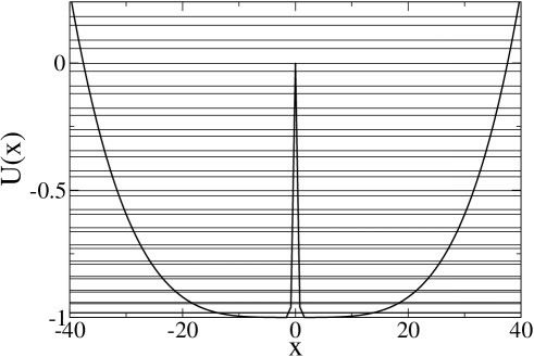
Figure 1: The double well potential (35) for $A=5\cdot 10^{-7}$, $B=1$, and $C=5$. For these values of the double-well potential parameters, there are $30$ energetic levels - corresponding to $15$ doublets - with energy smaller than the height of the barrier. Energies are measured in units of $\hbar\omega_{\bot}$, lengths in units of $a_{\bot}=\displaystyle{\sqrt{\hbar/m\omega_{\bot}}}$.

We model the double-well trapping potential $U(x)$ (see Fig. 1) in the form

$$U(x)=Ax^{4}+B(e^{-Cx^{2}}-1)\;.$$ (35)

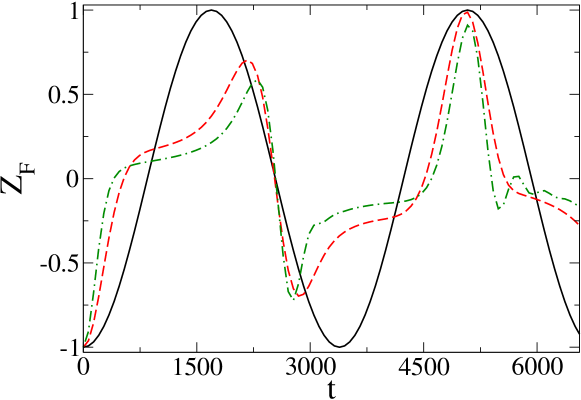
Figure 2: (Color online). Density profile $n_{F}$ vs. space $x$ and total fermionic imbalance $Z_{F}$ vs. time $t$ with $N_{F}=1$. Plots of $n_{F}(x)$ are for different values of $t$. We define $t_{1}$ as $2\pi/\Omega_{1}$. In this figure: $t=0$ and $t=0.25\,t_{1}$ (the two upper panels of $n_{F}$ from left to right); $t=0.88\,t_{1}$ and $t=1.5\,t_{1}$ (the two lower panels of $n_{F}$ from left to right). For both the $n_{F}(x)$ and $Z_{F}(t)$ plots, the continuous line represents data for $K_{B}\,T=0$, the dashed line for $K_{B}\,T=0.038$ ($\simeq(\bar{\epsilon}_{2}-\bar{\epsilon}_{1})$), and the dot-dashed line for $K_{B}T=0.087$ ($\simeq(\bar{\epsilon}_{3}-\bar{\epsilon}_{1})$). The plots at zero temperature are obtained with the fermion initially localized in the ground state of the right well; the plots at finite temperature are obtained with $N_{F,L}(0)=0$ and $N_{F,R}(0)=1$ with level occupation defined by Eq. (26). Times are measured in units of $(\omega_{\bot})^{-1}$, energies in units of $\hbar\omega_{\bot}$, and lengths in units of $a_{\bot}=\displaystyle{\sqrt{\hbar/m\omega_{\bot}}}$.

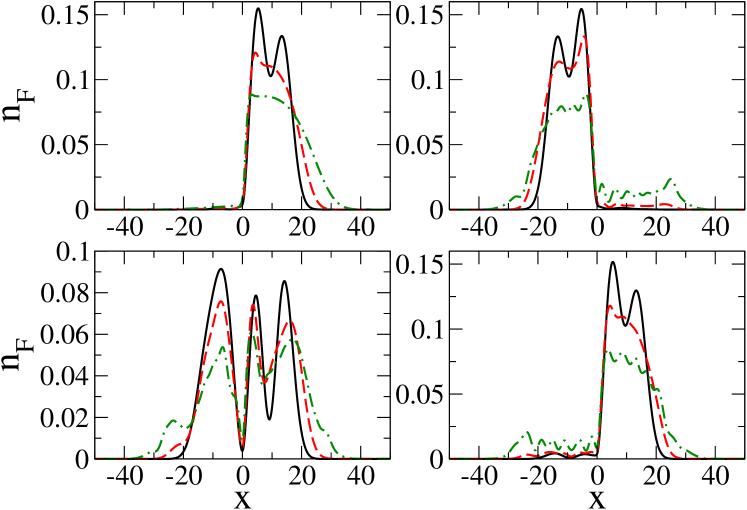
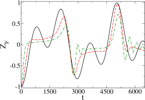
Figure 3: (Color online). Density profile $n_{F}$ vs. space $x$ and total fermionic imbalance $Z_{F}$ vs. time $t$ with $N_{F}=2$. Plots of $n_{F}(x)$ are for different values of $t$. We define $t_{1}$ as $2\pi/\Omega_{1}$. In this figure: $t=0$ and $t=0.74\,t_{1}$ (the two upper panels of $n_{F}$ from left to right); $t=0.82\,t_{1}$ and $t=1.5\,t_{1}$ (the two lower panels of $n_{F}$ from left to right). For both the $n_{F}(x)$ and $Z_{F}(t)$ plots, the continuous line represents data for $K_{B}\,T=0$, the dashed line for $K_{B}\,T=0.047$ ($\simeq(\bar{\epsilon}_{3}-\bar{\epsilon}_{2})$), and the dot-dashed line for $K_{B}\,T=0.164$ ($\simeq(\bar{\epsilon}_{5}-\bar{\epsilon}_{2})$). The plots at zero temperature are obtained with the 2 fermions initially in the 2 lower states of the right well; the plots at finite temperature are obtained with $N_{F,L}(0)=0$ and $N_{R,L}(0)=2$ with level occupation defined by Eq. (26). Units are the same as in Fig. 2.

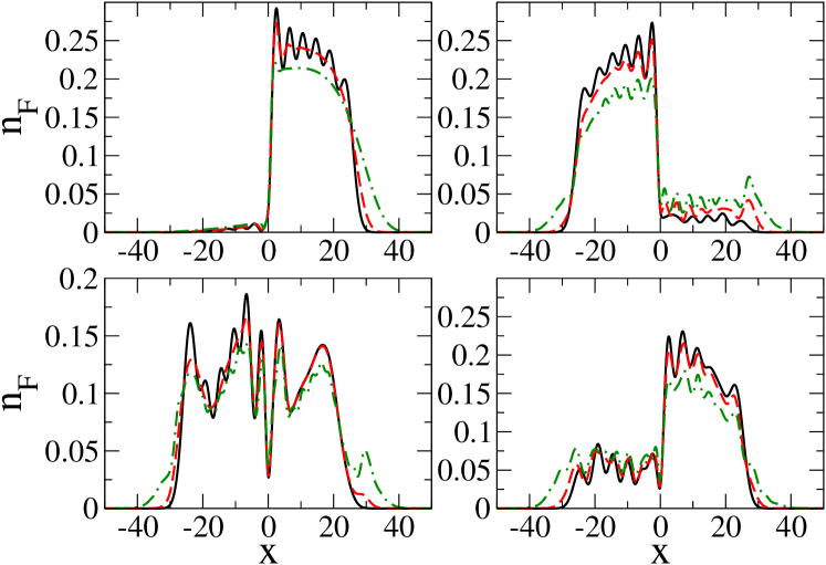
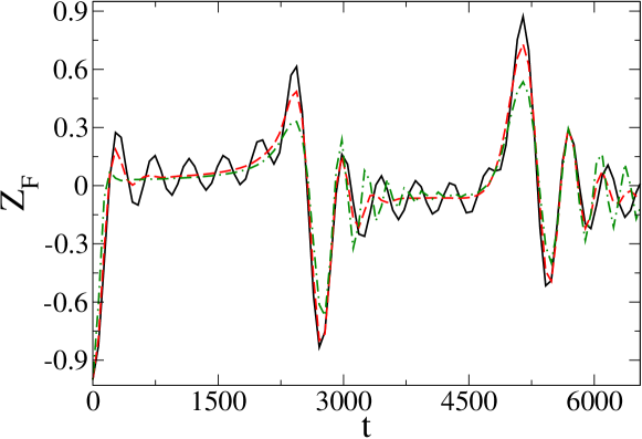
Figure 4: (Color online). Density profile $n_{F}$ vs. space $x$ and total fermionic imbalance $Z_{F}$ vs. time $t$ with $N_{F}=6$. Plots of $n_{F}(x)$ are for different values of $t$. We define $t_{1}$ as $2\pi/\Omega_{1}$. In this figure: $t=0$ and $t=0.76\,t_{1}$ (the two upper panels of $n_{F}$ from left to right); $t=0.83\,t_{1}$ and $t=1.52\,t_{1}$ (the two lower panels of $n_{F}$ from left to right). For both the $n_{F}(x)$ and $Z_{F}(t)$ plots, the continuous line represents data for $K_{B}\,T=0$, the dashed line for $K_{B}\,T=0.068$ ($\simeq(\bar{\epsilon}_{7}-\bar{\epsilon}_{6})$), and the dot-dashed line for $K_{B}\,T=0.219$ ($\simeq(\bar{\epsilon}_{9}-\bar{\epsilon}_{6})$). The plots at zero temperature are obtained with the 6 fermions initially in the 6 lower states of the right well; the plots at finite temperature are obtained with $N_{F,L}(0)=0$ and $N_{R,L}(0)=6$ with level occupation defined by Eq. (26). Units are the same as in Fig. 2.

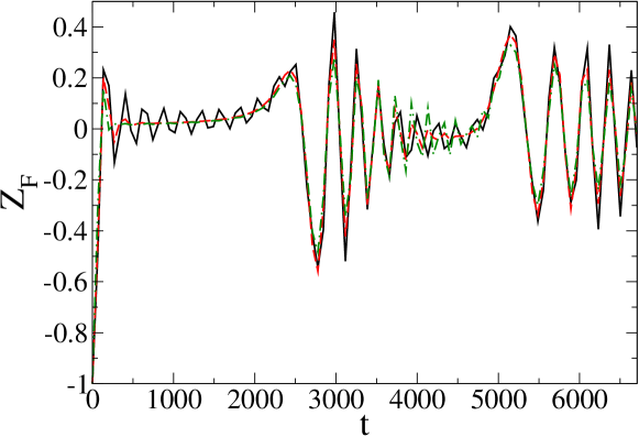
Figure 5: (Color online). Density profile $n_{F}$ vs. space $x$ and total fermionic imbalance $Z_{F}$ vs. time $t$ with $N_{F}=12$. Plots of $n_{F}(x)$ are for different values of $t$. We define $t_{1}$ as $2\pi/\Omega_{1}$. In this figure: $t=0$ and $t=0.77\,t_{1}$ (the two upper panels of $n_{F}$ from left to right); $t=0.83\,t_{1}$ and $t=1.52\,t_{1}$ (the two lower panels of $n_{F}$ from left to right). For both the $n_{F}(x)$ and $Z_{F}(t)$ plots, the continuous line represents data for $K_{B}\,T=0$, the dashed line for $K_{B}\,T=0.142$, ($(\bar{\epsilon}_{13}-\bar{\epsilon}_{12})<K_{B}\,T<(\bar{\epsilon}_{14}-\bar{\epsilon}_{12})$), and the dot-dashed line for $K_{B}\,T=0.333$, ($(\bar{\epsilon}_{15}-\bar{\epsilon}_{12})<K_{B}\,T<(\bar{\epsilon}_{16}-\bar{\epsilon}_{12})$). The plots at zero temperature are obtained with the 12 fermions initially in the 12 lower states of the right well; the plots at finite temperature are obtained with $N_{F,L}(0)=0$ and $N_{R,L}(0)=12$ with level occupation defined by Eq. (26). Units are the same as in Fig. 2.

We study the time-dependent density profile (27) and the total fermionic imbalance (34) both at zero and finite temperature for different number of fermions. The results of this study are shown in Fig. 2 ($N_{F}=1$), Fig. 3 ($N_{F}=2$), Fig. 4 ($N_{F}=6$), and Fig. 5 ($N_{F}=12$).

In our calculations we have supposed that the fermions of the system are ⁴⁰K atoms, and set the harmonic transverse frequency $\omega_{\bot}$ to $160$ kHz, so that $a_{\bot}\simeq 0.1\mu$ m flavio2 . The absolute temperatures used in Figs. 2-5 are calculated according to the above assumptions. In each of these figures we show, for fixed values of $T$, the spatial evolution of $n_{F}(x,t)$ at different times and the temporal evolution of $Z_{F}$. When $N_{F}=1$ and $T=0$ - the continuous line of Fig. 2 - only the lowest doublet is involved in the dynamics. At zero temperature, the temporal behavior of $Z_{F}$ is harmonic and is characterized by only one frequency: $2\Omega_{1}$. At finite temperatures - the dashed and the dot-dashed lines of Fig. 2 - the fermions are allowed to partially occupy doublets which are empty at $T=0$ (see the captions of Fig. 2), and the harmonicity of $Z_{F}$ is deformed by this thermal effect, as we can see from the $Z_{F}$ panel of Fig. 2.

When the number of fermions is greater than one (Figs. 3-5), doublets other than the lowest one are involved in the dynamics. At $T=0$ the temporal evolution of the total fractional imbalance - the continuous line of the $Z_{F}$ plots - is no more characterized by a single frequency as in the $N_{F}=1$ case; it is, in fact, characterized by a mixing of frequencies, each of them proportional to the gap of the corresponding filled doublet. As in the $N_{F}=1$ case, at finite temperatures the fermions can partially occupy doublets higher in energy than those filled at $T=0$ (see the captions of Figs. 3-5). The effect is to induce a deformation in the oscillations of the total fermionic fractional imbalance - with respect to $T=0$ case - as shown in the plots of $Z_{F}$ - the dashed and the dot-dashed lines - of Figs. 3-5. The thermal effects influence the fermionic density profile as well. In particular, when the temperature is finite, $n_{F}(x)$ experiences a broadening with respect to the case $T=0$. From the plots of $n_{F}$ shown in Figs. 2-5, we see that the higher is the temperature the wider is this broadening.

Finally, it is worth observing that during the dynamics of our model the system is not in thermal equilibrium and it will never reach it since the particles do not interact between themselves. Each doublet preserves its energy and its number of particles.

IV Tunneling dynamics of spin-polarized fermions interacting with intrinsically localized BEC

In this section we consider the case of a spin-polarized quantum Fermi gas in interaction with a BEC which is intrinsically localized in one of the two wells of the potential (35) at zero-temperature. In particular, we are interested in the changes in the Rabi frequencies and in the fermionic imbalance dynamics induced by the presence of the BEC. To this regard we restrict, for simplicity, to the case of a small number of excited fermionic states present in the fermionic density and to weak boson-fermion interactions. In this situation the condensate will remain self-trapped (practically stationary) in the course of time and the fermionic imbalance dynamics will be qualitatively similar to the one discussed in the previous section. The fermionic spectrum and the Rabi frequencies, however, will depend on the boson-fermion interaction due to the presence of a bosonic effective potential in the fermionic Schrödinger equation of motion (see below).

To describe the spin-polarized fermionic gas in interaction with the BEC we adopt a mean field description for the condensate but treat the fermions still quantum mechanically. In this case one can show karpiuk ; ms05 that the dynamics of the mixture is described by the following set of coupled equations

$$i\hbar\frac{\partial\Psi}{\partial t}=\left[-\frac{\hbar^{2}}{2m}\frac{\partial^{2}}{\partial x^{2}}+U(x)+g_{B}N_{B}|\Psi|^{2}+g_{BF}n_{F}\right]\Psi\;,$$ (36)

$$i\hbar\frac{\partial\chi_{j}}{\partial t}=\left[-\frac{\hbar^{2}}{2m}\frac{\partial^{2}}{\partial x^{2}}+U(x)+N_{B}g_{BF}|\Psi|^{2}\right]\chi_{j}\;,$$ (37)

where $n_{F}(x,t)=\sum_{j=1}^{N_{F}}|\chi_{j}(x,t)|^{2}$ denotes the fermionic density with $\chi_{j}(x,t)$ ($j=1,...,N_{F})$ the set of orthonormal wave functions which satisfy Eq. (37), $\Psi(x,t)$ is the bosonic wavefunction normalized to one and such that $n_{B}(x,t)=N_{B}|\Psi(x,t)|^{2}$ is the bosonic density with $N_{B}$ the total number of bosons. The 1D interaction strengths are $g_{B}=2\hbar^{2}a_{B}/(ma_{\bot}^{2})$ and $g_{BF}=2\hbar^{2}a_{BF}/(ma_{\bot}^{2})$, with $a_{B}$ and $a_{BF}$ the boson-boson and boson-fermion s-wave scattering lengths and $a_{\bot}=\sqrt{\hbar/(m\omega_{\bot})}$ the characteristic length of the strong transverse harmonic confinement of frequency $\omega_{\bot}$ flavio1 ; flavio2 . A similar study for macroscopic quantum self-trapping Bose-Josephson junction with frozen fermions was done in kivshar09 . For simplicity, we also assumed equal masses and the same trapping potential for both bosons and fermions. The bosonic cloud is self-trapped in one of the two wells when the nonlinear strength $g_{B}N_{B}$ exceeds a certain finite critical value smerzi . This condition can be written as $|a_{B}|N_{B}/a_{\bot}>(\epsilon_{1,A}-\epsilon_{1,S})/(\hbar\omega_{\bot})$ smerzi , and it is fully satisfied in our numerical experiments.

Note that the BEC wavefunction evolves according to a nonlinear Gross-Pitaevskii equation (GPE) in which the fermionic density enters as a potential, while the fermionic dynamics is still linear with the condensate density playing the role of an additional external potential. From this it is clear that the fermionic eigenstates and eigenvalues can be well approximated by the linear Schrödinger equation

$$i\hbar\frac{\partial\chi_{j}}{\partial t}=\left[-\frac{\hbar^{2}}{2m}\frac{\partial^{2}}{\partial x^{2}}+U_{eff}(x)\right]\chi_{j}\;,$$ (38)

with the effective potential $U_{eff}(x)=U(x)+g_{BF}\bar{n}_{B}(x)$, with $\bar{n}_{B}(x)$ denoting the stationary bosonic density. We have numerically verified that indeed the bosonic cloud is practically stationary. From Eq. (38) the possibility to manipulate the fermionic dynamics by changing $N_{B}$ or the inter-species scattering length becomes evident.

Figure 6: Panel a): condensate localized wavefunction $\Psi(x)$ (top curve) corresponding to $N_{B}=470$ bosons in a double well potential and in the presence of $30$ spin polarized fermions with attractive boson-boson and boson-fermion interactions $a_{B}=-0.001$, $a_{BF}=-0.001$. Horizontal lines denote the first $30$ fermionic energy levels in the presence of the condensate while the bottom curve represents the trapping potential with parameters fixed as in Fig. 1. Panel b): lowest ten fermionic eigenfunctions $\chi_{i}(x)$ (from bottom to top) in the presence (continuous curves) and in the absence (dotted lines) of the BEC wavefunction depicted in panel a) (an offset of $0.5$ between curves has been added to avoid overlapping). Panel c): first three excited states in the presence of BEC constructed with the lowest eigenstates of panel b) (see text). An offset of $0.7$ between curves was added to avoid overlapping. Panel d): fermionic densities for 10 fermions including one (dotted line), two (dash dotted line), and three (dashed line) excited states depicted in panel c. The continuous line denote the stationary fermionic density in absence of excited states. Energies are measured in units of $\hbar\omega_{\bot}$, lengths in units of $a_{\bot}=\displaystyle{\sqrt{\hbar/m\omega_{\bot}}}$. The bosonic and fermionic wavefunctions are both normalized to one.

In order to check these predictions, we have numerically determined the stationary states of the mixture by solving in a self-consistent manner the time independent equations corresponding to Eqs. (36) and (37) ms05 for the case of attractive interactions. In Fig. 6a) we show the stationary bosonic wavefunction localized in the left well of the potential and the first $30$ fermionic stationary levels obtained in presence of BEC with the self-consistent method. Notice that the lowest levels deviate from the corresponding ones obtained in Fig. 1 and the quasi degeneracy of the lowest levels is removed due to the bosonic effective potential (in the present case the Rabi frequencies of lowest levels are increased due to the level splitting). In panel b) of Fig. 6 we show the first ten fermionic stationary wavefunctions corresponding to the lowest ten energy levels of panel a), while in panel c) we depict the first three excited (e.g. non stationary) states, $\zeta_{i}(x)$, constructed from the lowest stationary wavefunctions as: $\zeta_{i}(x)=(\chi_{2i-1}(x)+\chi_{2i}(x))/\sqrt{2}$. Note that the fermionic lowest energy eigenstate is asymmetric, having the same localization of the condensate due to the attractive Bose-Fermi interaction, while the next level has the opposite localization. This implies that the lowest excited states are not localized in the same potential well, as for the pure fermionic case considered before, but are extended between the two wells.

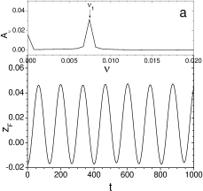
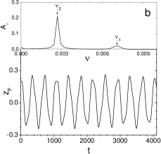
Figure 7: Panels a)-c): dynamics of the fermionic density imbalance $Z_{F}(t)$ (bottom) and corresponding Fourier spectrum (top part of panels) as obtained from numerical integrations of Eqs. (36) and (37) using as initial conditions the stationary localized bosonic wavefunction and the non stationary fermionic densities with one (a), two (b) and three (c) excited states depicted in Fig. 6. Panel d): dependence of the Rabi linear frequency $\nu_{\alpha}$ on the boson-fermion interaction for the first five excited levels indicated with dots, squares, plus, triangle and crosses, respectively. The vertical line indicates the value of $a_{BF}$ at which the other panels have been evaluated. Parameters are fixed as in Fig. 6. Time is measured in units of ${\omega_{\bot}}^{-1}$ and $a_{BF}$ is measured in units of $a_{\bot}$.

Excited fermionic densities corresponding to ten fermions and including the lowest excited states are shown in panel d) of Fig. 6 together with the stationary density. These excited densities were used, together with the BEC wavefunction shown in the top part of panel 6a), as initial conditions to calculate the total fermionic imbalance density, $Z_{F}(t)$, from direct numerical integrations of Eqs. (36) and (37). The results are depicted in Fig. 7, panels a)-c). From panel a) of this figure we see that when only one excited state is present in the density, the imbalance dynamics is periodic with a single frequency in the spectrum. The Rabi linear frequency $\nu_{\alpha}=\Omega_{\alpha}^{Rabi}/(2\pi)=\Omega_{\alpha}/\pi$ calculated from the dynamics of the fermionic imbalance density is found in very good agreement (see panel d)) with the value obtained from the energy spectrum and calculated from the nonlinear eigenvalue problem associated with Eqs. (36) and (37) using the self-consistent approach ms05 . The same good agreement is found in the case of two and three excited states present in the fermionic density panels (compare panels b),c), with corresponding values of panel d)).

From panels a)-c) of Fig. 7 it is clear that the fermionic imbalance dynamics is given by a superposition of harmonics in number equal to the number of excited states and with periods fixed by the level spacing Rabi frequencies. Also note from panel c) of Fig. 7 the presence of beatings of period $1/(\nu_{2}-\nu_{3})$ generated by the the two close frequencies $\nu_{2}$ and $\nu_{3}$, as expected for linear systems (notice also the presence of small peaks close to the Rabi brequency $\nu_{1}$ probably due to the quasi-stationarity of the bosons).

The dependence of the Rabi frequency on the Bose-Fermi interaction is depicted in Fig.7d) for the first five excited states. Note that the frequency of the first excited state has a large variation with $a_{BF}$ due to the fact that the corresponding eigenstates are the ones most effected by the presence of the condensate (see Fig. 6b). Similar dependences are also obtained by changing the number of atoms in the condensate and keeping fixed the fixed boson-fermion interaction.

From this we conclude that in the BEC self-trapped regime the dynamics for the fermionic density imbalance remains qualitatively similar to the one observed in the pure fermionic case but with the Rabi frequencies explicitly dependent on the boson-fermion interaction. Since this interaction can be easily changed by external magnetic fields via Feshbach resonances, we have found an effective way to control the the dynamics of the spin polarized fermionic gas which can be implemented in a real experiment.

V Conclusions

We have investigated a confined dilute and ultracold spin-polarized gas of fermionic atoms in a double-well potential. We have analyzed the quantum tunneling through the central barrier by studying the density profile and the total fermionic fractional imbalance. We have pointed out that despite the fermions do not interact between themselves, the dynamics is quite complex, and it exhibits very interesting aperiodicity features. We have performed our analysis both at zero and finite temperature by discussing the role of the temperature in producing deformations of the density profile with respect to the zero-temperature case. We also have discussed the possibility to include in the system a bosonic component, which, under given hypothesis, does not produce important changes in the dynamics of the system at least within very low temperature regimes. In particular, we have shown that the presence of a self trapped Bose-Einstein condensate weakly interacting with the spin-polarized fermi gas allows to achieve a quite effective control of the Rabi frequencies of excited fermionic states by changing the boson-fermion interaction with external magnetic fields via Feshbach resonances. This Bose-Einstein condensate-induced control of the fermionic quantum dynamics and can be implemented in a real experiment and can be of interest for applications to quantum computing.
This work has been partially supported by Fondazione CARIPARO through the Project 2006: ”Guided solitons in matter waves and optical waves with normal and anomalous dispersion”. MS acknowledges partial support from MIUR through a PRIN-2007 initiative.

References

- (1) S. Fölling et al., Nature 448, 1029 (2007).
- (2) I. B. Spielman, W. D. Phillips, and J. V. Porto, Phys. Rev. Lett. 98, 080404 (2007).
- (3) T. Salger, C. Geckleler, S. Kling, and M. Weitz, Phys. Rev. Lett. 99, 190405 (2007).
- (4) S. Trotzky et al., Science 319, 295 (2008).
- (5) P. Würtz, T. Gericke, A. Koglbauer, and H. Ott, Phys. Rev. Lett. 103, 080404 (2009).
- (6) Y. Shin, M. W. Zwierlein, C. H. Schunck, A. Schirotzek, and W. Ketterle, Phys. Rev. Lett. 97, 030401 (2006); G. B. Partridge, Wenhui Li, Y. A. Liao, R. G. Hulet, M. Haque, H. T. C. Stoof, Phys. Rev. Lett. 97, 190407 (2006); N. Strohmaier, Y. Takasu, K. Günter, R. Jördens, M. Köhl, H. Moritz, and T. Esslinger, Phys. Rev. Lett. 99, 220601 (2007).
- (7) Ultra-cold Fermi Gases, edited by M. Inguscio, W. Ketterle, and C. Salomon, (IOS Press, Amsterdam, 2007).
- (8) L. Pitaevskii and S. Stringari, Bose-Einstein Condensation (Oxford University Press, Oxford, 2003).
- (9) F. Dalfovo, S. Giorgini, L. Pitaevskii, and S. Stringari, Rev. Mod. Phys. 71, 463 (1999).
- (10) C. J. Pethick and H. Smith, Bose-Einstein Condensation in Dilute Gases, (Cambridge University Press, Cambridge, 2001).
- (11) A. J. Leggett and F. Sols, Found. Phys. 21, 353 (1991); I. Zapata, F. Sols, and A. J. Leggett, Phys. Rev. A 57, R28 (1998); A. J. Leggett, Rev. Mod. Phys. 73, 307 (2001).
- (12) A. Smerzi, S. Fantoni, S. Giovanazzi, and S. R. Shenoy, Phys. Rev. Lett. 79, 4950 (1997); S. Raghavan, A. Smerzi, S.Fantoni, and S. R. Shenoy, Phys. Rev. A 59, 620 (1999).
- (13) M. Albiez, R. Gati, J. Fölling, S. Hunsmann, M. Cristiani, M. K. Oberthaler, Phys. Rev. Lett. 95, 010402 (2005); R. Gati and M. K. Oberthaler, J. Phys. B: At. Mol. Opt. Phys. 40, 10, R61-R89 (2007).
- (14) G. Mazzarella, M. Moratti, L. Salasnich, M. Salerno, and F. Toigo, J. Phys. B: At. Mol. Opt. Phys. 42, 125301 (2009).
- (15) A. Barone and G. Paternò, Physics and Applications of the Josephson effect (Wiley, New York, 1982); H. Otha, in SQUID: Superconducting Quantum Devices and their Applications, edited by H.D. Hahlbohm and H. Lubbig, (de Gruyter, Berlin, 1977).
- (16) L. Salasnich, N. Manini, and F. Toigo, Phys. Rev. A 77, 043609 (2008).
- (17) J. Estéve et al., Nature 455, 1216 (2009).
- (18) S, Zöllner, H.-D. Meyer, and P. Schmelcher, Phys. Rev. Lett. 100, 040401 (2008); S, Zöllner, H.-D. Meyer, and P. Schmelcher, Phys. Rev. A 78, 013621 (2008).
- (19) K. Ziegler, e-print arXiv:0909.4932 (2009).
- (20) M. Lewenstein et al., Adv. Phys. 56, 243 (2007).
- (21) J. I. Cirac in Ultra-cold Fermi Gases, edited by M. Inguscio, W. Ketterle, and C. Salomon, (IOS Press, Amsterdam, 2007).
- (22) M. Girardeau, J. Math. Phys. (N.Y.) 1, 516 (1960).
- (23) L. Salasnich and F. Toigo, J. Low. Temp. Phys. 50, 643 (2008).
- (24) G. Mazzarella, L. Salasnich, and F. Toigo, Phys. Rev. A 79, 023615 (2009).
- (25) J.J. Sakurai, Advanced Quantum Mechanics (Addison Wesley Longman, New York, 1967).
- (26) K.K. Das, M.D. Girardeau, and E.M. Wright, Phys. Rev. Lett. 89, 170404 (2002).
- (27) S.F. Caballero Benítez, E.A. Ostrovskaya, M. Gulácsí and Yu. S. Kivshar, J. Phys. B: At. Mol. Opt. Phys. 42, 215308 (2009).
- (28) T. Karpiuk, M. Brewczyk, S. Ospelkaus-Schwarzer, K. Bongs, M. Gajda, and K. Rza̧źewski, Phys. Rev. Lett. 93, 100401 (2004); T. Karpiuk, M. Brewczyk, and K. Rza̧źewski, Phys. Rev. A 69, 043603 (2004).
- (29) M. Salerno, Phys. Rev. A 72, 063602 (2005).