The Effect of Projection on Derived Mass-Size and Linewidth-Size Relationships
Abstract
Power law mass-size and linewidth-size correlations, two of “Larson’s laws,” are often studied to assess the dynamical state of clumps within molecular clouds. Using the result of a hydrodynamic simulation of a molecular cloud, we investigate how geometric projection may affect the derived Larson relationships. We find that large scale structures in the column density map have similar masses and sizes to those in the 3D simulation (PPP). Smaller scale clumps in the column density map are measured to be more massive than the PPP clumps, due to the projection of all emitting gas along lines of sight. Further, due to projection effects, structures in a synthetic spectral observation (PPV) may not necessarily correlate with physical structures in the simulation. In considering the turbulent velocities only, the linewidth-size relationship in the PPV cube is appreciably different from that measured from the simulation. Including thermal pressure in the simulated linewidths imposes a minimum linewidth, which results in a better agreement in the slopes of the linewidth-size relationships, though there are still discrepancies in the offsets, as well as considerable scatter. Employing commonly used assumptions in a virial analysis, we find similarities in the computed virial parameters of the structures in the PPV and PPP cubes. However, due to the discrepancies in the linewidth- and mass- size relationships in the PPP and PPV cubes, we caution that applying a virial analysis to observed clouds may be misleading due to geometric projection effects. We speculate that consideration of physical processes beyond kinetic and gravitational pressure would be required for accurately assessing whether complex clouds, such as those with highly filamentary structure, are bound.
1 Introduction
Though stars form in the densest cores within much more voluminous molecular clouds, the motions and forces within the parent cloud at various scales significantly shape, if not control, the evolution of the cores as they form stars. Observations, in particular of dust emission and extinction and of a variety of molecular lines, have provided much information about the internal structure and dynamics of molecular clouds. However, determining the 3-dimensional (3D) structure of the cloud from observations is not trivial, due in large part to line-of-sight projection effects.
The scaling between the mass and velocity dispersion with size scale is often studied, in both numerical models and observations of star forming regions (e.g. Ostriker et al., 2001; Myers & Goodman, 1988; Ballesteros-Paredes & Mac Low, 2002; Dib et al., 2007; Falgarone et al., 1992; Heyer et al., 2009; Solomon et al., 1987, Kauffmann et al. 2010a,b in preparation). A radius is often considered as a proxy for the size of the region under inspection, to construct power-laws and . Larson (1981) found and , now generally known as (the first and third) “Larson’s Laws.” Larson’s second law, relating with the ratio of /, is a consequence of the other two, and is often used to study the dynamic nature of the cloud, through the virial parameter . The value of may be indicative of whether structures or other such contiguous regions within clouds are bound, due either to its own self-gravity or by the ambient external pressure (Bertoldi & McKee, 1992; McKee & Zweibel, 1992). However, assumptions about the virial theorem that are commonly employed to derive , e.g. that the surface terms are negligible compared to the volume terms, may in fact be erroneous, as discussed by Ballesteros-Paredes (2006) and Dib et al. (2007).
In order to properly interpret the Larson scaling relations, a thorough understanding of the effects of projection would be necessary. Contiguous structures in an observed position-position-velocity (PPV) cube may not be representative of actual 3D structures in position-position-position (PPP) space of the simulation(Adler & Roberts, 1992; Ostriker et al., 2001). In fact, Pichardo et al. (2000) showed that the structure of a PPV cube is more tightly correlated with the line-of-sight velocity structure than the 3D density distribution. Similarly, identified structures in a 2D (integrated emission and/or extinction) map, such as high density knots or filaments, may also be a superposition of numerous lower density peaks along the line of sight (e.g. Ostriker et al., 2001; Gammie et al., 2003). These projection effects may indeed provide power law scalings that differ from the actual scalings (as discussed by Ballesteros-Paredes et al., 1999; Ballesteros-Paredes & Mac Low, 2002).
Here, we assess the effect of projection from an analysis of a 3D numerical simulation of a molecular cloud. We compare the derived - and - relationships from 2D projected density and 3D spectral (PPV) data with those obtained from the full 3D simulation (PPP) density and velocity data. To derive , , and , we employ dendrograms, a recently developed technique which identifies contiguous structures within various chosen (intensity or density) thresholds, and in the process characterizes the hierarchical nature of the data (Rosolowsky et al., 2008). We then use the measured sizes, masses, and linewidths in a virial analysis, to extend our PPP and PPV comparison. In the next section, we briefly describe the simulation dataset and our method of analysis. In Section 3, we present the Larson relationships obtained from the full 3D simulation data and idealized observations of those simulations, and compare the results. We discuss the implications of the results in Section 4, focusing on the interpretations of observations. We summarize our findings in Section 5.
2 Method
In our investigation of the effect of projection on the derived mass- size and linewidth-size relationships, we use the result of a 3D hydrodynamic simulation at a single timestep. The simulation used for this study was run with the MHD extension of the Adaptive Mesh Refinement (AMR) code ENZO described by Collins et al. (2010). In the MHD simulation of the molecular cloud, isothermal gas collapses into filaments and eventually forms dense cores in a 1000 pc3 region, with periodic boundary conditions. The gas initially has uniform density = 200 cm-3 and magnetic field = 0.6 G, with isothermal temperature 10 K. The virial parameter for this box is 0.9, giving a slightly unstable initial cloud. At each timestep, the gas is driven with a random Gaussian velocity field. The driving field has power in a top-hat distribution between wavenumbers , and is normalized to keep the energy input constant, as described in Mac Low (1999). This results in a constant RMS mach number of 9. This driving was maintained for several dynamical times to obtain statistical independence from the initial conditions, after which self-gravity was switched on. The data analyzed in this study was taken after 0.5 free fall times.
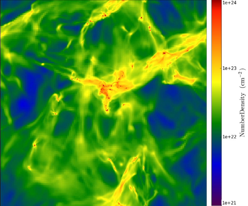
The root grid has a resolution of zones. Due to the AMR feature of the ENZO code, the resolution increases with increasing density, such that the Jeans length of the gas is always resolved by 4 zones, satisfying the Truelove criterion (Truelove et al., 1997). A total of 4 levels of refinement are added this way. Self-gravity is included, by solving the Poisson equation in the root grid using Fast Fourier Transforms, and in the subgrid patches using a multigrid technique. Normalizing the simulation to a 10 pc side length, this gives a fine grid resolution of 1000 AU. A projection of the density can be seen in Figure 1, which shows the filamentary nature of the gas. Details of this simulation will be discussed in a forthcoming paper.
A common method to locate clumps involves the identification of contiguous structures in datacubes above a chosen threshold. In algorithms such as CLUMPFIND (Williams et al., 1994), or similar variants (see e.g. Dib et al., 2007), structures are labeled as clumps if they are distinct from the background or from nearby, isolated structures. Some investigators fit Gaussian profiles to describe the shape of the structures (GAUSSCLUMP, Stutzki & Guesten, 1990). Since molecular clouds are known to be hierarchical, evidenced by observations of dense knots situated in filamentary structures within GMCs, such a method may be inadequate (Pineda et al., 2009). We thus employ “dendrograms,” a technique which characterizes the hierarchical nature of the matter distribution, while simultaneously identifying contiguous structures within chosen (intensity or density) thresholds111We we will refer to any of the structures identified by dendrograms generally as “clumps” regardless of whether they are self-gravitating (or bound) or not. (Rosolowsky et al., 2008).
The simulation data provides and the velocity components , , and at every position at a chosen time. The -cube itself contains all the information necessary to obtain the mass and size distribution of the clumps in the simulation. The mass of a clump is simply the density integrated over all zones within a dendrogram-identified region, or isosurface, in the -cube, multiplied by the volume of each zone. We regrid the result of the AMR simulation into a uniform grid with 2563 zones, each with length , so that the volume of a zone is . To characterize the size of each clump, we define a radius as that which identifies a sphere with the same volume as that bound by the isosurface, so , where is the number of zones within the dendrogram defined isosurface. We can then assess whether any clear mass-size relationship exists in the 3D simulation data.
To obtain the linewidth-size relationship of the simulation, we use the velocity information to measure the velocity dispersion of a clump. For any observation, denser gas contribute more to the observed linewidths than diffuse gas. Thus, for more direct comparison with observations, we consider the density weighted velocity dispersion. From the isosurface defined in the -cube, the corresponding velocity components , , and , as well as the density , define the 1D density-weighted velocity dispersion of that particular clump:
| (1) |
where the summation is taken over all zones constituting the identified clump. Since Equation 1 does not include the thermal velocity, it is only representative of the non-thermal, or turbulent, velocities. An observed linewidth would include a contribution from the sound speed in addition to , so
| (2) |
In our investigation of the linewidth-size relationship, we consider both the turbulent linewidth as well as the total linewidth .
In order to investigate the effect of projection, we generate a PPV cube and a column density map (shown in Figure 1) of the simulation cube. We then produce dendrogram trees of these synthetic observations, and compare the resulting mass-size and linewidth-size relationships with those obtained from the full 3D simulation data. We only consider optically thin emission, so our analysis is analogous to observational investigations involving much of the volume of the molecular cloud, including regions containing dense cores (Myers & Goodman, 1988; Falgarone et al., 1992; Heyer et al., 2009; Solomon et al., 1987; Larson, 1981). This study is thus a first step towards a complete understanding of the unavoidable consequences of projection in observations. Results based on this assumption may not be directly applicable to molecular line observations tracing high densities, such as ammonia observations of dense star forming cores. A thorough investigation of the effect of projection for those high density tracers would require the additional consideration of radiative transfer effects.
To produce a 2D column density map, we integrate the density along a given direction (e.g. ). Since we are assuming purely optically thin emission, the final 2D map is simply the zeroth-moment of the -cube. We then construct the dendrogram tree of this 2D map, obtaining the masses and sizes of each 2D-clump. In this case, we define the radius , which is the radius of a circle with an area identical to the area within the 2D isosurface.
From the simulation data, a 3D PPV cube is constructed by binning a chosen velocity component (e.g. ), and integrating the mass (e.g. along at each position) associated with each velocity bin. We consider an idealized PPV cube, with high spatial and spectral resolution of 0.039 pc and 0.025 km s-1, respectively; at these resolutions, both the density and velocity structures can be assessed to scales smaller than the typical size of the dense cores within filaments. Clump masses are obtained by integrating the intensity within each dendrogram isosurface of the PPV cubes. The velocity dispersion is obtained by computing the second moment of each clump in velocity; we will refer to this moment as , since we construct the PPV cube along the direction. We only consider clouds to by sufficiently resolved if 0.025 km s-1, which is the spectral resolution of the PPV cube (Rosolowsky & Blitz, 2005). For the clumps in the PPV cube, the observed velocity dispersion . As with the 2D map, we use the projected area associated with each clump to define as the size of the clump.
From the full simulation dataset, we derive the mass-size and linewidth-size and power law relationships of the simulated cloud. We then compare those with the , , and relationships obtained from analyses of the column density map and PPV cube.
3 Results
3.1 Mass-Size Relationships
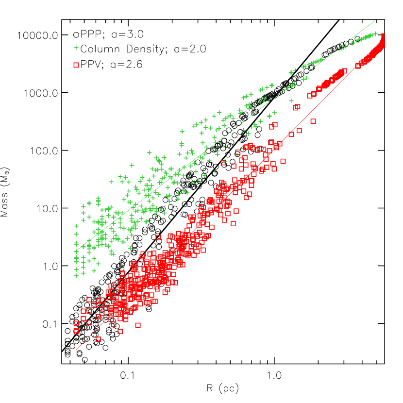
Figure 2 shows mass-size relationships of the dendrogram identified clumps, from the full 3D simulation data, the column density map, and the PPV cube. In all cases, there is a strong correlation between the and , suggestive of a power law relationship . Best fit lines give and for the 2D and 3D cases, respectively, and for the PPV cube. The best fit indices, along with the errors, are listed in Table 1; the table also indicates best fit exponents and the errors for the linewidth-size relationships discussed below.222The computed (“standard”) errors in the linear fits are small due to the very large number of datapoints. Thus, the fits provide estimates for the mean value of or with high accuracy. However, a prediction of or using an individual datapoint would have a significant error, due to the large scatter in Figures 2 - 4. The best fit mass-size indices from the column density map and the PPV cube are similar to those derived from many observations of molecular clouds (e.g. Kauffmann et al. 2010b, in preparation, Larson, 1981).
Power law fits from observations have provided an estimate (Larson, 1981; Solomon et al., 1987), known as “Larson’s 3rd Law.” Indices of and indicate that structures have constant column densities and constant volume densities in 2D and 3D, respectively. A further consequence is that the surface density is constant for all clouds.
The best fit relationships shown in Figure 2 suggest that the dendrogram identified clumps have little density variation within them. Clumps with small extents are more likely to have nearly constant (column or volume) densities, and indeed clumps with 0.6 pc generally agree well with the and relationships. Note, however, that at small scales there is still a range of clump masses at any given , indicating that the fragmentation process produces clumps with a range of masses. Larger scale clumps include contributions from the smaller, high density clumps, and so can have larger density gradients within their surfaces; as can be seen in Figure 2, those clumps deviate from the and relationships. We note that we have also modeled the clumps as ellipsoids (see e.g. Rosolowsky et al., 2008; Bertoldi & McKee, 1992), and obtain slightly different mass-size power-law indices, with and for the 2D map and PPP data, respectively; this difference indicates that the definition of plays a role in the derived mass-size relationship. Taking these issues into consideration, even though the best fit indices are and from the column density map and PPP cube, respectively, we do not conclude that the structures in the simulation have constant volume densities, or that the surface density is everywhere equivalent.
Though there are strong correlations between and at 0.5 pc, the masses derived from the 2D map are systematically larger than those from the 3D cube. As described by Gammie et al. (2003), this discrepancy arises because peaks in the 2D map may include contributions from spatially separated objects which lie along the same line of sight (see also Kauffmann et al. 2010c, ApJ Submitted, for mass contamination by extended envelopes); this blending of structures along the line of sight also results in fewer total clumps found by dendrograms in the 2D map (not all the clumps are shown in Figure 2).
For clumps with 0.5 pc, there is relatively good agreement in the masses of the 2D and 3D structures. These represent the low density, large scale structures, and their total masses include the masses of the higher density, smaller scale clumps embedded within them (i.e. the mass of the “branches” of the dendrogram tree includes the mass of any “leaves” associated with that “branch,” see Rosolowsky et al. (2008) for definitions). As the clump scale increases, the masses of both the 2D and the PPP clumps approaches the total mass of the simulated cloud.
From the PPV cube, many clumps at small scales ( 0.08 pc) have similar masses and sizes to those from the PPP data. At those scales, the clumps are the highest density objects (e.g. “cores”); many of those clumps may be detected as objects in high resolution PPV cubes since they might have velocities that are distinguishable from the surrounding material. But, some of the low mass PPV clumps are not identified as such in the PPP or column density maps; they are simply part of much larger low density features. They are identified as clumps in the PPV cube because various regions along that line-of-sight have similar (turbulent) velocities, and therefore occur as brighter knots in the PPV cube (as discussed by Pichardo et al., 2000). Thus, many of the low mass, small extent PPV clumps in Figure 2 are actually part of the larger, low density PPP clumps. Additionally, we found that for PPV cubes with lower resolution, many of the identified low mass clumps may not be detected.
At large scales, at a given radius the masses of the PPV clumps are systematically lower than those of the PPP clumps. This offset arises because of the difference in the definition of and , as well as a consequence of only including densities within given velocity bins in the construct of the PPV cube. Due to the latter effect, line of sight velocity gradients within a 3D structure may result in (1 or more) corresponding structure(s) in the PPV cube having lower mass(es) than the single 3D object; a 3D structure within a molecular cloud may thus not appear as a distinct structure in a PPV cube. These discrepancies indicate that the identification of clumps in a PPV cube may not provide accurate estimates of the masses of the real clumps.
The general agreement between the PPV and PPP masses and sizes at small scales, transitioning to lower PPV masses at a given size at larger scales, results in for the PPV clumps. A derived index between the result from the 2D analysis and from the full 3D data should be expected, since a PPV cube is constructed using the column density in defined line of sight velocity bins, thus involving a mixture of the column density and 3D density.
3.2 Linewidth-Size Relationships
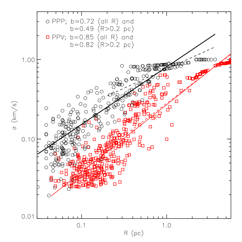
Figure 3 shows the non-thermal and relationships of dendrogram identified objects from the PPP and PPV cubes, respectively. A best fit of produces for the PPP case. For the PPV clumps, there is a large scatter in the relationship, and a best fit yields . In practice, it is difficult to accurately measure linewidths for regions smaller than a few tenths of a parsec. We thus also perform the fit only considering those structures with pc, and obtain flatter power-laws with for the PPP clumps and for the PPV clumps. Even when excluding the small scale clumps, a significant difference in the nonthermal linewidth - size relationship between the PPP and PPV cases remains.
Besides the differences in the slopes of the linewidth - size relationships, is systematically lower than the linewidth computed using all velocity components, . Both PPP and PPV dispersions are density weighted, either by design (see Eqn. [1]), or due to the intrinsic nature of a PPV cube. Thus, any discrepancy can be largely attributed to the effect of projection. For example, might include contributions from physically separate structures, since a clump in a PPV cube might consist of separate structures in the PPP cube. Additionally, for a given clump does not include any contribution from and , though it has been estimated that this can account for at most 20% of the discrepancy seen. The observed is affected by many factors besides the intrinsic velocity distribution of a given gaseous structure.
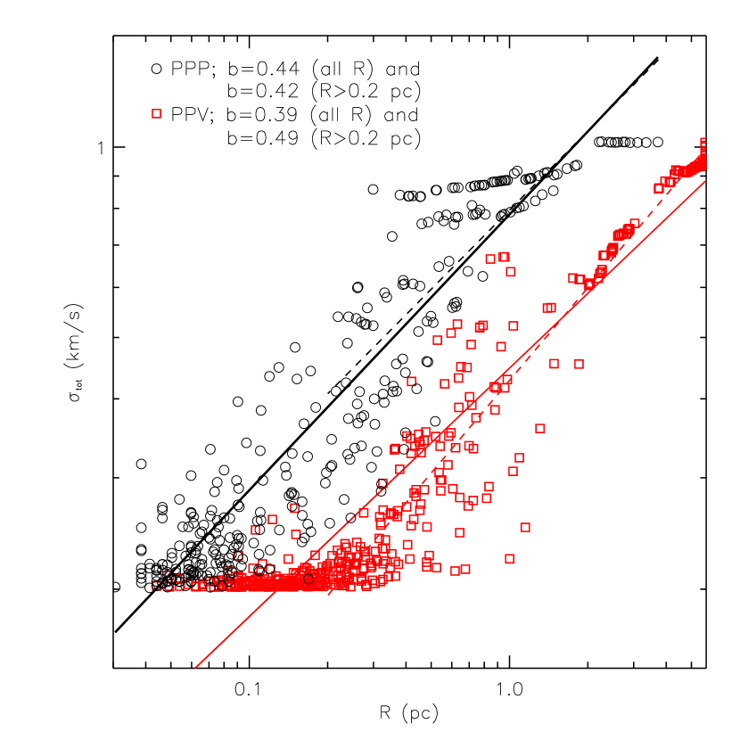
As indicated in Section 2, an observed linewidth would include a contribution from the thermal velocity; Figure 4 shows the relationship from the PPP and PPV data. At small scales, the minimum linewidths are 0.2 km s-1, which is equal to of the simulation; turbulence does not contribute much to the observed linewidths where the turbulent velocities. Compared with Figure 3, which only shows the turbulent components, the minimum linewidth imposed by the thermal component forces the power law index in the PPP and PPV case to decrease to and , respectively. For those structures with pc, best fits do not change the PPP relationship, but increases the PPV linewidth size index to , similar to results from numerous observational works (e.g. Solomon et al., 1987; Larson, 1981). Despite the better correspondence in best fit power laws, there is still a clear systematic offset between the PPP and PPV total linewidths; the best fit intercepts still differ by a factor of 2 (Figure 4, with a larger discrepancy in the turbulent offsets, as evident in Figure 3). Table 1 lists the best fit indices for the various power laws considered.
3.3 Mean Subtracted Data and 13CO Emission
We note that in a column density map where the mean density was subtracted off at each location, the resulting mass-size relationship is similar to that shown in Figure 2. The main difference is that the measured masses are slightly lower, as would be expected. The masses of the small scale clumps are still appreciably larger than those from the PPP cube. We have also performed our analysis on the simulation data where only gas above 650 cm-3 is considered to be emitting, a scenario analogous to observing optically thin 13CO. We find little difference in the derived mass-size and line-size relationships compared with the scenario where all gas is emitting. Again, the main difference is that the measured masses are slightly lower.
4 Discussion
4.1 Virial Parameters of the PPP and PPV Clumps
The observed - and - correlations have strong bearings on the interpretation of the state of the cloud, such as the bounded nature of clumps or the clouds as a whole. For example, a relationship between and can be constructed from the and relationships:
| (3) |
The relationship expressed by Equation 3 is often utilized for studying whether clumps are bound, through the virial parameter (e.g. Goodman et al., 2009; Rosolowsky et al., 2008; Larson, 1981). Clumps with 2 are considered bound, due to its own self gravity (McKee & Zweibel, 1992). For (“Larson’s 3rd law”) and (“Larson’s 1st law”), is independent of , and if its value is , the clumps under consideration are interpreted to be in, or close to, virial equilibrium (“Larson’s 2nd law,” Larson, 1981). We note, however, that a recent investigation of high resolution 13CO observations by Heyer et al. (2009) has found that structures in molecular clouds in fact do not universally follow all of “Larson laws.”
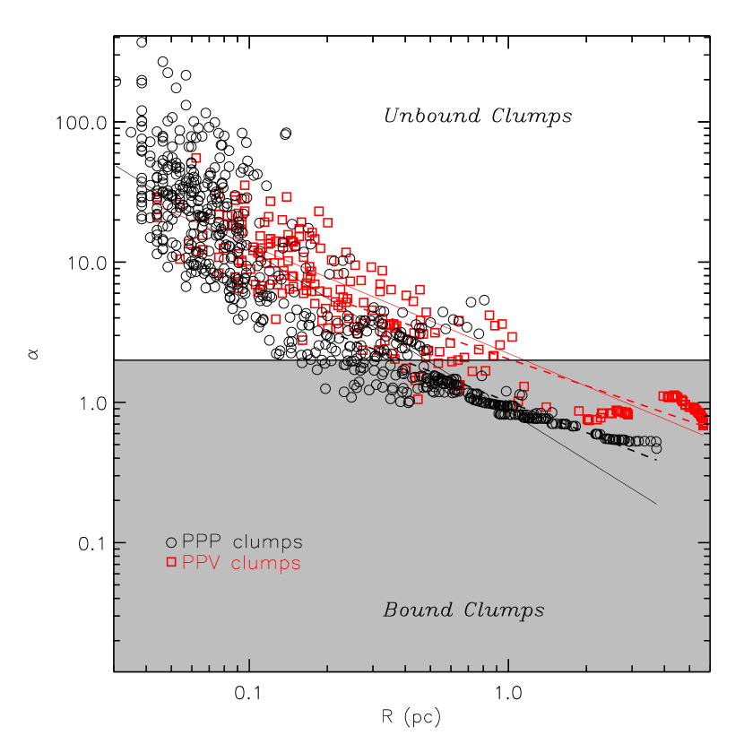
Even though we have found significant differences between the power law relationships we obtain from the PPP and synthetic observations, we carry forward an analysis to assess the stability of the clumps. Taking and from the PPP cube, . This relationship leads to . We explicitly show as a function of from the PPP analysis in Figure 5. Smaller scale clumps have 2, suggesting they are unbound. At 0.5 pc, 2, suggesting that the large scale structures are close to virialized, or are bound.
For and from the PPV analysis, . These power-laws result in . As Figure 5 illustrates, the relationships of the PPV and PPP clumps are rather similar, despite the glaring differences in the mass- and linewidth- size relationships shown in Figures 2-4. Though the trend of decreasing virial parameter with increasing radius from the PPP data is generally reproduced in the PPV analysis, the threshold radius of 1 pc beyond which clouds are bound varies significantly from the corresponding radius of the PPP clumps.
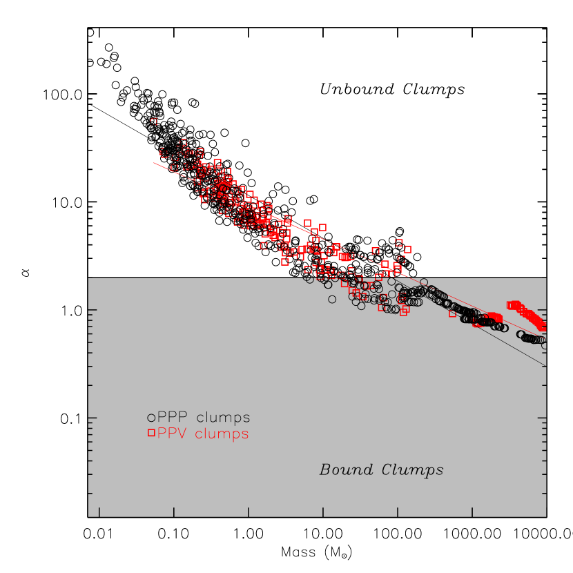
Figure 6 shows the relationship. The slopes of these power laws are 0.4 and 0.3 for the PPP and PPV clumps, respectively. Similar to the clumps in the simulations of Dib et al. (2007), the large -parameters of the low mass dense cores suggests that these objects are not bound by their own self-gravity. One interpretation of a decreasing virial parameter with radius, and of very large for the smallest scale clumps, is that dense cores are pressure confined, as formulated by Bertoldi & McKee (1992). However, our best-fit exponents differ from the 2/3 value derived for purely pressure confined clumps (Bertoldi & McKee, 1992), suggesting that other physical processes, and/or other terms in the virial equation, need to be taken into account.
The similarity in the virial parameters of the clumps from the PPP and PPV clumps must not lead to the interpretation that PPV clumps can reliably provide accurate measurements of . One reason for the general agreement is due to the abundance of low mass clumps in the PPV cube. As discussed in 3, many of these clumps in fact are not distinct objects in the simulation data.
Generally, current observations have lower resolutions than those considered in this work, and such observations would not be capable of detecting all the small scale PPV clumps shown in Figures 2 and 4. The resulting - power law would have a flatter index than the 0.8 shown in Figure 5. Further, at intermediate radii (0.1 pc 0.3 pc), there is a clear offset in the measured virial parameter of the PPV clumps compared to those of the PPP clumps, due to the lower mass estimates of the PPV clumps (see Figure 2).
Additionally, we note that the turbulent linewidths, as opposed to the total linewidths, produce power law linewidth-size relationships with markedly greater discrepancy between the PPP and PPV clumps (see Figure 3 and Table 1). Of course, identifying the turbulent linewidth is very difficult when the turbulent velocity components are (very) subsonic; and, the kinetic term in the virial parameter must include the thermal component to properly assess a clump’s stability. Yet, the vast differences between the and relationships are illustrative of the strong influence of turbulence, in conjunction with projection, on the measured mass- and linewidth- size relationships.
Nevertheless, is itself derived by excluding the surface terms in the virial equation, as well as assuming a negligible temporal variation in the moment of inertia. These terms may in fact be comparable to the surface terms, as Ballesteros-Paredes et al. (1999) and Dib et al. (2007) demonstrated in extensive analyses of 2D and 3D simulations, respectively. Other common assumptions, such as that turbulence only acts against collapse, may themselves be flawed, as discussed by Ballesteros-Paredes (2006). Such simplifications may lead to inaccurate interpretations of the state of observed clouds. Given these caveats, the standard virial analysis may not accurately reveal the bounded nature of clumps, even when applied to the full 3D simulation cube. We thus cannot draw any unequivocal conclusions about the bounded nature of the clumps in one snapshot of the simulation. Our findings simply suggest that commonly assessed correlations, such as the mass-size and linewidth-size relationships, may be significantly affected by projection effects.
4.2 Implications for Interpreting Observations
The stark discrepancy in the power law relationships between the full simulation dataset and the synthetic observations may be due in part to the structure of the simulated molecular cloud (in addition to the aforementioned choice of the definition of ). In the simulation we consider, filaments are ubiquitous within the cloud, and most dense cores are clustered (besides residing in filaments).
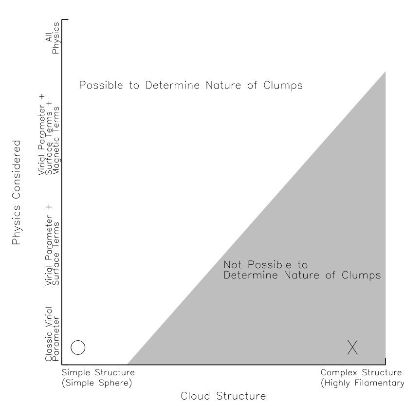
We have verified that for purely spherical cores that are completely isolated (i.e. not lying in the same line-of-sight from other cores) with distinct velocity profiles, the masses, sizes, and linewidths derived from the PPP and PPV cubes agree.333In the simulation, however, we found that relatively isolated structures give different best fit power laws from the PPP and synthetic observations. If such “simple” clouds exists, and given the discrepancy in derived power-laws between PPP and synthetic observations of the filamentary simulation we consider, we speculate that there should be some transition region in parameter space beyond which traditional analysis methods used to assess the “boundedness” of structures cannot be applicable. We illustrate this concept in Figure 7, which broadly indicates that consideration of more physical processes is necessary for accurately assessing the boundedness of more complex clouds.
For a very simple spherical clump, it may be possible to determine if the object is bound or not using the classical virial parameter analysis (however, see caveats expounded by Ballesteros-Paredes, 2006). Including additional physics may increase the accuracy of the analysis. It may not be possible to apply a given analysis, such as the straightforward virial parameter analysis, to more complex clouds, indicated by the shaded region in Figure 7. Accurately determining the bounded nature of objects within complex clouds would require the consideration of more physics, such as the surface terms in the virial analyses, and/or the effects of magnetic fields.
Figure 7 is only a schematic, intended to illustrate that considering more physics, rather than just kinetic and gravitational energies, is required for reliably determining the nature of the clumps in more complex clouds. The depiction of a distinct transition separating the structures for which it is possible to determine their bounded nature from those for which it is not is simply an arbitrary illustration. The confirmation of agreement in the masses, sizes, and linewidths of simple, isolated cores between the PPV and PPP cubes is representative of a situation residing near the origin in Figure 7 (marked by a circle). In this case a simple virial analysis would produce identical results between a PPP and PPV analysis, and thus may accurately reveal the dynamical state of the clumps. On the other hand, our analysis of the highly filamentary simulation (shown in Figure 1) clearly lies within the shaded regime of Figure 7 where the cloud structure is rather complex (marked by a cross). An investigation into the bounded nature of the clumps in this simulation would require consideration of more physics than those included in the classic virial analysis.
The parameter space depicted in Figure 7 does not indicate the level of modeling necessary to handle the effect of projection. In our analysis, we have simply represented the scale of the clumps as radii of circles with areas equal to that of the projected clump. The simulation we consider is rather filamentary, and so our method of assigning a “radius” to characterize the extent of the cloud may be partially responsible for the discrepancy in measured power-law correlations between the PPP and synthetic observation cases. As indicated, assuming spherical symmetry may be sufficient for spherical cores with certain density and velocity profiles. However, such idealized cores might not exist in nature, thus requiring better modeling efforts even for the most simple objects.
In our analysis, we have not considered effects of chemistry and/or radiative transfer. We simply consider a purely optically thin medium, within which radiation emerges from all matter, or regions with densities above a threshold density, and assume thermodynamic equilibrium. However, the ISM is comprised of various components at different temperatures (e.g Heiles & Troland, 2003); individual cold clouds may also be embedded in warmer gas (Hennebelle & Inutsuka, 2006). The physical state of molecular clouds may thus be more complex than that considered here. Further, the synthetic observations have insignificant noise levels. Even in excluding more complex physics and instrumental effects intrinsic to real observations, we still find rather significant differences between the measured properties of the cloud from the 3D simulation data compared with the synthetic observations. Thus, any discrepancies in the observed structure, from either a PPV cube or a column density map, from the 3D structure of the cloud can be fully attributed to the effect of geometric projection.
Though we have shown that projection may produce inaccurate scaling relations for a given observed cloud, comparing scaling relations between various observations may still prove to be worthwhile. For example, if analyses of PPV cubes, or 2D column density maps, of different molecular clouds produce different linewidth- and/or mass- size relationships, there may be some intrinsic physical process that could be responsible for the differences (e.g. Kauffmann et al. 2010b, in preparation). Some processes, such as heating and cooling, may play the most influential roles in sculpting one cloud, but may be insignificant compared to the effect of magnetic fields and gravity in another; thus, the (observed) scaling relations of those two clouds could be different.
To infer accurate cloud characteristics from the value of the exponents of the derived scaling relation, a thorough understanding of the effect of projection is a necessity. Analyses of various simulations could be an avenue toward such an understanding (Ballesteros-Paredes & Mac Low, 2002; Dib & Kim, 2007; Dib et al., 2007). In this work, we have only assessed one particular simulation. More analyses on different simulations, e.g. those with different magnetic field configurations, or including the effects of heating and cooling, should advance our understanding on how the “observed” mass- and linewidth- size scaling relations, and ultimately the virial parameter, varies through the combined effects of geometric projection and the different physical processes at work.
5 Summary
We assess the effect of geometric projection in deriving cloud properties, using a simulation of a molecular cloud. Using dendrograms (Rosolowsky et al., 2008), we identify contiguous structures in the 3D simulation dataset and idealized synthetic observations of the simulation. We measure the masses, sizes, and linewidths of structures in PPP and PPV cubes, as well as in column density maps of the simulated cloud. We subsequently perform a virial analysis to compare the bounded state of clumps in the simulation with that assessed from the synthetic observations. Our main results and conclusions are:
1) Identified clumps from the 2D column density map with large extents ( 0.8 pc) have masses in agreement with those obtained from 3D PPP cube. These large scale structures contain much of the total mass of the cloud. However, at smaller scales, the 2D clumps have systematically higher masses than those from the 3D simulation. The measured masses of these smaller scale clumps in the 2D map include contributions from all gas lying along the same lines of sight, resulting in inflated mass estimates.
2) Low mass structures with small extents ( 0.1 pc) identified in the PPV cube have similar masses to corresponding objects in the PPP data. However, many of these structures are not distinct objects in the PPP -cube; they are identified only because gas from different regions along (or near) the same line of sight happens to have similar line of sight velocities. Further, high spectral and spatial resolution would be required to identify those structures from spectral line observations. On the other hand, at large scales (R 0.1), PPV structures systematically have lower masses than PPP structures. This discrepancy again arises because of line of sight effects: a large scale structure in the PPP data might be identified as numerous lower mass structures in the PPV cube due to gradients in the line of sight velocity.
3) When only turbulent velocities are considered, the cumulative distribution of clumps from the 3D PPP data give different indices in the - and power law relationships compared to those from the 2D column density map and PPV cube of the simulated cloud. After including the contribution from thermal pressure, the linewidth has a lower limit at the value of . This results in similar best fit power-law indices from the PPP and PPV analyses, though there is a large degree of scatter. Further, the PPV clumps systematically have lower linewidths than those of the PPV clumps, often differing by a factor 2 (Figures 3-4 and Table 1).
4) Due to the differences in the measured properties from the PPP data and synthetic observations, there is a discrepancy in the identified scale beyond which the clumps are assessed to be bound. Despite the differences indicated by points 2) and 3), a virial analysis of the clumps in the PPP and PPV cubes show similar trends. But, we suggest that the similarity should not lead to the interpretation that a PPV analysis can accurately reveal the dynamical state of the observed clumps.
5) Taking 2) - 4) together, we conclude that projection effects can be rather significant, leading to inaccurate interpretations of the dynamical state of the cloud. We speculate that for a simple spherical cloud, the classic virial analysis, where the surface and magnetic terms are omitted (among other assumptions), may be sufficient for reliably determining whether cores are bound or not. We suggest that highly filamentary clouds require consideration of additional physics (Figure 7). We also remark that better modeling techniques are necessary to properly account for the effect of projection, as well as to appropriately handle the the non-spherical shapes of cloud structures.
References
- Adler & Roberts (1992) Adler, D. S. & Roberts, Jr., W. W. 1992, ApJ, 384, 95
- Ballesteros-Paredes (2006) Ballesteros-Paredes, J. 2006, MNRAS, 372, 443
- Ballesteros-Paredes & Mac Low (2002) Ballesteros-Paredes, J. & Mac Low, M.-M. 2002, ApJ, 570, 734
- Ballesteros-Paredes et al. (1999) Ballesteros-Paredes, J., Vázquez-Semadeni, E., & Scalo, J. 1999, ApJ, 515, 286
- Bertoldi & McKee (1992) Bertoldi, F. & McKee, C. F. 1992, ApJ, 395, 140
- Collins et al. (2010) Collins, D. C., Xu, H., Norman, M. L., Li, H., & Li, S. 2010, ApJS, 186, 308
- Dib & Kim (2007) Dib, S. & Kim, J. 2007, in Astronomical Society of the Pacific Conference Series, Vol. 365, SINS - Small Ionized and Neutral Structures in the Diffuse Interstellar Medium, ed. M. Haverkorn & W. M. Goss, 166–+
- Dib et al. (2007) Dib, S., Kim, J., Vázquez-Semadeni, E., Burkert, A., & Shadmehri, M. 2007, ApJ, 661, 262
- Falgarone et al. (1992) Falgarone, E., Puget, J., & Perault, M. 1992, A&A, 257, 715
- Gammie et al. (2003) Gammie, C. F., Lin, Y.-T., Stone, J. M., & Ostriker, E. C. 2003, ApJ, 592, 203
- Goodman et al. (2009) Goodman, A. A., Rosolowsky, E. W., Borkin, M. A., Foster, J. B., Halle, M., Kauffmann, J., & Pineda, J. E. 2009, Nature, 457, 63
- Heiles & Troland (2003) Heiles, C. & Troland, T. H. 2003, ApJ, 586, 1067
- Hennebelle & Inutsuka (2006) Hennebelle, P. & Inutsuka, S. 2006, ApJ, 647, 404
- Heyer et al. (2009) Heyer, M., Krawczyk, C., Duval, J., & Jackson, J. M. 2009, ApJ, 699, 1092
- Larson (1981) Larson, R. B. 1981, MNRAS, 194, 809
- Mac Low (1999) Mac Low, M.-M. 1999, ApJ, 524, 169
- McKee & Zweibel (1992) McKee, C. F. & Zweibel, E. G. 1992, ApJ, 399, 551
- Myers & Goodman (1988) Myers, P. C. & Goodman, A. A. 1988, ApJ, 329, 392
- Ostriker et al. (2001) Ostriker, E. C., Stone, J. M., & Gammie, C. F. 2001, ApJ, 546, 980
- Pichardo et al. (2000) Pichardo, B., Vázquez-Semadeni, E., Gazol, A., Passot, T., & Ballesteros-Paredes, J. 2000, ApJ, 532, 353
- Pineda et al. (2009) Pineda, J. E., Rosolowsky, E. W., & Goodman, A. A. 2009, ApJ, 699, L134
- Rosolowsky & Blitz (2005) Rosolowsky, E. & Blitz, L. 2005, ApJ, 623, 826
- Rosolowsky et al. (2008) Rosolowsky, E. W., Pineda, J. E., Kauffmann, J., & Goodman, A. A. 2008, ApJ, 679, 1338
- Solomon et al. (1987) Solomon, P. M., Rivolo, A. R., Barrett, J., & Yahil, A. 1987, ApJ, 319, 730
- Stutzki & Guesten (1990) Stutzki, J. & Guesten, R. 1990, ApJ, 356, 513
- Teuben (1995) Teuben, P. 1995, in ASP Conf. Ser. 77: Astronomical Data Analysis Software and Systems IV, ed. R. A. Shaw, H. E. Payne, & J. J. E. Hayes, 398–+
- Truelove et al. (1997) Truelove, J. K., Klein, R. I., McKee, C. F., Holliman, II, J. H., Howell, L. H., & Greenough, J. A. 1997, ApJ, 489, L179+
- Williams et al. (1994) Williams, J. P., de Geus, E. J., & Blitz, L. 1994, ApJ, 428, 693
| Power Law; index | PPPaa | PPVbb | Column Densitybb |
|---|---|---|---|
| ; | 3.03 0.02 | 2.56 0.01 | 1.95 0.03 |
| ; | 0.72 0.01 | - | - |
| ( pc); | 0.49 0.02 | - | - |
| ; | - | 0.85 0.01 | - |
| ( pc); | - | 0.82 0.01 | - |
| ; | 0.44 0.01 | 0.39 0.004 | - |
| ( pc); | 0.42 0.02 | 0.49 0.01 | - |
