A first principles explanation for the density limit in magnetized plasmas

Fusion research on magnetic confinement is confronted with a severe problem concerning the electron densities $n_{e}$ to be used in fusion devices. Indeed, high densities are mandatory for obtaining large efficiencies, whereas it is empirically found that catastrophic disruptive events occur for densities exceeding a maximal one $n_{e}^{M}$. On the other hand, despite the large theoretical work “there is no widely accepted, first principles model for the density limit” (see green2 , abstract). Here, we propose a simple microscopic model of a magnetized plasma suited for a tokamak, for which the existence of a density limit is proven. This property turns out to be a general collective feature of electrodynamics of point charges, which is lost in the continuum approximation. The law we find is

$$n_{e}^{M}=1.74\,\frac{1}{m_{e}c^{2}}\,\frac{B^{2}}{\mu_{0}}$$ (1)

where $\mu_{0}$ is the vacuum permeability, $c$ the speed of light, $m_{e}$ the electron mass, and $B$ the magnetic field. As shown in Fig. 1, the theoretical limit (big circles) is in rather good agreement with the empirical data, actually a surprisingly good one for a model based on first principles, with no adjustable parameter.

The way in which law (1) was established is an interesting example of an encounter between fundamental and applied research. Indeed three of the present authors are involved since some time in studies of a general character concerning the microscopic electrodynamics of systems of point particles (see cg and mcg ), in which both the mutual retarded forces, and the radiation reaction force of Abraham Lorentz and Dirac dirac (see also massimodirac and jackson ) are taken into account. One of the results obtained is the proof of an identity conceived by Wheeler and Feynman wf , and an appreciation of the role the latter plays in allowing for the very existence of a dispersion relation. In particular, some examples of dispersion relations were given (see cg , Fig. 1), which exhibit, as the matter density is increased, a bifurcation of a topological character, entailing an instability. But the physical relevance of this fact was not emphasized. Such a density controlled bifurcation impressed instead very much those of the present authors who deal with plasma physics, who suggested it may be relevant for fusion plasmas. To this end, the simplest possible model was formulated, that should capture, within the frame of the foundational works mentioned, the essential physics of a magnetized plasma, confined in a tokamak configuration (the most studied one for fusion plasmas). The model is presented here, together with the deduction of law (1). Preliminarily, the main evidence for the existence of a density limit in tokamaks is recalled, and it is discussed how well does law (1) fit the data.

For the purposes of the present paper, all is needed to know about tokamaks is essentially that they are toroidal devices in which the confining magnetic field $B$ is the vector sum of a strong toroidal field $B_{t}$ produced by a set of coils wound around a torus, and of a much smaller poloidal field $B_{p}$ generated by a toroidal plasma current $I_{p}$. A few more details will be mentioned later.

Figure 1: Greenwald plot for three tokamak devices (data extracted from green2 ). Dotted line is the empirical Greenwald limit (2). Big circles are the theoretical predictions (1) for the same devices.

The empirical data which show the existence of a density threshold beyond which tokamaks cannot operate, were collected by Greenwald green2 in a classical figure, the data of which are reported here in Fig.1. In the figure, the electron densities $n_{e}$ at which three different tokamak devices could actually be operated are reported versus the so-called Greenwald parameter $n_{G}\equiv I_{p}/\pi a^{2}$ (where $a$ is the minor radius of the torus), which is presumed to be the relevant control parameter. Indeed, the law proposed by Greenwald for the maximal density (dotted line in the figure) is

$$n_{e}^{M}=\alpha_{G}\,I_{p}/\pi a^{2}\ ,$$ (2)

where $\alpha_{G}$ is a constant with suitable dimensions, such that $\alpha_{G}=1$ in the units indicated in the figure. The theoretical predictions given by (1) are also reported as big circles.

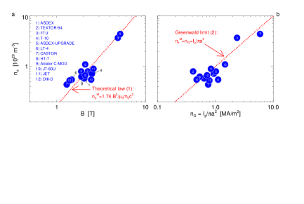
Figure 2: Density limit values for various conventional tokamak machines vs $B$ in a and vs $I_{p}/\pi a^{2}$ in b. Dotted line in a is the proposed theoretical law (1), and in b is the empirical law (2). For the various devices the points given are representative of disruptive events actually due to an increase of density or of an operative condition declared to be close to a density limit (see references Stabler ; DeVries ; Frigione ; Merezhkin ; Merthens ; Howard ; Dyabilin ; Asif ; Bombard ; Takenaga ; Saibene ; Petrie ).

Thus there naturally arises the question, how is it possible that two analytically different predictions, (1) and (2), happen to agree with each other, at least in a few definite cases. The reason is that one has

$$\frac{B}{\mu_{0}}\approx\,b\,\frac{I_{p}}{\pi a^{2}}\ ,\quad b\,=\,q(a)\,R\,\frac{1}{\kappa^{1/2}(1+\kappa^{2})}\ ,$$ (3)

where the dimensional coefficient $b$ (a length) is not a universal one, but depends parametrically on geometric factors and operative conditions characterising each experiment. These are the major and the minor radii $R$ and $a$, the plasma elongation $\kappa$ (equal to 1 for circular plasmas, see Miyamoto pg. 277), and the edge safety factor $q(a)$ defined below.

This is seen as follows. One has $B_{p}=\mu_{0}I_{p}/(2\pi a\kappa^{1/2})$. Furthermore, in the approximation $B\approx B_{t}$, one has $B\approx(B_{t}/B_{p})B_{p}$, while the operative parameter $B_{t}/B_{p}$ is determined by the edge safety factor $q(a)$ which, for the simplified case of an elliptical plasma (see Miyamoto ), is defined as $q(a)=(a/R)(B_{t}/B_{p})(1+\kappa^{2})\,/2$. This gives relation (3). The formula for $b$ in the general case is also easily established.

Now, magnetohydrodynamic stability requires $q(a)>2$, but the actual value at which each experimental data point of Fig. 1 was taken is not given in the literature. So we assumed $q(a)=4$, which is a typical operational value, and this introduces an uncertainty in the theoretical points reported in Fig. 1.

Thus, we decided to look directly at the experimental values available in the literature, from which a definite estimate of $B$ could be obtained, and this we did for conventional tokamaks more recent than those in Fig. 1. Such values are plotted in Fig. 2, where they are compared to laws (1) and (2). The agreement with law (1) is perhaps a little better.

This fact might have relevant implications for future tokamaks, as it implies a favorable density scaling for machines with large values of the product $R\,B$. For example, let us consider the international thermonuclear experimental reactor (ITER) Iter , which should operate at a toroidal field of 5.3 T. According to law (1) it would be able to operate at densities up to $n_{e}^{M}=4.7\times 10^{20}m^{-3}$. This is a value more than three times larger than that expected according to Greenwald law (2) for a plasma current of 15 MA, which is the corresponding value of $I_{p}$ for a $q(a)=3$ scenario.

It is worth mentioning that a $B^{2}$ dependence of the density limit in the ALCATOR C experiment was noted in the past by Granetz Granetz , although such a clear dependence was not observed on other experiments (see for example Petrie for the DIII-D tokamak). Also, one should point out that tokamaks with very low aspect ratio $R/a$ (spherical tokamaks) and reversed field pinches (RFP) Lorenzini , for which the validity of the Greenwald scaling has been proposed Valisa , seem not to fit well into the proposed $B^{2}$ scaling. This, perhaps, suggests that at low magnetic fields other effects, not considered in the present simple model, might come into play.

We show now how law (1) was obtained, in the frame of microscopic electrodynamics of point particles (see cg and mcg ), rather than of magnetohydrodynamics (see for example gold , chapter 17), or of the mean field theories of the Vlasov approach. We describe the plasma as constituted of point particles obeying Newton equations, with both the retarded electromagnetic interactions among all particles and the radiation reaction force taken into account. We then concentrate on the role played by the gyration of the electrons around the magnetic field lines, and so ignore their motions along the field lines, and also ignore the electrostatic part of the problem. Finally we also limit ourselves to the extremely simplified case of a one–dimensional array.

So we introduce the following model. Given a constant magnetic field $B$, which we take oriented along the ${z}$ axis of a cartesian coordinate system, we constrain each electron, say the $n$-th one, to move on a plane parallel to the ($x,y$) plane, so that its $z_{n}$ coordinate is fixed. The simplest choice is to take $z_{n}=nl$, with $n\in Z$, for a given positive step $l$. Each electron, say the $n$–th one, is subjected to the external magnetic field $B$, and also to the electromagnetic field created by the electrons themselves. Namely, the sum of the Liénard–Wiechert fields, which are determined as the retarded solutions of Maxwell equations having as sources the charge and the current densities of each other electron $m\neq n$, and the Abraham–Lorentz–Dirac radiation reaction force, due to the motion of the $n$–th electron itself, The latter is given, in the nonrelativistic approximation, by $(2/3)e^{2}/(4\pi\epsilon_{0}c^{3})\,{\hskip 2.0pt\ddot{\hbox{}}\hskip 2.5pt\dot{\hbox{}}\kern-5.0pt{\mathbf{x}}}_{n}$, where $e$ is the electron charge and ${\mathbf{x}}_{n}$ the position vector of the electron.

We then perform the dipole approximation. Thus we neglect the magnetic field due to the $m$–th electron, and for the electric field created by it we take the well known expression for a dipole. Finally, we approximate the distance between electrons $n$ and $m$ by $r_{n,m}=l|n-m|$. The system of equations of motion defining the model is then

$$\begin{split}{\ddot{x}}_{n}-\omega_{c}{\dot{y}}_{n}-\frac{2}{3}\,\frac{e^{2}}{4\pi\epsilon_{0}m_{e}c^{3}}\,{{\hskip 2.0pt\ddot{\hbox{}}\hskip 2.5pt\dot{\hbox{}}\kern-5.0pt{x}}}_{n}&=-\frac{e^{2}}{4\pi\epsilon_{0}m_{e}}\sum_{m\neq n}\Big{[}\frac{x_{m}(t-r_{nm}/c)}{r^{3}_{nm}}+\frac{1}{c}\frac{{\dot{x}}_{m}(t-r_{nm}/c)}{r^{2}_{nm}}+\frac{1}{c^{2}}\frac{{\ddot{x}}_{m}(t-r_{nm}/c)}{r_{nm}}\Big{]}\\ {\ddot{y}}_{n}+\omega_{c}{\dot{x}}_{n}-\frac{2}{3}\,\frac{e^{2}}{4\pi\epsilon_{0}m_{e}c^{3}}\,{{\hskip 2.0pt\ddot{\hbox{}}\hskip 2.5pt\dot{\hbox{}}\kern-5.0pt{y}}}_{n}&=-\frac{e^{2}}{4\pi\epsilon_{0}m_{e}}\sum_{m\neq n}\Big{[}\frac{y_{m}(t-r_{nm}/c)}{r^{3}_{nm}}+\frac{1}{c}\frac{{\dot{y}}_{m}(t-r_{nm}/c)}{r^{2}_{nm}}+\frac{1}{c^{2}}\frac{{\ddot{y}}_{m}(t-r_{nm}/c)}{r_{nm}}\Big{]}\\ \end{split}$$ (4)

for $n\in Z$, where $\epsilon_{0}$ is the vacuum permittivity, and $\omega_{c}=eB/m_{e}$ the Larmor or cyclotron frequency of the electrons in the external magnetic field $B$. This is an infinite system of linear equations with delay, which is just a simple variant of the system considered in cg .

Our aim is now to investigate the stability properties of the system, as the control parameters $n_{e}=1/l^{3}$ and $B$ (or equivalently $\omega_{c}$) are varied. Following a completely standard procedure (see for example chandra ), we compute the normal modes of the system and determine the values of the parameters for which the frequencies become complex. So we look for normal mode solutions with wavenumber $k$ and angular frequency $\omega$, i.e., of the form

$$x_{j}=A_{x}e^{i(klj+\omega t)}\ ,\quad y_{j}=A_{y}e^{i(klj+\omega t)}\ .$$ (5)

This leads to a linear system in the unknowns $A_{x}$, $A_{y}$, from which the dispersion relation between $\omega$ and $k$ is found by equating the determinant to zero. This gives two real equations in the two unknowns $\omega$ and $k$, namely,

$$\Big{(}\frac{\omega}{\omega_{c}}\Big{)}^{2}\pm\,\frac{\omega}{\omega_{c}}\ +p\,F(kl,l\omega/c)=0,\quad p=\frac{\omega_{p}^{2}}{\omega_{c}^{2}}\ .$$ (6)

$$\frac{2}{3}\,\frac{e^{2}}{4\pi\epsilon_{0}m_{e}c^{3}}\,\omega^{3}-G(kl,l\omega/c)=0\ .$$ (7)

Here, $\omega_{p}$ is the familiar plasma frequency defined by

$$\omega_{p}^{2}=e^{2}/\epsilon_{0}m_{e}l^{3}\ =n_{e}\,e^{2}/\epsilon_{0}m_{e}\ ,$$ (8)

while $F$ and $G$, as functions of the variables $\alpha=kl$, $\beta=l\omega/c$, are defined by

$$\begin{split}F(\alpha,\beta)&=\frac{1}{4\pi}\Big{[}\beta^{2}\log\big{(}2\,|\cos\beta-\cos\alpha|\,\big{)}-f(\alpha,\beta)\Big{]}\\ G(\alpha,\beta)&=\beta^{3}-g(\alpha,\beta)\ ,\end{split}$$

the functions $f$ and $g$ being the ones already introduced in cg , namely,

$$\begin{split}f(\alpha,\beta)=\sum_{n\neq 0}(\frac{\cos(n\alpha-|n|\beta)}{|n^{3}|}-\beta\frac{\sin(n\alpha-|n|\beta)}{|n^{2}|})\\ g(\alpha,\beta)=\sum_{n\neq 0}(\frac{\sin(n\alpha-|n|\beta)}{|n^{3}|}+\beta\frac{\cos(n\alpha-|n|\beta)}{|n^{2}|})\ .\end{split}$$

Some details concerning the summation of the series leading to the term $\beta^{2}\log\big{(}2\,|\cos\beta-\cos\alpha|\big{)}$ entering the function $F$ are here omitted.

Now, one meets here with a deep question of principle. Indeed, for fixed values of the parameters $l$ and $\omega_{c}$ one has two equations in two unknowns ($\omega$ and $k$), and this would not allow for the existence of a dispersion relation, i.e., of a function $\omega=\omega(k)$ for a continuous range of values of $k$. However, the existence of a dispersion relation is guaranteed by the fact that equation (7) actually is an identity. In fact, this is a particular case of a general identity, conceived by Wheeler and Feynman wf and first proven in cg (see section 6) for a one-dimensional case and in mcg for a three-dimensional one.

So, the problem of obtaining the dispersion relation is reduced to solving (6) in the unknown $\omega=\omega(k)$, in which $p=\omega_{p}^{2}/\omega_{c}^{2}$ plays the role of a parameter. In Fig. 3 the dispersion relations are shown for a cyclotron frequency $\omega_{c}=3.8\cdot 10^{11}Hz$, and for several values of the parameter $p=\omega_{p}^{2}/\omega_{c}^{2}$ (or of the corresponding electron density $n_{e}/n_{G}$, normalized to the Greenwald density $n_{G}\equiv I_{p}/\pi a^{2}$).

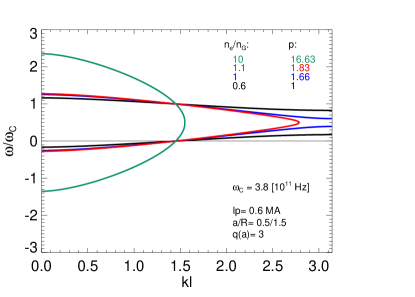
Figure 3: The dispersion curves, solutions of equation (6) (with the plus sign), in the plane ($kl$, $\omega/\omega_{c}$) for $\omega_{c}=3.8\times 10^{11}$ Hz, and for several values of the parameter $p=\omega_{p}^{2}/\omega_{c}^{2}$ (or equivalently of the electron density $n_{e}$, normalized to the empirical $n_{G}$ limit).

The most important qualitative result is that normal modes are found to exist (for all $k$) only below a critical value of $p$, i.e., below a certain threshold of plasma density. Indeed, starting up from low densities, at a certain critical density a bifurcation is seen to occur, characterized by the fact that the curves no more intersect the vertical axis $kl=\pi$. This means that for values of $k$ just below $\pi/l$ equation (6) does not admit a real solution, so that the corresponding frequencies acquire an imaginary part, and the whole system becomes unstable. Numerical computations not reported here show that the characteristic time of the instability is of the order of $2\pi/\omega_{c}$ and that above the critical density the Wheeler and Feynman identity is no more satisfied.

Notice that this phenomenon of the existence of a maximal allowed density is obviously lost if one introduces the continuum approximation, i.e., is a characteristic feature of the discrete structure of matter. Indeed, following mcg , the continuum approximation corresponds to deal with wavelengths much larger than the step $l$, i.e., to assume $k\ll\pi/l$, whereas the existence of a density limit depends on the behavior of the system for $kl\simeq\pi$.

We have now to determine the bifurcation value of the parameter $p$. As the bifurcation occurs for $kl=\pi$ and for values of $\omega/\omega_{c}\leq 1$, i.e., for $l\omega/c\simeq 0$, one can just limit oneself to study equation (6) for a fixed value of the function $F$, namely $F(\pi,0)$, so that one is simply reduced to deal with an algebraic equation of second degree. One computes $F(\pi,0)\simeq 0.14$, and so real values of $\omega$ are found to exist only for $p\lesssim 1.74$. This, together with the definition of $p$ in (6) and $\epsilon_{0}\mu_{0}=1/c^{2}$, gives law (1).

Notice that law (1) has the same form of the Brillouin limit Brillouin , which is known to apply to the case of nonneutral plasmas Davidson . The main difference with respect to our procedure is that in the case of the Brillouin limit the electric field acting on each electron is introduced within a mean field approach, whereas here it is computed in the frame of a many–body microscopic theory. Correspondingly, we find that the instability involves normal modes with wavelengths of the order of the mean electron distance, so that it escapes a mean field approach. In particular, such an instability is found to occur in neutral plasmas, for which the mean charge density vanishes, and the Brillouin approach cannot be used.

A final comment concerns the possibility of dealing with the other main magnetic configuration studied for the confinement of fusion-relevant plasmas, i.e., the Stellarator Boozer . The present model does not directly apply. Indeed, in the Stellarator a large amount of power is typically transferred to the electrons through electron cyclotron resonance heating (ECRH), and this requires to add in our model a forcing term.

In conclusion, through an extremely simplified model of a magnetized plasma suited for a tokamak, based on first principles, we have proved the existence of a density limit, beyond which the system becomes unstable. The law thus found differs from the usually accepted one, and this fact might have relevant implications for future tokamaks.

The authors wish to thank Dr. Nicola Vianello for fruitful discussions.
This work, supported by the European Communities under the contract of Association between EURATOM/ENEA, was carried out within the framework the European Fusion Development Agreement.

References

- (1) Greenwald, M., Density limits in toroidal plasmas, Plasma Phys. Control. Fusion 44, R27–R80 (2002).
- (2) Carati, A. and Galgani, L., Nonradiating normal modes in a classical many-body model of matter-radiation interaction, Nuovo Cim. 118 B, 839-849 (2003).
- (3) Marino, M., Carati, A, Galgani, L., Classical Light dispersion theory in a regular lattice, Annals of Physics 322, 799-823 (2007).
- (4) Dirac, P.A.M., Classical Theory of Radiating Electrons, Proc. Royal Soc. London 167, 148–169 (1938).
- (5) Marino, M., Classical electrodynamics of point charges, Annals of Physics 301, 85–127 (2002).
- (6) Jackson, J.D.,Classical Electrodynamics, New York, J. Wiley and Sons (1975).
- (7) Wheeler, J.A. and Feynman, R.P., Interaction with the absorber as the mechanism of radiation, Rev. Mod. Phys. 17, 157-181 (1945).
- (8) Miyamoto, K., Plasma Physics and Controlled Nuclear Fusion, Berlin, Springer (2005).
- (9) Stabler, Ä. et al., Density limit investigations on ASDEX, Nucl. Fusion 32, 1557 (1992).
- (10) de Vries, P.C., Rapp, J., Schüller, F.C. and Tokar, M.Z., Influence of recycling on the density limit in TEXTOR-94, Phys. Rev. Lett. 80, 3519-3522 (1998).
- (11) Frigione, D. et al., High density operation on Frascati Tokamak Upgrade, Nucl. Fusion 36, 1489 (1999).
- (12) Merezhkin, V.G., Electron energy balance near the density limit in T-10 and FTU OH regimes, 33rd EPS Conference on Plasma Phys., Rome, 19-23 June 2006 ECA Vol. 30I, P-4.085 (2006).
- (13) Merthens, V. et al., High density operation close to Greenwald limit and H Mode limit in ASDEX UPGRADE, Nucl. Fusion 37, 1607-1614 (1997).
- (14) Howard, J. and Person, M., Cold bubble formation during tokamak density limit disruptions, Nucl. Fusion 32, 361-377 (1992).
- (15) Dyabilin, K. S. et al., Global energy balance and density limit on CASTOR tokamak, Czech. J. Phys. B 37, 713-724 (1987).
- (16) Asif, M. et al, Study of recycling and density limit in the HT-7 superconducting tokamak, Phys. Lett. A 336, 61-65 (2005).
- (17) LaBombard, B. et al., Particle transport in the scrape-off layer and its relationship to discharge density limit in Alcator C-MOD, Phys. Plasmas 8, 2107-2117 (2001).
- (18) Takenaga, H. et al., Compatibility of advanced tokamak plasma with high density and high radiation loss operation in JT-60U, Nucl. Fusion 45, 1618-1627 (2005).
- (19) Saibene, G. et al., The influence of isotope mass, edge magnetic shear and input power on high density ELMy H modes in JET, Nucl. Fusion 39, 1133-1156 (1999).
- (20) Petrie, T.W., Kellman, A.G. and Mahdavi, M.Ali, Plasma density limits during ohmic L mode and elming H Mode operation in DIII-D, Nucl. Fusion 33, 929-952 (1993).
- (21) The ITER physics basis, Nucl. Fusion 47, S1-S413 (2007).
- (22) Granetz, R.S., Density threshold for magnetohydrodynamic activity in Alcator C, Phys. Rev. Lett. 49, 658-661 (1982).
- (23) Lorenzini, R. et al, Self-organized helical equilibria as a new paradigm for ohmically heated fusion plasmas, Nature Phys. 5, 570-574 (2009).
- (24) Valisa, M. et al., The Greenwald density limit in the Reversed Field Pinch, IAEA-CN-116/EX/P4-13, 20th IAEA Fusion Energy Conference, 1-6 November 2004, Vilamoura, Portugal.
- (25) Goldston, R.J. and Rutherford, P.H., Introduction to Plasma Physics, Bristol, IOP Publishing (1995).
- (26) Chandrasekhar, S., Hydrodynamic and Hydromagnetic Stability, Oxford, Clarendon Press (1961).
- (27) Brillouin, L., A theorem of Larmor and its importance for electrons in magnetic fields, Phys. Rev. 67, 260-266 (1945).
- (28) Davidson, R.C., Physics of Nonneutral Plasmas, Redwood City, Addison–Wesley (1990).
- (29) Boozer, A.H., What is a stellarator?, Phys. Plasmas 5, 1647-1655 (1998).