The level crossing and inverse statistic analysis of German stock market index (DAX) and daily oil price time series
F. Shayeganfar,a M. Hlling,b J. Peinke,b and M. Reza Rahimi Tabara,c
aDepartment of Physics, Sharif University of Technology,
P.O.Box 11365-9161, Tehran 11365, Iran
bCarl von Ossietzky University, Institute of Physics, D-26111
Oldenburg, Germany
c Fachbereich Physik, Universität Osnabrück,
Barbarastraße 7, 49076 Osnabrück, Germany
The level crossing and inverse statistics analysis of DAX and oil
price time series are given. We determine the average frequency of
positive-slope crossings, , where is the average waiting time for observing the
level again.
We estimate the probability , which provides us the probability of
observing times of the level with positive slope, in
time scale . For analyzed time series we found that
maximum is about . We show that by using the level
crossing analysis one can estimate how the DAX and oil time series
will develop. We carry out same analysis for the increments of DAX
and oil price log-returns,(which is known as inverse statistics)
and provide the distribution of waiting times to observe some level for the increments.
PACS: 05.45.Tp, 02.50.Fz.
1 Introduction
Stochastic processes occur in many natural and man-made phenomena, ranging from various indicators of economic activities in the stock market, velocity fluctuations in turbulent flows and heartbeat dynamics, etc [1]. The level crossing analysis of stochastic processes has been introduced by (Rice, 1944, 1945) [2-26], and used to describe the turbulence [16], rough surfaces [27], stock markets [28], Burgers turbulence and Kardar-Parisi-Zhang equation [29, 30]. The level crossing analysis of the data set has the advantage that it gives important global properties of the time series and do not need the scaling feature. The almost of the methods in time series analysis are using the scaling features of time series, and their applications are restricted to the time series with scaling properties. Our goal with the level crossing analysis is to characterize the statistical properties of the data set with the hope to better understand the underlying stochastic dynamics and provide a possible tool to estimate its dynamics. The level crossing and inverse statistics analysis can be viewed as the complementary method to the other well-known methods such as, detrended fluctuation analysis (DFA) [31], detrended moving average (DMA) [32], wavelet transform modulus maxima (WTMM) [33], rescaled range analysis (R/S) [34], scaled windowed variance (SWV) [35], Langevin dynamics [36], detrended cross-correlation analysis [37], multifactor analysis of multiscaling [38], etc.
We start with formalism of the level crossing analysis. Consider a time series of length given by (here is the log-return of DAX and oil prices). The log-return is defined as , where is the price at time . Let denote the averaged number of slope crossing of in time scale with (we set also the average to be zero). The averaged can be written as , where is the average frequency of positive slope crossing of the level . The positive level crossing has specific importance that it gives the next average time scale that the price will be greater than the again up to specific level. For narrow band processes it has been shown that the frequency can be deduced from the underlying joint probability distributions function (PDF) for and . Rice proved that [2]
| (1) |
where is the joint PDF of and . For discrete time series (of course all of real data are discrete) the frequency can be written in terms of joint cumulative probability distribution, as [39],
| (2) | |||||
| (3) |
where is the joint PDF of and . The inverse of frequency gives the average time scale that one should wait to observe the given level again.
The rest of this paper is organized as follows: Section 2 is devoted to summary of level cross analyzing of DAX and daily oil price log-returns. The inverse statistics of DAX and Oil price time series are given in section 3. Section 4 closes with a discussion and conclusion of the present results.
2 level crossing
Here, at first we provide the results of level crossing analysis for two normalized log-return time series, daily German stock market index (the DAX) and daily oil price. The daily fluctuations in the oil price and DAX time series were belong to the period 1998-2009. We also study the asymmetric properties of level crossing analysis for positive and negative level crossing of the time series. To have a comparison we provide also level crossing analysis of synthesized uncorrelated noise. Also we will provide the results of level crossing analysis of high frequency data for DAX with sample rate (1/min), where we have used data points and belongs to the period 1994-2003.
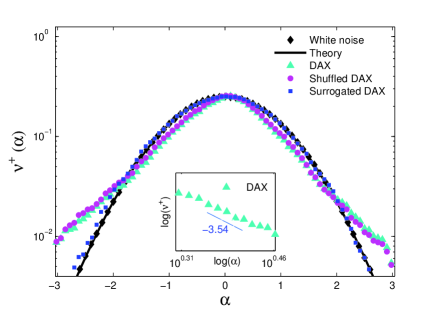
Figure 1 shows the frequency for daily log-returns of DAX and synthesized uncorrelated noise. The PDF of synthesized uncorrelated noise is Gaussian and it has white noise nature (i.e. its correlation has delta-function behavior). As shown in figure 1, their level crossing frequency are almost similar near to and have deviation for levels in the tails. The difference is related to the non-Gaussian PDF of DAX log-return time series (see below). For the normalized Gaussian uncorrelated noise one can show that the frequency is given by
| (4) |
where is the error function. In figure 1 a comparison between the analytical and numerical results for uncorrelated Gaussian time series is given. For Gaussian uncorrelated data the frequency behaves as:
| (5) | |||||
| (6) |
while we have found that for daily DAX and oil price time series have power-law tails with exponents and , respectively (see inset of figure 1). It means that the DAX and oil price time series have non-Gaussian tails for their level crossing. We note that within the error bars, the exponent . However the exponent may depends on the sample rate of data acquisition (see below). The exponent can be estimated using the method proposed in [51, 52, 53]. If the PDF or follow a power law with exponent , one can estimate the power-law exponent by sorting the normalized returns or levels by their sizes, , with the result [52] , where (N - 1) is the number of tail data points.
In general, there are two reasons to have non-Gaussian tails for level crossing of given time series; (i) due to the fatness of the probability density function (PDF) of the time series, in comparison to a Gaussian PDF. By definition a fat PDF is defined via the behavior of its tails. If its tail goes to the zero slower than a Gaussian PDF then we call it as fat tail PDF. In this case, non-Gaussian tails cannot be changed by shuffling the series, because the correlations in the data set are affected by the shuffling, while the PDF of the series is invariant, (ii) due to the long-range correlation in time series. In this case, the data may have a PDF with finite moments, e.g., a Gaussian distribution. The easiest way to distinguish whether the PDF shape or long-range correlation is responsible for the fastnesses of for the DAX and oil log-returns time series, is by analyzing the corresponding shuffled and surrogate time series. The level crossing analysis will be sensitive to correlation when the time series is shuffled and to probability density functions (PDF) with fat tails when the time series is surrogated. The long range correlations are destroyed by the shuffling procedure and in the surrogate method the phase of the discrete Fourier transform coefficients of time series are replaced with a set of pseudo-independent distributed uniform quantities. The correlations in the surrogate series do not change, but the probability function changes to Gaussian distribution [40, 41, 42].
In figure 1 the level crossing frequency of shuffled and surrogated DAX time series are given. The figure shows that the frequency has more difference for original and surrogated time series and means that the non-Gaussian tails for due to the fatness of PDF is dominant [16]. We have found similar results for daily oil price log-returns.
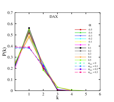
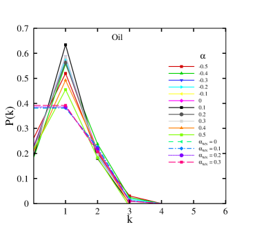
Now let us introduce the PDF, , which provides us the probability of observing times of the level with positive slope, in the averaged time scale . By construction the average , i.e. will be unity and satisfies the normalization condition . In principle we can assume that the upper bound, i.e. to be infinity. For the processes and levels that satisfy , we expect to have a good estimation about the future of process. This means that one will observe the level with high probability in time scale at least once. For the levels that the PDF satisfies , the process will be not predictable. Figure 2 shows the PDF , for daily DAX and oil price log-return time series for different levels . We plotted also for some levels of synthesized Gaussian uncorrelated data to have a comparison. As shown in figure 2 the upper bound is about 6, which means that it is almost impossible to observe same level in average time scale more than 6 times, even for the white noise. We used data points for white noise synthesized data and found that the maximum number of observing is also about 6.
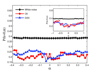
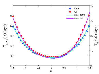
To find the best interval for the estimation of time series future, we consider the variation of the PDF, with respect to the level . This will enable us to find the range and intervals of levels that one can estimate the future of these time series with high accuracy. In figure 3 the PDFs for daily DAX, oil and uncorrelated synthesized time series, are given. It shows that the of daily DAX and oil time series for the interval has smaller probability with respect to uncorrelated time series. It means that with high probability (with respect to white noise), one can observe the level at least once in time scale for s belong to this interval. The typical time scale for these interval is about 4 days for the daily DAX and oil time series, respectively. The corresponding time scales for different s are shown in figure 4. For the daily DAX and oil price time series (for the interval ) we found the following empirical curve fittings:
| (7) | |||||
| (8) |
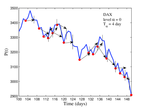
where ‘s have the dimension ”days”. To check the applicability level crossing for forecast of the time series, in figure 5 we plotted the daily time series of DAX and indicates the points with level with red points. The average for this level indicated by vertical lines. We expect that in this time scale one should observe another red points with high probability. We also investigated the asymmetry properties of time series with respect to positive and negative slops.
Finally, we have done similar analysis to the high frequency DAX time series and find that the best interval to estimate the future is . The typical time scale belong to this levels is about sec and the obtained exponent was . For this time series, the averaged time scale depends on the level as:
| (9) |
where has dimension in seconds.
3 Inverse statistics
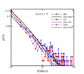
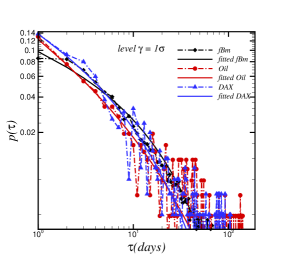
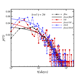
To the modeling the statistical properties of financial time series Simonsen, et al. [43] asked the ”inverse” question: what is the smallest time interval needed for an asset to cross a fixed return level ? or what is the typical time span needed to generate a fluctuation or a movement in the price of a given size [42-46]? The inverse statistics is the distribution of waiting times needed to achieve a predefined level of return obtained from every time series. This distribution typically goes through a maximum at a time so called the optimal investment horizon, which is the most likely waiting time for obtaining a given return [48]. Let be the price at time . The logarithmic return calculated over the interval is, . Given a fixed log-returned barrier, , of an index, the corresponding time span is estimated for which the log-return of index for the first time reaches the level . This can also be called the first passage time through the level for . In figure 6, we plotted the probability distribution of normalized waiting time needed to reach return levels for daily oil, daily DAX log-returns and integrated white noise data (i.e. fractional Brownian motion fBm).
As figures 6 show, for the zero level for , inverse statistics of the two markets does not deviate from fractional Brownian motion while they are rather different behavior from fBm for and . We fit the waiting times distribution functions for different level via the Weibull distribution function [54]:
| (10) |
Where is the stretched exponent (or shape parameter) and is the characteristic time scale. We found and for fBm and Oil and DAX time series and summarized results in Table 1.
TABLE I. The stretched exponent and characteristic time scale fitted by Weibull distribution for various time series.
| 0 | fBm | 0.423 | 1.849 |
|---|---|---|---|
| 0 | Oil | 0.347 | 1.132 |
| 0 | DAX | 0.312 | 5.791 |
| 1 | fBm | 0.704 | 13.145 |
| 1 | Oil | 0.496 | 7.943 |
| 1 | DAX | 0.600 | 6.836 |
| 2 | fBm | 0.956 | 34.178 |
| 2 | Oil | 0.878 | 32.480 |
| 2 | DAX | 0.988 | 18.631 |
4 Conclusion
In summary, we analyzed the DAX and oil daily price log-return time series using the level crossing method and find the average waiting time for observing the level again. This is a similar analysis as what has been done in Refs. [49, 50, 51]. They have been carried out the level crossing of the volatility time series, instead of the time series itself. We define and estimate the probability of observing K times of the level , in time scale . We show that by using the level crossing analysis one can estimate the future of the daily DAX and oil time series with good precision for the levels in the interval . Also, using the inverse statistics we estimate the waiting time probability distribution for two financial markets, i.e. oil and DAX time series.
References
- [1] R. Mantegna and H.E. Stanley, An Introduction to Econophysics: Correlations and Complexities in Finance (Cambridge University Press, New York, 2000); R. Friedrich, J. Peinke and M. Reza Rahimi Tabar, ”Importance of Fluctuations: Complexity in the View of Stochastic Processes” Encyclopedia of Complexity and Systems Science, 3574 (Springer, Berlin 2009).
- [2] S. O. Rice, Bell System Tech. J. 23 282 (1944); ibid. 24 46 (1945).
- [3] W. Liepmann, Helv. Phys. Acta 22, 119 (1949); H. W. Liepmann and M. S. Robinson, NACA TN, 3037 (1952).
- [4] H. Steinberg, P.M. Schultheiss, C. A.Wogrin and F. Zwieg, J. Appl. Phys. 26 195 (1955).
- [5] J. A. McFadden, IEEE Trans. Inform. Theory IT-2 146 (1956); IT-4 14 (1958).
- [6] C. W. Helstrom, IEEE Trans. Inform. Theory IT-3 232 (1957).
- [7] I. Miller and J. E. Freund, J. Appl. Phys. 27 1290 (1958).
- [8] A. J. Rainal, IEEE Trans. Inform. Theory IT-8, 372 (1962).
- [9] D. Slepian, Proc. Sympos. Time Series Analysis, Brown Univ., ed. M. Rosenblatt, Wiley, 1963, pp. 104 115.
- [10] K. Ito, J. Math. Kyoto Univ. 3 (1963/1964) 207 216.
- [11] S. M. Cobb, IEEE Trans. Inform. Theory IT-11 220 (1965).
- [12] N. D. Ylvisarer, Annals of Math. Statist. 36 1043 (1965).
- [13] M. R. Leadbetter and J. D. Cryer, Bull. Amer. Math. Soc. 71 561 (1965); R. N. Miroshin, St. Petersburg Univ. Math. 34 30 (2001).
- [14] Orey, Z. Wahrscheinlichkeitstheor. Verwandte Geb. 15, 249 (1970)
- [15] J. Abrahams, IEEE Trans. Inform. Theory IT-28 677 (1982).
- [16] K. R. Sreenivasan, A. Prabhu, and R. Narasimha, J. Fluid Mech. 137, 251 (1983); K. R. Sreenivasan, Annu. Rev. Fluid Mech. 23, 539 (1991).
- [17] A. J. Rainal, IEEE Trans. Inform. Theory 34 1383 (1988); A. J. Rainal, IEEE Trans. Inform. Theory 36 1179 (1990).
- [18] J. T. Barnett and B. Kedem, IEEE Trans. Inform. Theory 37 1188 (1991); G. L. Wise, ibib bf 38 213 (1992).
- [19] I. Rychlik, Extremes 3 331 (2000).
- [20] J. Davila and J. C. Vassilicos, Phys. Rev. Lett. 91, 144501 (2003).
- [21] St. Lück, Ch. Renner, J. Peinke and R. Friedrich, Physics Letters A359 335 (2006).
- [22] D. Hurst and J. C. Vassilicos, Phys. Fluids 19, 035103 (2007).
- [23] N. Mazellier and J. C. Vassilicos, Phys. Fluids 20, 015101 (2008).
- [24] Poggi D, Katul, BOUNDARY-LAYER METEOROLOGY 136 219 (2010).
- [25] M. F. Kratz and J. R. Le n, Extremes 13 315 (2010).
- [26] N. Rimbert, Phys. Rev. E 81 056315 (2010).
- [27] F. Shahbazi, S. Sobhanian, M. R. Rahimi Tabar, S. Khorram, G. R. Frootan, and H. Zahed, J. Phys. A36, 2517 (2003).
- [28] G. R. Jafari, M. S. Movahed, S. M. Fazeli, M. R. Rahimi Tabar, and S. F. Masoudi, J. Stat. Mech., P06008 (2006).
- [29] A. Bahraminasab, H. Rezazadeh, A. A. Masoudi, J. Phys. A: Math. Gen. 39, 3903 3909 (2006).
- [30] A. Bahraminasab M. S. Movahed , S. D. Nasiri , A. A. Masoudi, M. Sahimi, Journal of Statistical Physics 124 (6): 1471-1490, (2006)
- [31] C.-K. Peng, J. Mietus, J. M. Hausdorff, S. Havlin, H. E. Stanley, and A. L. Goldberger, Phys. Rev. Lett. 70, 1343(1993).
- [32] E. Alessio, A. Carbone, G. Castelli, and V. Frappietro, Eur. Phys. J. B 27, 197 (2002).
- [33] J. F. Muzy, E. Bacry, and A. Arneodo, Phys. Rev. Lett. 67, 3515 (1991).
- [34] H. E. Hurst, R. P. Black, and Y. M. Simaika, Long-Term Storage. An Experimental Study (Constable, London, 1965).
- [35] A. Eke, P. Herman, L. Kocsis, and L. R. Kozak, Physiol. Meas. 23, R1-R38 (2002).
- [36] R. Friedrich and J. Peinke, Phys. Rev. Lett. 78, 863 (1997); G.R. Jafari, S.M. Fazlei, F. Ghasemi, S.M. Vaez Allaei, M. R. Rahimi Tabar, A. Iraji Zad, and G. Kavei, Phys. Rev. Lett. 91, 226101 (2003); F. Ghasemi, J. Peinke, M. Sahimi and M. Reza Rahimi Tabar, Eur. Phys. J. B 47, 411 (2005); P. Sangpour, G. R. Jafari, O. Akhavan, A. Z. Moshfegh and M. Reza Rahimi Tabar, Phys. Rev. B71 155423 (2005); F. Ghasemi, M. Sahimi, J. Peinke and M. Reza Rahimi Tabar, J. Biological Physics 32 117 (2006); G. R. Jafari, M. Sahimi, M. Reza Rasaei and M. Reza Rahimi Tabar, Phys. Rev. E 83, 026309 (2011); F. Shayeganfar, S. Jabbari-Farouji, M. S. Movahed, G. R. Jafari and M. Reza Rahimi Tabar, Phys. Rev. E 81, 061404 (2010); A. Farahzadi, P. Niyamakom, M. Beigmohammadi, N. Mayer, M. Heuken, F. Ghasemi, M. Reza Rahimi Tabar, T. Michely and M. Wuttig, Europhysics Letters 90, 10008 (2010); S. Kimiagar, M. S. Movahed, S. Khorram and M. Reza Rahimi Tabar, Journal of Statistical Physics 143 148 167 (2011).
- [37] B. Podobnik and H. E. Stanley, Phys. Rev. Lett 100, 084102 (2008).
- [38] F. Wang, K. Yamasaki, S. Havlin, and H. E. Stanley, Phys. Rev. E 79, 016103 (2009).
- [39] F. Ghasemi, M. Sahimi, J. Peinke, R. Friedrich, G. R. Jafari, and M. Reza Rahimi Tabar, Phys. Rev. E 75, 060102R (2007)
- [40] J. Theiler and D. Prichard, Fields Inst. Commun. 11,99 (1997).
- [41] T. Schreiber and A. Schmitz, Physica D 142, 346 (2000).
- [42] B. Podobnik, D.F. Fu, H.E. Stanley and P.Ch. Ivanov, Eur. Phys. J. B 56, 47 (2007).
- [43] I. Simonsen, M.H. Jensen, and A. Johansen, Eur. Phys. J. B, 27 (2002).
- [44] M.H. Jensen, Phys. Rev. Lett 83, 76 (1999).
- [45] L. Bifarele, M. Cencini, D. Vergni, A. Vulpiani, Eur. Phys. J. B bf 20, 473 (2001).
- [46] S. Karlin, A First Course in Stochastic Processes (Academic Press, New York, 1966).
- [47] M. Ding, G.Rangarajan, Phys. Rev. E 52, 207 (1995).
- [48] H. Ebadi, M. Bolgorian and G. R. Jafari, Physica A 389 5530 (2010).
- [49] K. Yamasaki, L. Muchnik, S. Havlin, A. Bunde, and H. E. Stanley, Proc. Natl. Acad. Sci. USA 102, 9424 (2005).
- [50] F. Wang, K. Yamasaki, S. Havlin, and H. E. Stanley, Phys. Rev. E 73, 026117 (2006).
- [51] B. Podobnik, D. Horvatic, A. Peterson, H. E. Stanley, Proc. Natl. Acad. Sci. USA 106, 22079 (2009).
- [52] B. M. Hill, A simple general approach to inference about the tail of a distribution. Ann Stat 3, 1163 (1975).
- [53] A. Pagan, The econometrics of financial markets. J Empirical Finance 3, 15 (1996).
- [54] P. C. Ivanov, A. Yuen, B. Podobnik and Y. Lee, Phys. Rev. E 69, 056107 (2004). Captions FIG. 1. The level crossing analysis of the DAX log-returns (original, shuffled and surrogated) and uncorrelated Gaussian time series. Inset: the log-log plot of level crossing frequency vs level for DAX log-return time series. The Gaussian uncorrelated time series has exponential tails (), while the daily DAX time series has power-low tails with exponent . FIG. 2. The PDf vs for different levels for normalized log-returns time series of the daily German stock market index (DAX) (top), oil daily price (bottom) and uncorrelated synthesized data. FIG. 3. The PDF vs for DAX, oil daily price and uncorrelated synthesized normalized log-return time series. The inset is same figure with wide range of ‘s. The results for uncorrelated synthesized data are plotted to have a comparison. FIG. 4. The level dependence of average time for daily DAX and oil price log-return time series. FIG. 5. The points (red) with level for daily DAX time series. We expect that in this time scale one should observe another red points with high probability. FIG. 6. The probability distribution of normalized waiting time needed to reach return levels at scale , i.e. , and for two financial markets including oil and DAX time series. Solid curves are the fitted curve (Weibul distribution) based on Eq. (7).