Analytical continuation of imaginary axis data using maximum entropy
Abstract
We study the maximum entropy (MaxEnt) approach for analytical continuation of spectral data from imaginary times to real frequencies. The total error is divided in a statistical error, due to the noise in the input data, and a systematic error, due to deviations of the default function, used in the MaxEnt approach, from the exact spectrum. We find that the MaxEnt approach in its classical formulation can lead to a nonoptimal balance between the two types of errors, leading to an unnecessary large statistical error. The statistical error can be reduced by splitting up the data in several batches, performing a MaxEnt calculation for each batch and averaging. This can outweigh an increase in the systematic error resulting from this approach. The output from the MaxEnt result can be used as a default function for a new MaxEnt calculation. Such iterations often lead to worse results due to an increase in the statistical error. By splitting up the data in batches, the statistical error is reduced and and the increase resulting from iterations can be outweighed by a decrease in the systematic error. Finally we consider a linearized version to obtain a better understanding of the method.
I Introduction
The analytical continuation of spectral functions from imaginary time to real energies is a difficult problem due to its ill-posed nature, i.e., the output can depend very sensitively on the input. For strongly correlated electrons, however, this is an important problem. Most approaches for such systems involve uncontrolled approximations. Using quantum Monte-Carlo (QMC) methods or quantum cluster methods it is, however, possible to obtain accurate data for Green’s functions and response functions on the imaginary axis, raising the problem of analytical continuation to the real axis. Since these methods provide data with statistical noise, the ill-posed nature of the problem makes analytical continuation very difficult.
This problem can be treated within the Bayesian theory.Jarrell ; MEMref The problem is regularized by introducing an entropy in terms of the deviation of the output real axis spectrum from some default function. The importance of the entropy is controlled by a parameter , which is determined using statistical arguments.Jarrell ; MEMref This method is referred to as the Maximum Entropy (MaxEnt) method. It has been rather successful in performing analytical continuations. Alternative methods have been proposed, such as Padé approximations,Vidberg ; Baker singular value decomposition,svd stochastic regularizationRubtsov and sampling schemes.Mishchenko ; Kiamars
In this paper we focus on the MaxEnt method. This method is usually discussed in terms of the Bayesian theory. Here we start from the equations generated by the MaxEnt formalism and use an algebraic approach to analyze the theory. We discuss the accuracy that can be obtained within this framework. The error in the output spectral function can be split up in a statistical error, due to the noise in the input data, and a systematic error, due to the deviation of the default function from the true spectrum. The choice of determines the relative size of these errors. In the classical MaxEnt method the most probable is chosen.Jarrell We find that this choice can make the statistical error unnecessary large.
The input data is typically given as a number of samples, , where each sample gives a (noisy) version of the imaginary time function . We find that the accuracy can sometimes be improved by splitting up the samples in sub sets (batches), with samples in each batch. We then perform MaxEnt calculations, each with samples, and then average the results, instead of performing one MaxEnt calculation samples. This approach reduces the statistical error at the cost of an increase in the systematic error.
We also discuss the possibility of an iterative MaxEnt method, where the output is used to define a new default function. This usually works poorly, and we show that this is due to an increase in the statistical error, overwhelming the improvement in the systematic error. However, if the data are split in batches, as discussed above, the importance of the statistical error can be reduced to the point where the approach improves the total accuracy.
To further analyze the results, we introduce an alternative method with a new, slightly different definition of the entropy. This leads to a set of linear equations, where the propagation of the errors can be analyzed more easily and features of the MaxEnt method better understood. This method, however, does not guarantee a positive spectral function, and it is less useful for practical calculations.
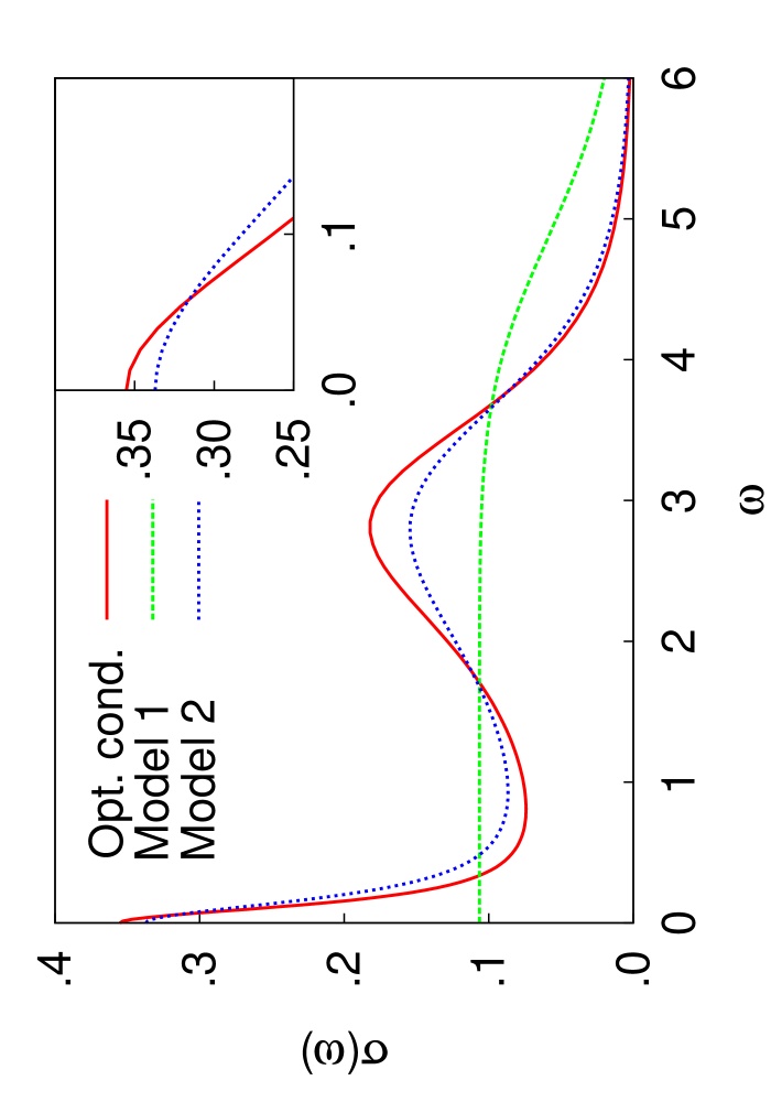
In this paper we focus on a response function, the optical conductivity . We introduce a typical , which in the following will be refered to as the “exact” . The form of was chosen using results for the two-dimensional Hubbard model as a guide. This model of can easily and accurately be transformed to imaginary axis data. We add statistical noise to the data and then transform the data back to the real axis, using the various modifications of the MaxEnt method. If a given method worked perfectly the that we started with should be recovered exactly. The deviations from the “exact” are then a measure of the accuracy of the different approaches.
As an example, Fig. 1 shows an “exact” optical conductivity and two default models used in the MaxEnt approach. The optical conductivity has a Drude like peak at and a “Hubbard” peak at corresponding to transitions between the Hubbard bands. The default models are chosen so that they satisfy the exact sum rule. The two models are chosen according to two different strategies. It is sometimes argued that the default model should contain little information, apart from certain exact results, such as sum rules. This way the results are not prejudiced by possible incorrect assumptions. Model 1 has been chosen this way. Alternatively, as a default model one can use the output from a calculation at a higher temperature . Model 2 has therefore been chosen to be quite similar to the “exact” result, but with all features somewhat broader. Model 2 will naturally deliver much more accurate output spectra.
The paper is organized as follows. In Sec. II we introduce the formalism. Sec. III describes how a MaxEnt calculation is performed as an average of several MaxEnt calculations and Sec. IV discusses an iterative MaxEnt method. In Sec. V we present a simplified entropy definition, leading to linear equations.
II Formalism
We introduce the basic formalism, essentially following Jarrell and Gubernatis,Jarrell and then provide error estimates. The function for imaginary time is related to a spectral function on the real frequency axis ,
| (1) |
via a kernel , given for some discrete values of . For the case of the optical conductivity, considered here, the kernel is given by
| (2) |
where is a weight factor chosen so that Eq. (1) corresponds to an integral over . For the electron Green’s function the corresponding kernel is
| (3) |
We introduce a likelihood function
| (4) |
where are data obtained from, e.g., a Monte-Carlo calculation, with the statistical accuracy , and has been calculated from Eq (1). We also introduce the entropy
| (5) |
where is a default model. The quantity is then minimized with respect . This leads to the equations
| (6) |
These equations are solved to obtain the spectral function . The quantity can be determined using statistical methods, giving the most probable . This is referred to as the classical MaxEnt method.Jarrell Alternatively, one can average the spectrum calculated for different values of , using the probability of that as a weighting function.Jarrell This method, Bryan’s method, gives similar results for the cases considered here.
To estimate the error in this approach, we express the calculated spectral function in terms of the exact result as
| (7) |
where is the error in . We assume that the error is sufficiently small that the logarithm in Eq. (6) can be expanded to lowest order. Then
| (8) |
where and is the error in due to the statistical noise. To solve these equations, we define
| (9) |
| (10) |
Using matrix notations,
| (11) |
The error is defined as
| (12) |
where denotes the average over many different realizations of the noise in the input data. Here is the error due to this noise and is the error due to the deviation
| (13) |
of the default function from the exact result. Since the noise is random, there is no contribution from the cross term in the square of the two terms in Eq. (11). The statistical error can then be written as
| (14) | |||||
The second equality was obtained by noticing that the terms do not contribute on the average and that the average of is . Later we consider the average over MaxEnt calculations, each using data with the statistical accuracy . The statistical error is then reduced by a factor of , since refers to the square of the error in the output spectrum.
For the systematic error we obtain
| (15) |
The results in Eqs. (14, 15) apply to the case when MaxEnt calculation is not iterated. For an iterative calculation we use Eq. (IV) below.
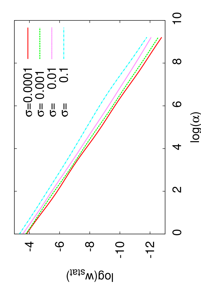
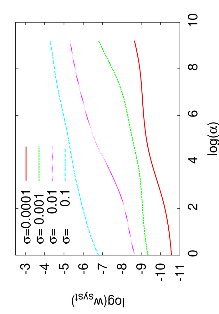
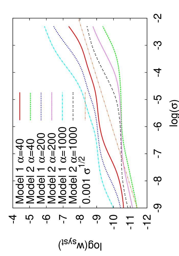
Fig. 2 shows and as a function of for different . The figure illustrates that behaves approximately as . This illustrates the importance of introducing entropy, i.e., using an . For , the matrix is ill-behaved and the statistical error would be huge. Since depends only weakly on , it is not possible to make small for by simply reducing (within reasonable limits). Introducing regularizes and leads to a manageable statistical error. The systematic error increases with and there is therefore an optimal value of where the total error is minimum. The dependence of the systematic error on is shown in Fig. 3. It behaves roughly as . The optimal therefore increases as is reduced. It also increases as the default model is made more accurate, e.g., by replacing default model 1 by model 2.
Since is often of particular interest we use a logarithmic -mesh. For the case we use
| (16) |
where . A small value of leads to a smaller spacing of the points close to . We have typically used points, , , and . For simplicity, we assume that the statistical error is given by
| (17) |
in terms of some overall accuracy . To perform these calculations we have developed a MaxEnt code, which was found to give almost identical results to a code made available to us by Jarrell.Jarrell
III Multiple MaxEnt calculations
A QMC calculation is arranged so that it gives a number of samples, , of . From these data one can calculate the statistical accuracy , check if the data are Gaussian and check for (undesirable) correlations between the noise for different values of .Jarrell The data are then averaged over to obtain that is the input for the MaxEnt calculation, possibly after removing correlations between the noise at different -points.Jarrell
We now consider the case where we have 100 samples, each with the accuracy . After averaging over all the samples, the accuracy of the resulting data is . The value of in a classical MaxEnt calculation depends on the specific realization of the noise. We therefore perform many calculations, each with a different realization of the noise, and average over . For , and , classical MaxEnt calculations using the spectrum in Fig. 1 and the default model 1 then gave on the average .
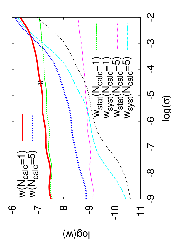
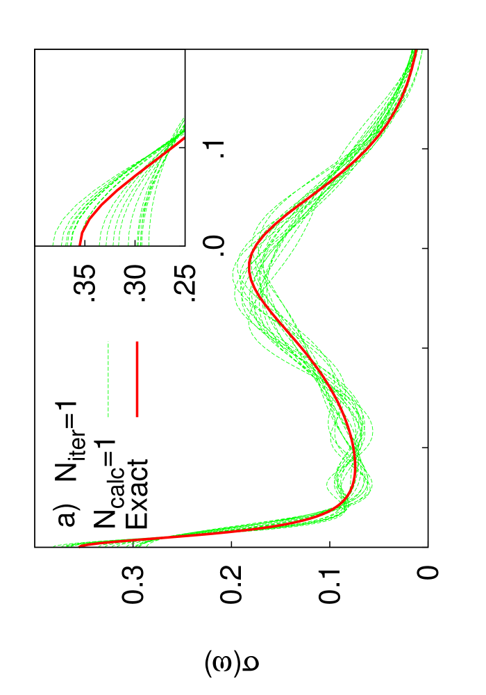
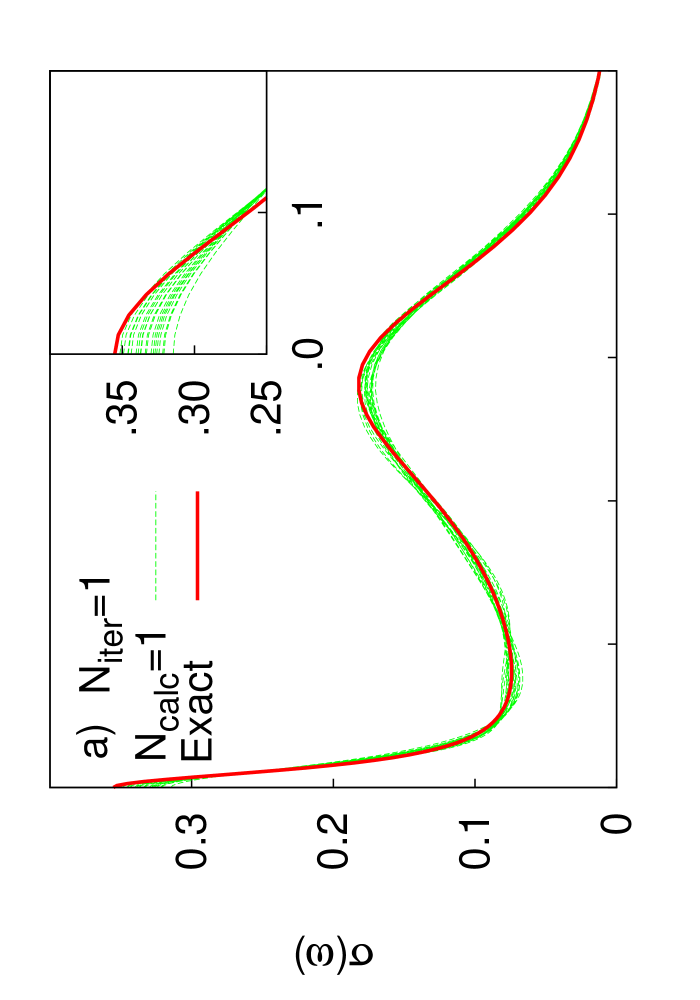
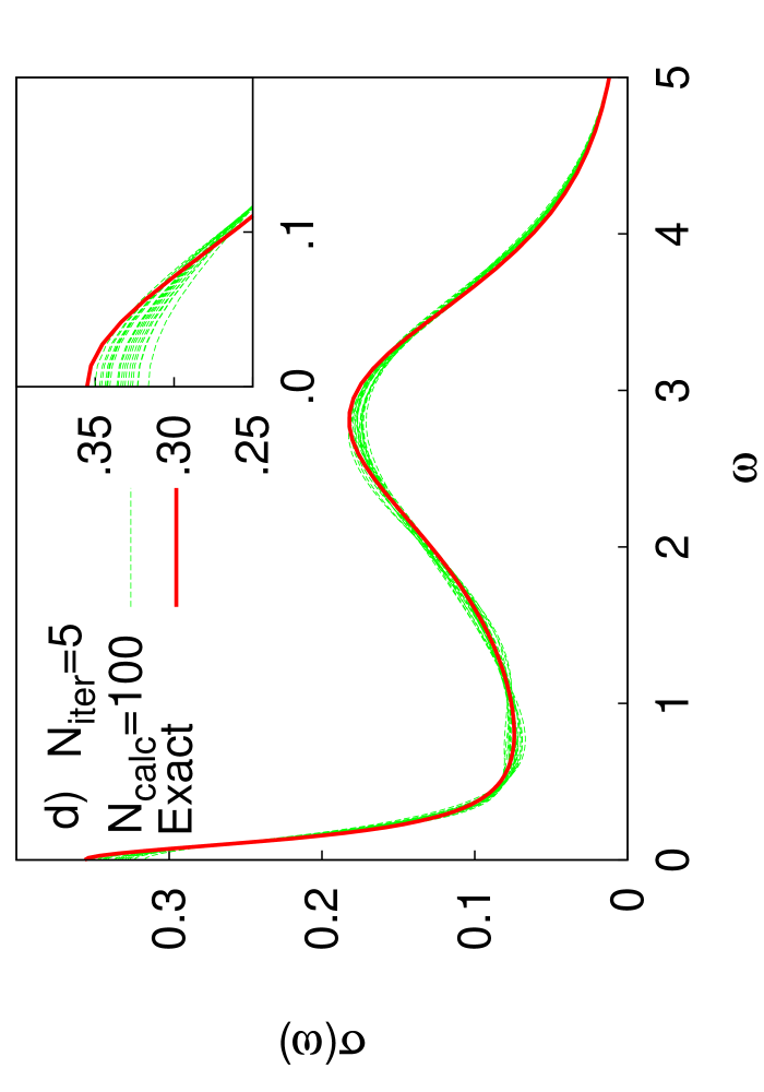
Fig. 4 shows the statistical and systematic errors for a fixed as a function of (). The cross gives the total error of a classical MaxEnt calculation corresponding to 100 samples with . The figure illustrates that the statistical error is much larger than the systematic error for the MaxEnt calculation. This is also illustrated in Fig. 5a. This shows the result of 20 MaxEnt calculations with different realizations of the noise, each with 100 samples with the accuracy . The thick (red) line shows the exact spectrum. The calculated spectra (thin green lines) scatter strongly around the exact result, illustrating a large statistical error. On the average, these spectra also deviate somewhat from the exact result, the value of being slightly too small and the Hubbard peak being somewhat shifted towards lower energies, illustrating a small systematic error.
| Default model | ||||||
|---|---|---|---|---|---|---|
| 1 | 40 | 1 | 1 | 6.7 10-4 | 1.4 10-4 | 8.1 10-4 |
| 1 | 40 | 5 | 1 | 1.4 10-4 | 2.1 10-4 | 3.5 10-4 |
| 1 | 40 | 1 | 2 | 14 10-4 | 1.3 10-4 | 15 10-4 |
| 1 | 40 | 100 | 4 | 0.4 10-4 | 0.9 10-4 | 1.3 10-4 |
| 2 | 720 | 1 | 1 | 4.2 10-5 | 4.4 10-5 | 8.6 10-5 |
| 2 | 720 | 2 | 1 | 2.3 10-5 | 5.6 10-5 | 7.9 10-5 |
| 2 | 720 | 1 | 2 | 9.7 10-5 | 3.3 10-5 | 13 10-5 |
| 2 | 720 | 20 | 8 | 2.4 10-5 | 3.9 10-5 | 6.3 10-5 |
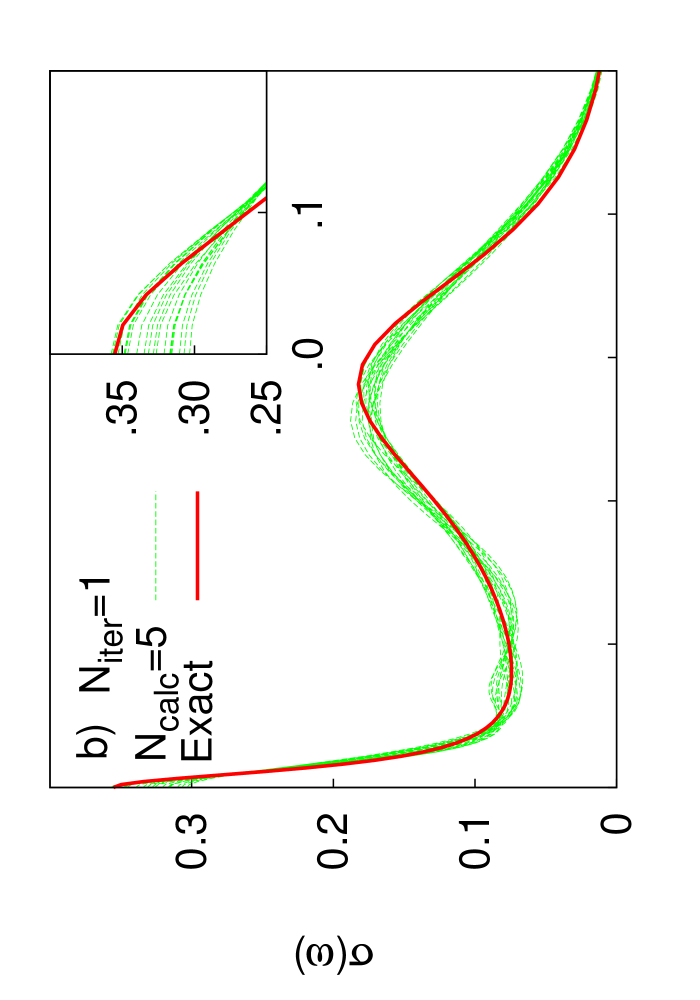
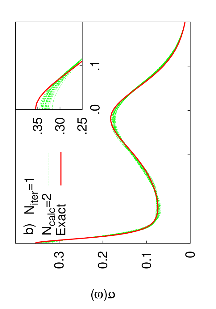
We next group the 100 samples in batches, each with 20 samples, and perform MaxEnt calculations. The accuracy of the data in these MaxEnt calculations is then only . This increases both the systematic and statistical errors somewhat. Averaging these calculation, however, reduces the statistical error by a factor . In Fig. 4 this leads to a large net reduction in the statistical error, which more than compensates for the increase of the systematic error. This is illustrated in Fig. 5b, which shows 20 such results, each one obtained by averaging MaxEnt calculations with samples, but with different realizations of the noise. The spread between the curves is substantially smaller ( vs. 0.00067) than in Fig. 5a, while the systematic error is somewhat larger ( vs. 0.00014). This leads to a substantial improvement in the total error ( vs. 0.00081). These results are also shown in Table 1.
The reason for this improvement is that that in the MaxEnt calculation with and that and have different dependencies on . For , Eq. (14) gives that . Splitting up the calculation in calculations makes the effective a factor larger, while averaging reduces the error by a factor . The net result would be an unchanged statistical error. It is therefore crucial that the method has been regularized by introducing an entropy. Fig. 4 shows that for realistic values of , actually has a quite weak dependence on , rather than behaving as . Splitting up the samples in several batches, and thereby reducing the accuracy of each batch, leads to a small increase in for each individual calculation. The averaging over calculations, however, reduces by a factor . At the same time is increased, but only by approximately a factor , since this quantity behaves approximately as and increases by a factor .
Fig. 6 and Table 1 show the corresponding results using default model 2. In this case the classical MaxEnt calculation chooses a value of that makes and comparable. The gain from splitting up the samples and performing several MaxEnt calculations is then much smaller.
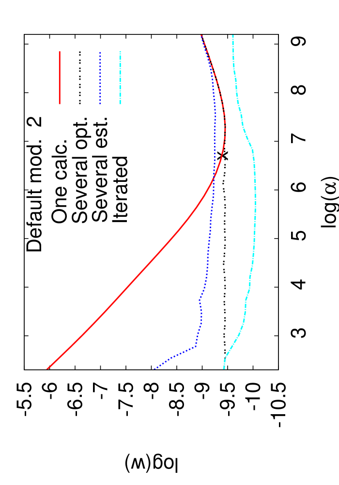
We are now in the position to discuss the limits of accuracy that can be obtained in this approach. We consider as before 100 samples with the accuracy and allow for any combination of , and . Starting from default model 1, we obtain the results shown in Fig. 7a. The curve “One calc.” shows the result of a traditional MaxEnt calculation, using all the samples in one calculation ( and ). If a classical MaxEnt calculation is performed, is obtained. This result is shown by a cross. We can see that this value of is not optimal, and a larger would have given a smaller error. We next allow for calculations, each using samples. We find the value of which gives the best agreement with the “exact” . This (“Several opt.”) leads to a much higher accuracy for small values of . The curve is almost flat as a function of over a substantial range. For large values of , gives the best accuracy, and the curve falls on top of the curve “One calc.”.
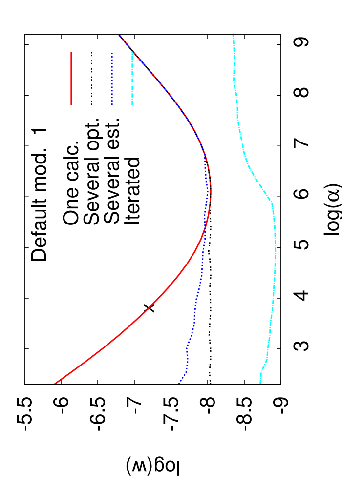
To provide a criterion for how to split up the data in batches, we consider the statistical error [(Eq. 14)] again. As before we consider the case of samples, each with the accuracy , divided in batches with samples in each. We define the product
| (18) |
where also depends on . The statistical error of the th calculation is then written as
| (19) |
where is the error in the th sample, and the statistical accuracy enters due to the averaging over samples. We then average over the calculations and obtain the error
| (20) |
The average difference between two calculations with and batches can then be written as
| (21) | |||
This result represents an average over many different realizations of the error . In addition to the statistical contribution to the difference there is a systematic contribution due to the error in the default function. We then compare calculations with and batches. In the second calculation the statistical error is larger and the systematic error is smaller. If the total difference between the two calculations is larger than twice the expected statistical difference, this suggests that the gain in the systematic error outweighs the loss in the statistical error and the second calculation is accepted. We then compare this calculation with a calculation with batches and if the latter is favorable the procedure is continued, considering , and batches. The resulting accuracy is shown by the curves “Several est.” in Fig. 7. This curve is above the curve “Several opt.”, but the difference is not very large for most values of .
IV Iterating MaxEnt
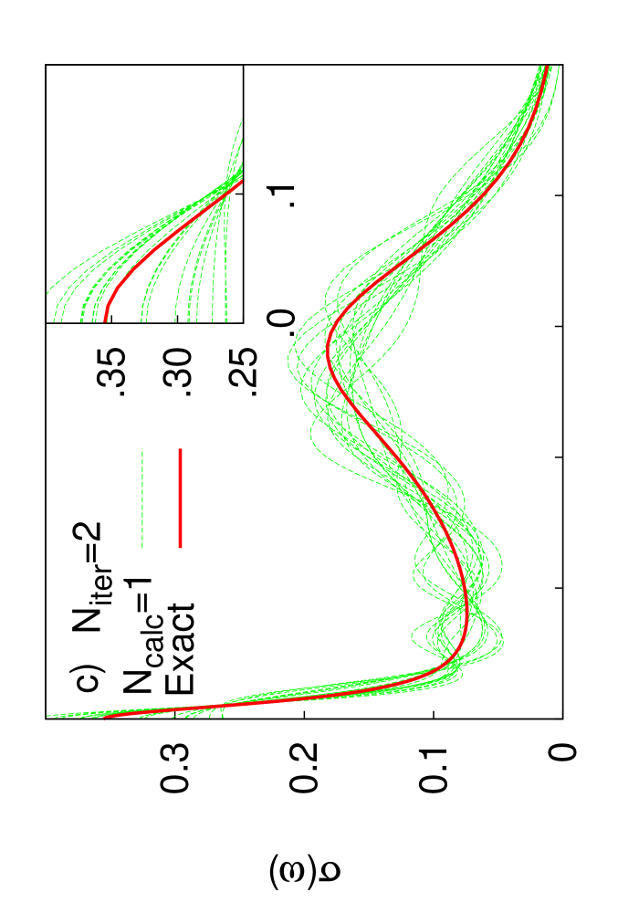
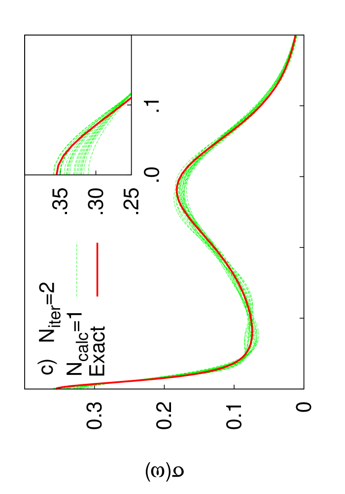
Once a MaxEnt calculation has been performed, one can try to improve the default function by using the output spectral function as a new default function. Such an iterative approach, however, is usually not recommended. Fig. 5c shows the results of such calculations using default model 1. Indeed, the spread between between different calculations is larger than in the noniterated case in Fig. 5a, implying an increased statistical error.
Eqs. (14, 15) used to calculate the statistical and systematic errors for a noniterated default model are not appropriate in the case of iterations. The reason is that the default model in this case contains statistical errors due to the iteration procedure. Instead we perform many calculations of the type shown in Fig. 5c, giving spectral functions , . We then calculate
| (22) | |||
Due to nonlinearity, some of the statistical error actually shows up as a systematic error in Eq. (IV), but this is neglected in the following.
The results in Table 1, shows that the statistical error is more than doubled after one iteration, while the systematic error is not correspondingly reduced.
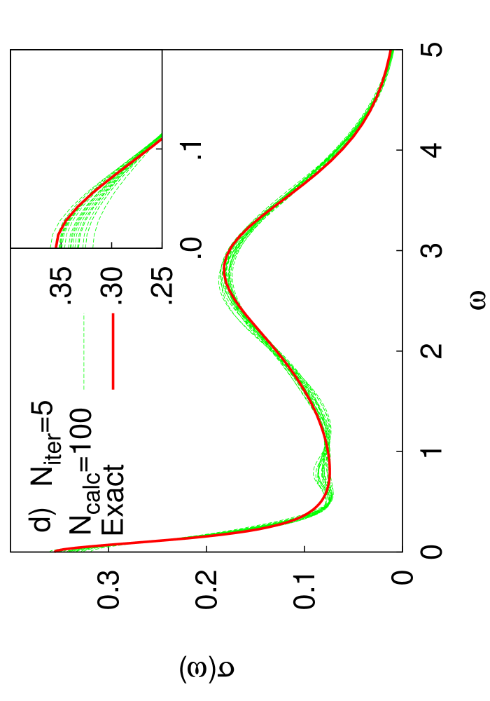
We next consider the case when the samples are split up in batches and default model 1 is used. Using and the total error is reduced, as is illustrated in Fig. 5d and Table 1. By using , we drastically reduce the statistical error. The following iterations increase the statistical error by a substantial factor, but it nevertheless remains small. At the same time the iterations reduce the systematic error, so that both are improved compared with the noniterated case. Fig. 6d shows similar results using default model 2. Since this model is very close to the exact result, iterations now lead to a small improvement, but even with such an accurate default function there is an improvement. In Fig. 7, the curve “Iterated” shows results when iteration is allowed (). This leads to a substantial improvement in the accuracy. Fig. 7b shows similar results for default model 2.
V Quadratic entropy
In Eq. (6) in Sec. II we introduced the entropy, containing a logarithm. As a result, the basic equations of MaxEnt are nonlinear, which makes the analysis complicated. For this reason, we introduce a new definition of the entropy, which is used in this section for analyzing the behavior of MaxEnt. The expression in Eq. (5) is expanded to lowest (second) order in the deviation between the solution and the default function. We then define this as the entropy, and use it in this section. This is then not an approximation but simply a new method. This method has some problems. For instance, it is not guaranteed that the spectrum is positive. Therefore we do not recommend the use of this method for calculating spectra, but simply use it to analyze MaxEnt.
We define the entropy
| (23) |
where we have allowed for the possibility of the MaxEnt calculation being iterated, i.e., depends on the iteration . The original default function is . This leads to the equations
| (24) | |||
where matrix notations have been used and and are diagonal matrices. Then . The error in is
| (25) |
where . We define
| (26) | |||
and a similar definition for as for . contains the same integration factor as has been used earlier, but due to the factor it gives more weight to errors where is small. We have
| (27) |
We find the eigenvalues and eigenvectors of the symmetric matrix . Introducing the expansion in these eigenvectors, we obtain
| (28) |
The matrix can be rewritten as
| (29) |
For the cases we have considered, the first matrix inside the bracket has a broad range of positive eigenvalues, extending from eigenvalues much smaller than one to much larger than one. As a result, the matrix is found to have some very small eigenvalues and many eigenvalues very close to one. This is illustrated in Table 2, which shows the lowest eigenvalues for the default model 1 and .
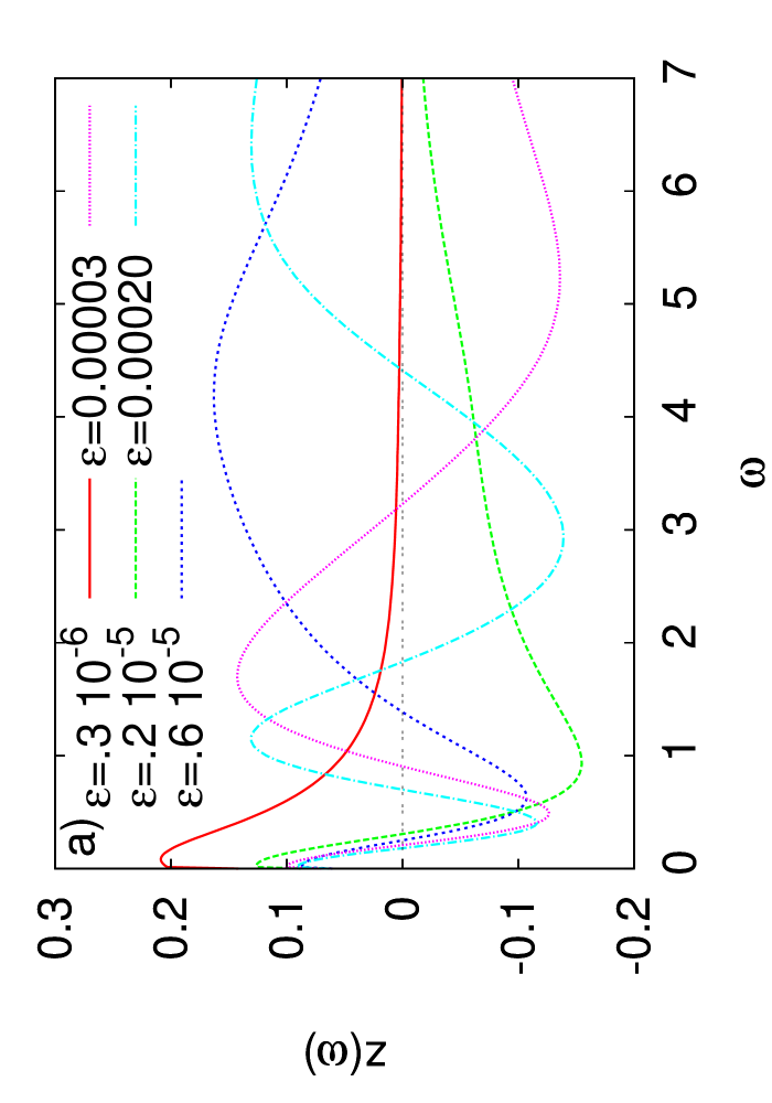
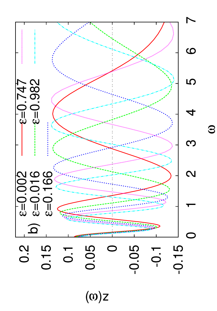
Fig. 8 shows the eigenfunctions corresponding to the lowest eigenvalues in Table 1. The lowest function is nodeless, and the higher functions have an increasing number of nodes. Functions with the eigenvalue very close to one oscillate so rapidly that the corresponding components of and tend to have small weights, as shown in Table 2. As a comparison, Table 2 also shows the expansion coefficients of the default model 2 in the eigenfunctions obtained for the default model 1 and .
It is crucial for the success of a MaxEnt calculation that the coefficients and are typically small for close to one. From Eq. (28) it follows that errors and corresponding to eigenvalues much smaller than one give a strongly reduced contribution to the error , while errors corresponding to the eigenvalue one are not reduced at all. For these components the deviation of the default model from the true result are taken over completely.
At the same time this sets the limits for MaxEnt calculations. A MaxEnt calculation fails if has structures on such a small energy scale that there are important expansion coefficients corresponding to eigenvalues close to one, since the MaxEnt calculation gives no additional information about these components. This also shows the danger of putting in too much structure on a small energy scale in the default function. This would make components corresponding to important and the MaxEnt calculation would not remove them from , even if there is no support for such components in the data.
The results in Figs. 5 and 6 show a beating pattern, where the different calculations agree approximately for certain values of . This must be related to the noise in the input data, since this is what differs between the calculations. The reason can be seen from Table 2 and Fig. 8. The contribution of the noise to the output is given by . This contribution comes mainly from the eighth and ninth eigenvalues. The corresponding eigenfunctions in Fig. 8 have their zeros approximately where the deviations between the calculations in Fig. 5 are small, although the agreement is not perfect. The reason is probably the nonlinearity due to the logarithm in Eq. (11). For instance, if the logarithm is expanded to second order, the resulting product of two functions generates functions with more nodes than either of the two functions. As a result we find that has appreciable errors also for components with a few more nodes than the eighth and ninth eigenfunctions. This then shifts the beating pattern slightly towards lower energies.
We introduce the projection operator
| (30) |
where the -function selects states with eigenvalues smaller than . Eq. (28) can now be iterated. If we assume that is independent of , which is a good approximation, we obtain
| (31) |
This illustrates how iteration reduces the systematic error for components with , but increases the statistical error. Whether iteration pays off then depends on the relative size of the statistical and systematic errors and the choice of . In this linearized version, however, it does not pay off to include all states in the projection operator (leading to ).
For the nonlinear case, the behavior is a bit different. From the expression for the error in Eq. (11), it follows that ln ( enters. Expanding the logarithm leads to terms with products of eigenfunctions of the type in Fig. 8. Such products couple to higher eigenfunctions with more nodes. The result is that the error of a certain -component of ln( depends not only on the error of that -component of but also on the errors of other components, in particular lower ones. Whether the errors from the different contributions add constructively or destructively depends on the specifics of the model. For the cases we considered the contributions to the higher components often add destructively. Then it can be more favorable to iterate all components rather than just the ones that would be favorable according to Eq. (31). For the cases we have studied, this has usually been the case and this is the approach we used in Sec. IV.
| .3 10-6 | .2 10-5 | .6 10-5 | .30 10-4 | .2 10-3 | .002 | .016 | .166 | 0.747 | 0.982 | 0.999 | 1.000 | 1.000 | |
| (1) | -.92 | -.81 | -.28 | -1.7 | 1.1 | -.01 | -1.1 | -.17 | .31 | -.08 | -.33 | -.15 | .007 |
| (2) | .80 | -.32 | .06 | -.08 | .08 | .03 | -.19 | -.11 | .07 | .03 | -.10 | -.08 | -.007 |
| 3.1 | -2.4 | 2.9 | 1.5 | -1.3 | .09 | 1.0 | .18 | -.31 | .08 | .33 | .16 | -.007 | |
| 1.6 103 | 675 | 371 | 176 | 65 | 23 | 7.90 | 2.1 | .55 | 0.14 | .03 | .006 | .001 | |
| .6 10-3 | .002 | .002 | .005 | .014 | .038 | .128 | .349 | .411 | .134 | .030 | .006 | .001 |
VI Summary
We have analyzed the MaxEnt approach for analytical continuation, defining a statistical error, due to noise in the imaginary axis input data, and a systematic error, due to errors in the default function entering the entropy. The classical method for choosing the weight of the entropy can lead to a nonoptimal choice, reducing the systematic error at the cost of making the statistical error unnecessarily large. We find that the statistical error can be reduced by splitting up the data in batches. A MaxEnt calculation is performed for each batch and the result is averaged. This approach increases the systematic error but the total error can be reduced. We have also studied an iterative approach, where the output spectrum is used as default function in a new MaxEnt calculation. We find that a straightforward application of this approach often gives worse results due to a rapid increase of the statistical error. By splitting up the data in batches, the statistical error can be reduced sufficiently that this is less serious. The reduction of the systematic error can then outweigh the increase of the statistical error.
To analyze MaxEnt method, we have studied a linearized version of the problem. In this formalism it is easier to see how the statistical error propagates, in particular in the case of iterations. One can also see how certain deviations of the default function from the exact result have little influence on the output, while others fully show up in the output. This illustrates the danger of having a default function with too much structure.
While this paper shows the potential for improving the MaxEnt method, it is harder to provide prescriptions for how to use this. In Sec. III we provided a prescription for how to split the data in batches, which we have found to often work fairly well for a give value of . This method makes the resulting error less sensitive to the optimization of alpha. Alternatively, one can simply split the data in, say 10, batches. For each batch the classical method of determining is used and the resulting MaxEnt results are averaged. This approach typically improves the accuracy of the output spectrum. In particular, it reduces the risk of finding spurious structures due to overfitting of noisy data, while some real structures can be lost in this approach.
VII Acknowledgments
We would like to thank M. Jarrell for making his MaxEnt program available. One of us (GS) wants to thank for support through the FWF “Lise-Meitner” grant n. M1136.
References
- (1) M. Jarrell and J.E. Gubernatis, Phys. Rep. 269, 133 (1996).
- (2) R. N. Silver, D. S. Sivia, and J. E. Gubernatis, Phys. Rev. B 41, 2380 (1990); J. E. Gubernatis, M. Jarrell, R. N. Silver, and D. S. Sivia, Phys. Rev. 44, 6011 91991); W. von der Linden, Appl. Phys. A 60, 155 (1995).
- (3) H. J. Vidberg and J. W. Serene, J. Low Temp. Phys. 29, 179 (1977).
- (4) G. A. Baker, Jr., Essentials of Pad approximants Academic, New Yok, 1975, p 100ff.
- (5) C.E. Creffield, E.G. Klepfish, E.R. Pike, and S. Sarkar, Phys. Rev. Lett. 75, 517 (1995).
- (6) I.S. Krivenko and A.N. Rubtsov, arXiv:cond-mat/0612233
- (7) A. S. Mishchenko, N. V. Prokof’ev, A. Sakamoto, and B. V. Svistunov, Phys. Rev. B 62, 6317 (2000).
- (8) K. Vafayi and O. Gunnarsson, Phys. Rev. B 76, 035115 (2007).