Quantum correlations through event horizons: Fermionic vs bosonic entanglement

Eduardo Martín-Martínez martin@imaff.cfmac.csic.es    Juan León leon@imaff.cfmac.csic.es http://www.imaff.csic.es/pcc/QUINFOG/ Instituto de Física Fundamental, CSIC
Serrano 113-B, 28006 Madrid, Spain.
(March 18, 2024)
Abstract

We disclose the behaviour of quantum and classical correlations among all the different spatial-temporal regions of a space-time with an event horizon, comparing fermionic with bosonic fields. We show the emergence of conservation laws for entanglement and classical correlations, pointing out the crucial role that statistics plays in the information exchange (and more specifically, the entanglement tradeoff) across horizons. The results obtained here could shed new light on the problem of information behaviour in non-inertial frames and in the presence of horizons, giving a better insight about the black hole information paradox.

pacs:
03.67.Mn, 03.65.-w, 03.65.Yz, 04.62.+v

I Introduction

Relativistic quantum information, among other topics, analyses entanglement behaviour in non-inertial settings. It combines tools from general relativity, quantum field theory and quantum information theory. It is a new and fast-growing field Alsing and Milburn (2003); Terashima and Ueda (2004); Shi (2004); Fuentes-Schuller and Mann (2005); Alsing et al. (2006); Ball et al. (2006); Adesso et al. (2007); Brádler (2007); Ling et al. (2007); Ahn et al. (2008); Pan and Jing (2008); Alsing et al. (2004); Doukas and Hollenberg (2009); Steeg and Menicucci (2009); León and Martín-Martínez (2009); Adesso and Fuentes-Schuller (2009). Amongst its hot topics is the analysis of how the Unruh effect Davies (1975); Unruh (1976); Takagi (1986); Crispino et al. (2008) affects the possible entanglement that an accelerated observer would share with an inertial observer.

For a bipartite entangled system, it is commonplace in relativistic quantum information to call the two observers Alice and Rob. We now consider that while Alice proper frame is inertial, Rob undergoes a constant acceleration a𝑎a.

It was shown Fuentes-Schuller and Mann (2005); Alsing et al. (2006); León and Martín-Martínez (2009) that the Unruh effect degrades the entanglement between the two partners affecting all the quantum information tasks that they could perform. Specifically, it was demonstrated that, as Rob accelerates, entanglement is completely degraded for a scalar field and, conversely, some degree of entanglement is preserved for fermionic fields. This behaviour of fermionic fields has been proven to be universal Martín-Martínez and León (2009), namely, it is independent of i) the spin of the fermionic field, ii) the kind of maximally entangled state from which we start, and iii) the number of participating modes when going beyond the single mode approximation (even an infinite number of them).

When Rob accelerates, the description of his partial state must be done by means of Rindler coordinates Misner et al. (1973); Takagi (1986). As it will be shown below, when doing that the description of the system splits in three different subsystems; Alice’s Minkowskian system, a subsystem in region I𝐼I of Rindler space-time (which we assign to Rob) and another subsystem, called AntiRob, constituted by the modes of the field in region IV𝐼𝑉IV of Rindler space time.

It is important to notice that Schwarzschild metrics in the neighbourhood of the event horizon can be approximated by Rindler metrics. Therefore, an observer arbitrarily close to the Schwarzschild event horizon would correspond to an observer arbitrarily close to the Rindler horizon. Being arbitrarily close to the Rindler horizon is achieved when the acceleration parameter a𝑎a goes to infinity. This would mean that the limit a𝑎a\rightarrow\infty of our analysis would correspond to a scenario in which Rob is resisting arbitrarily close to the event horizon of an Schwarzschild black hole, while Alice is free-falling into it.

Any accelerated observer is constrained to either region I𝐼I or IV𝐼𝑉IV of Rindler space-time. If we select region I𝐼I coordinates to account for the accelerated observer Rob, he would remain causally disconnected from region IV𝐼𝑉IV, and therefore, Rob would be unable to communicate with the hypothetical observer AntiRob in region IV𝐼𝑉IV.

That means that to describe the point of view of Rob we need to remove the part of the system on the other side of the event horizon. This is done by tracing over region IV𝐼𝑉IV of Rindler space-time, in other words, erasing the AntiRob information from the system. This partial tracing is the final responsible for the entanglement degradation due to Unruh effect.

To gain a deeper understanding of those degradation mechanisms it is useful to study how the entanglement is lost as one traces over regions of the Rindler space-time. Although the system is obviously bipartite (Alice and Rob), shifting to Rindler coordinates for Rob the mathematical description of the system Fuentes-Schuller and Mann (2005); Alsing et al. (2006); León and Martín-Martínez (2009) admits a straightforward tripartition: Minkowskian modes (Alice), Rindler region I𝐼I modes (Rob), and Rindler region IV𝐼𝑉IV modes (AntiRob).

In this paper, instead of considering only the Alice-Rob bipartition, we deal with all the different bipartitions of the system to study the correlations tradeoff among them. These three bipartitions are

  1. 1.

    Alice-Rob (AR)𝐴𝑅(AR)

  2. 2.

    Alice-AntiRob (AR¯)𝐴¯𝑅(A\bar{R})

  3. 3.

    Rob-AntiRob (RR¯)𝑅¯𝑅(R\bar{R})

Bipartition number 1 is the most commonly considered in the literature. It represents the system formed by an inertial observer and the modes of the field which an accelerated observer is able to access.

The second bipartition represents the subsystem formed by the inertial observer Alice and the modes of the field which Rob is not able to access due to the presence of an horizon as he accelerates. The physical meaning of this bipartition can be more clearly understood in the limit a𝑎a\rightarrow\infty, in which Rob is equivalent to an observer standing outside but arbitrarily close to a Schwarzschild black hole event horizon. Then, AntiRob subsystem represents the field modes inside the event horizon.

The third bipartition lacks physical meaning in terms of information theory because communication between Rob and AntiRob is not allowed. Anyway, studying this bipartition is still useful to account for the correlations which are created between the spatial-temporal regions separated by an event horizon and, therefore, its study is necessary and complementary to the previous ones in order to give a complete description of the information behaviour across an event horizon.

In Alsing et al. (2006) the existence of these three possible bipartitions was considered only for spinless fermion fields. In this work we will go far beyond previous analysis and we will compare the correlations tradeoff among different bipartitions for bosonic and fermionic fields, showing the leading role of statistics in the behaviour of information on the proximity of event horizons.

Dimension of the Hilbert space for each mode has been often blamed as responsible for the difference between fermionic and bosonic entanglement behaviour in the presence of horizons. Here we will disclose in which cases changing the dimension affects the correlations behaviour, showing that, for the physical systems, it is largely irrelevant .

The work presented here will show that the role played by statistics in the comportment of information in the proximity of an event horizon is so important that could even give a hint about the relationship between statistics and the black hole information paradox.

This paper is organised as follows, in section II we introduce some basic notions about an accelerated observer reference frame and present the Bogoliubov transformations which relate the Minkowskian modes of the fields with its analogous in Rindler coordinates. In section III we introduce some notation and present the vacuum and one particle states for a scalar and a Dirac field as seen from an accelerated observer point of view. We also write down the qubit states which we are going to analyse when one of the partners accelerates. In section IV we compute the quantum and classical correlations (in terms of mutual information and measures of quantum entanglement) for all the possible bipartitions of the system for a Dirac field, showing the emergence of an entanglement conservation law for the systems AR𝐴𝑅AR and AR¯𝐴¯𝑅A\bar{R}, as well as the conservation of classical correlations. In section V we repeat the same exercises for the case of scalar fields, finding striking differences which point out the enormous impact of statistics on correlations behaviour. In both, section IV and V we also analyse the correlations across the horizon, i.e., the RR¯𝑅¯𝑅R\bar{R} system. Then we present our results and conclusions in section VI.

II Scalar and Dirac fields from constantly accelerated frames

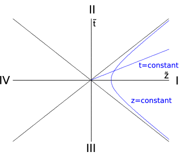
An uniformly accelerated observer viewpoint is described by means of the Rindler coordinates Misner et al. (1973). In order to cover the whole Minkowski space-time, two different sets of coordinates are necessary. These sets of coordinates define two causally disconnected regions in Rindler space-time. If we consider that the uniform acceleration a𝑎a lies on the z𝑧z axis, the new Rindler coordinates (t,x,y,z)𝑡𝑥𝑦𝑧(t,x,y,z) as a function of Minkowski coordinates (t~,x~,y~,z~)~𝑡~𝑥~𝑦~𝑧(\tilde{t},\tilde{x},\tilde{y},\tilde{z}) are

at~=eazsinh(at),az~=eazcosh(at),x~=x,y~=yformulae-sequence𝑎~𝑡superscript𝑒𝑎𝑧𝑎𝑡formulae-sequence𝑎~𝑧superscript𝑒𝑎𝑧𝑎𝑡formulae-sequence~𝑥𝑥~𝑦𝑦a\tilde{t}=e^{az}\sinh(at),\;a\tilde{z}=e^{az}\cosh(at),\;\tilde{x}=x,\;\tilde{y}=y (1)

for region I, and

at~=eazsinh(at),az~=eazcosh(at),x~=x,y~=yformulae-sequence𝑎~𝑡superscript𝑒𝑎𝑧𝑎𝑡formulae-sequence𝑎~𝑧superscript𝑒𝑎𝑧𝑎𝑡formulae-sequence~𝑥𝑥~𝑦𝑦a\tilde{t}=-e^{az}\sinh(at),\;a\tilde{z}=-e^{az}\cosh(at),\;\tilde{x}=x,\;\tilde{y}=y (2)

for region IV.

Refer to caption
Figure 1: (Colour online) Rindler space-time diagram: lines of constant position z=const.𝑧const.z=\text{const.} are hyperbolae and all the curves of constant proper time t𝑡t for the accelerated observer are straight lines that come from the origin. An uniformly accelerated observer Rob travels along a hyperbola constrained to region I

As we can see from fig. 1, although we have covered the whole Minkowski space-time with these sets of coordinates, there are two more regions labeled II and III. To map them we would need to trade cosh\cosh by sinh\sinh in equations (1),(2). In these regions, t𝑡t is a spacelike coordinate and z𝑧z is a timelike coordinate. However, considering such regions is not required to describe fields from an accelerated observer perspective Birrell and Davies (1984); Misner et al. (1973); Fuentes-Schuller and Mann (2005); Alsing et al. (2006); León and Martín-Martínez (2009).

The Rindler coordinates z,t𝑧𝑡z,t go from -\infty to \infty independently in regions I and IV. It means that each region admits a separate quantization procedure with their corresponding positive and negative energy solutions of Klein-Gordon or Dirac equations111Throughout this work we will consider that the spin of each mode lies on the acceleration direction and, hence, spin will not undergo Thomas precession due to instant Wigner rotations Alsing et al. (2006); Jáuregui et al. (1991). {ψk,sI+,ψk,sI}subscriptsuperscript𝜓limit-from𝐼𝑘𝑠subscriptsuperscript𝜓limit-from𝐼𝑘𝑠\{\psi^{I+}_{k,s},\psi^{I-}_{k,s}\} and {ψk,sIV+,ψk,sIV}subscriptsuperscript𝜓limit-from𝐼𝑉𝑘𝑠subscriptsuperscript𝜓limit-from𝐼𝑉𝑘𝑠\{\psi^{IV+}_{k,s},\psi^{IV-}_{k,s}\}.

Particles and antiparticles will be classified with respect to the future-directed timelike Killing vector in each region. In region I the future-directed Killing vector is

tI=t~tt~+z~tz~=a(z~t~+t~z~),superscriptsubscript𝑡𝐼~𝑡𝑡subscript~𝑡~𝑧𝑡subscript~𝑧𝑎~𝑧subscript~𝑡~𝑡subscript~𝑧\partial_{t}^{I}=\frac{\partial\tilde{t}}{\partial t}\partial_{\tilde{t}}+\frac{\partial\tilde{z}}{\partial t}\partial_{\tilde{z}}=a(\tilde{z}\partial_{\tilde{t}}+\tilde{t}\partial_{\tilde{z}}), (3)

whereas in region IV the future-directed Killing vector is tIV=tIsuperscriptsubscript𝑡𝐼𝑉superscriptsubscript𝑡𝐼\partial_{t}^{IV}=-\partial_{t}^{I}.

This means that solutions in region I, having time dependence ψkI+eik0tsimilar-tosuperscriptsubscript𝜓𝑘limit-from𝐼superscript𝑒𝑖subscript𝑘0𝑡\psi_{k}^{I+}\sim e^{-ik_{0}t} with k0>0subscript𝑘00k_{0}>0, represent positive energy solutions, whereas solutions in region IV, having time dependence ψkI+eik0tsimilar-tosuperscriptsubscript𝜓𝑘limit-from𝐼superscript𝑒𝑖subscript𝑘0𝑡\psi_{k}^{I+}\sim e^{-ik_{0}t} with k0>0subscript𝑘00k_{0}>0, are actually negative energy solutions since tIVsubscriptsuperscript𝐼𝑉𝑡\partial^{IV}_{t} points to the opposite direction of t~subscript~𝑡\partial_{\tilde{t}}. As I and IV are causally disconnected ψk,sIV±subscriptsuperscript𝜓limit-from𝐼𝑉plus-or-minus𝑘𝑠\psi^{IV\pm}_{k,s} and ψk,sI±subscriptsuperscript𝜓limit-from𝐼plus-or-minus𝑘𝑠\psi^{I\pm}_{k,s} only have support in their own regions, vanishing outside them.

Let us denote (aI,k,aI,k)superscriptsubscript𝑎𝐼𝑘absentsubscriptsuperscript𝑎𝐼𝑘(a_{I,k}^{\phantom{\dagger}},a^{\dagger}_{I,k}) for the scalar field and (bI,k,s,bI,k,s)subscriptsuperscript𝑏absent𝐼𝑘𝑠subscriptsuperscript𝑏𝐼𝑘𝑠(b^{\phantom{\dagger}}_{I,k,s},b^{\dagger}_{I,k,s}) for the Dirac field as the particle annihilation and creation operators in region I, and (cI,k,s,cI,k,s)subscriptsuperscript𝑐absent𝐼𝑘𝑠subscriptsuperscript𝑐𝐼𝑘𝑠(c^{\phantom{\dagger}}_{I,k,s},c^{\dagger}_{I,k,s}) the corresponding antiparticle Dirac field operators. Analogously we define (aIV,k,aIV,k,bIV,k,s,bIV,k,s,cIV,k,s,cIV,k,s)subscriptsuperscript𝑎absent𝐼𝑉𝑘subscriptsuperscript𝑎𝐼𝑉𝑘subscriptsuperscript𝑏absent𝐼𝑉𝑘𝑠subscriptsuperscript𝑏𝐼𝑉𝑘𝑠subscriptsuperscript𝑐absent𝐼𝑉𝑘𝑠superscriptsubscript𝑐𝐼𝑉𝑘𝑠(a^{\phantom{\dagger}}_{IV,k},a^{\dagger}_{IV,k},b^{\phantom{\dagger}}_{IV,k,s},b^{\dagger}_{IV,k,s},c^{\phantom{\dagger}}_{IV,k,s},c_{IV,k,s}^{\dagger}) as the particle/antiparticle operators in region IV.

The bosonic operators satisfy the commutation relations [aR,k,aR,k]=δRRδkksubscriptsuperscript𝑎absentR𝑘subscriptsuperscript𝑎superscriptRsuperscript𝑘subscript𝛿superscriptRRsubscript𝛿𝑘superscript𝑘[a^{\phantom{\dagger}}_{\text{R},k},a^{\dagger}_{\text{R}^{\prime},k^{\prime}}]=\delta_{\text{R}\text{R}^{\prime}}\delta_{kk^{\prime}} and the fermionic operators satisfy the anticommutation relations {cR,k,s,cR,k,s}=δRRδkkδsssubscriptsuperscript𝑐absentR𝑘𝑠subscriptsuperscript𝑐superscriptRsuperscript𝑘superscript𝑠subscript𝛿superscriptRRsubscript𝛿𝑘superscript𝑘subscript𝛿𝑠superscript𝑠\{c^{\phantom{\dagger}}_{\text{R},k,s},c^{\dagger}_{\text{R}^{\prime},k^{\prime},s^{\prime}}\}=\delta_{\text{R}\text{R}^{\prime}}\delta_{kk^{\prime}}\delta_{ss^{\prime}}. The subscript R notates the Rindler region of the operator R={I,IV}R𝐼𝐼𝑉\text{R}=\{I,IV\}. All other commutators and anticommutators are zero. This includes the anticommutators between operators in different regions of the Rindler space-time.

We can relate Minkowski and Rindler creation and annihilation operators by taking appropriate inner products and computing the so-called Bogoliubov coefficients Takagi (1986); Jáuregui et al. (1991); Birrell and Davies (1984); Alsing et al. (2006).

For a scalar field, the Bogoliubov relationships for the annihilation operator of modes with positive frequency are

aM,ksubscript𝑎𝑀𝑘\displaystyle a_{M,k} =\displaystyle= coshrsaI,ksinhrsaIV,ksubscript𝑟𝑠subscript𝑎𝐼𝑘subscript𝑟𝑠subscriptsuperscript𝑎𝐼𝑉𝑘\displaystyle\cosh r_{s}\,a_{I,k}-\sinh r_{s}\,a^{\dagger}_{IV,-k} (4)

where

tanhrs=eπk0casubscript𝑟𝑠superscript𝑒𝜋subscript𝑘0𝑐𝑎\tanh r_{s}=e^{-\pi\frac{k_{0}c}{a}} (5)

For a Dirac field, the Bogoliubov relationships take the form

bM,k,ssubscript𝑏𝑀𝑘𝑠\displaystyle b_{M,k,s} =\displaystyle= cosrdbI,k,ssinrdcIV,k,ssubscript𝑟𝑑subscript𝑏𝐼𝑘𝑠subscript𝑟𝑑subscriptsuperscript𝑐𝐼𝑉𝑘𝑠\displaystyle\cos{r_{d}}\,b_{I,k,s}-\sin r_{d}\,c^{\dagger}_{IV,-k,-s}
cM,k,ssubscriptsuperscript𝑐𝑀𝑘𝑠\displaystyle c^{\dagger}_{M,k,s} =\displaystyle= cosrdcIV,k,s+sinrdbI,k,ssubscript𝑟𝑑subscriptsuperscript𝑐𝐼𝑉𝑘𝑠subscript𝑟𝑑subscript𝑏𝐼𝑘𝑠\displaystyle\cos{r_{d}}\,c^{\dagger}_{IV,k,s}+\sin r_{d}\,b_{I,-k,-s} (6)

where

tanrs=eπk0casubscript𝑟𝑠superscript𝑒𝜋subscript𝑘0𝑐𝑎\tan r_{s}=e^{-\pi\frac{k_{0}c}{a}} (7)

III Vacuum and one particle states

The Minkowski vacuum state for the scalar field is defined by the tensor product of each frequency mode vacuum

|0=k|0kket0subscripttensor-product𝑘ketsubscript0𝑘\left|{0}\right\rangle=\bigotimes_{k}\left|{0_{k}}\right\rangle (8)

such that it is annihilated by aksubscript𝑎𝑘a_{k} for all values of k𝑘k.

The Minkowski vacuum state for the Dirac field is defined by the tensor product of each frequency mode vacuum

|0=k,ks,s|0k,s+|0k,sket0subscripttensor-product𝑘superscript𝑘𝑠superscript𝑠superscriptketsubscript0𝑘𝑠superscriptketsubscript0superscript𝑘superscript𝑠\left|{0}\right\rangle=\bigotimes_{\begin{subarray}{c}k,k^{\prime}\\ s,s^{\prime}\end{subarray}}\left|{0_{k,s}}\right\rangle^{+}\left|{0_{k^{\prime},s^{\prime}}}\right\rangle^{-} (9)

such that it is annihilated by bk,ssubscript𝑏𝑘𝑠b_{k,s} and ck,ssubscript𝑐𝑘𝑠c_{k,s} for all values of k,s𝑘𝑠k,s. The ±plus-or-minus\pm label indicates particle/antiparticle mode.

For the sake of this work we are going to constrain ourselves to the single mode approximation (SMA) Alsing and Milburn (2003); Alsing et al. (2004). In any case in Martín-Martínez and León (2009) we showed, as an universality principle, that going beyond this approximation does not modify the way in which Unruh decoherence affects entanglement of spinless fermionic and Dirac fields. Specifically, it was shown that Unruh decoherence is independent of the number of modes of the field considered in the analysis, being statistics the ruler of this process. Hence, for our purposes, carrying out this approximation or not will not be relevant.

As it is shown in Fuentes-Schuller and Mann (2005), the vacuum state for a k𝑘k-momentum mode of a scalar field seen from the perspective of an accelerated observer is

|0kM=1coshrsn=0tanhnrs|nkI|nkIVsubscriptketsubscript0𝑘𝑀1subscript𝑟𝑠superscriptsubscript𝑛0superscript𝑛subscript𝑟𝑠subscriptketsubscript𝑛𝑘𝐼subscriptketsubscript𝑛𝑘𝐼𝑉\left|{0_{k}}\right\rangle_{M}=\frac{1}{\cosh r_{s}}\sum_{n=0}^{\infty}\tanh^{n}r_{s}\left|{n_{k}}\right\rangle_{I}\left|{n_{-k}}\right\rangle_{IV} (10)

and as it is shown in León and Martín-Martínez (2009), the vacuum state for a Dirac field seen from the accelerated frame is

|0Msubscriptket0𝑀\displaystyle\left|{0}\right\rangle_{M} =\displaystyle= cos2rd|0kI+|0kIV+sinrdcosrd(|kI+|kIV\displaystyle\cos^{2}r_{d}\,\left|{0}_{k}\right\rangle_{I}^{+}\left|{0}_{k}\right\rangle_{IV}^{-}+\sin r_{d}\,\cos r_{d}\left(\left|{\uparrow}_{k}\right\rangle_{I}^{+}\left|{\downarrow}_{k}\right\rangle_{IV}^{-}\right. (11)
+|kI+|kIV)+sin2rd|pkI+|pkIV\displaystyle\left.+\left|{\downarrow}_{k}\right\rangle_{I}^{+}\left|{\uparrow}_{k}\right\rangle_{IV}^{-}\right)+\sin^{2}r_{d}\,\left|{p}_{k}\right\rangle_{I}^{+}\left|{p}_{k}\right\rangle_{IV}^{-}

where |pk±superscriptketsubscript𝑝𝑘plus-or-minus\left|{p_{k}}\right\rangle^{\pm} represents the pair of particles/antiparticles for frequency k𝑘k as defined below. In these expressions we use the same notation as in references Fuentes-Schuller and Mann (2005); León and Martín-Martínez (2009).

Notice that for fermions there is a constraint due to Pauli exclusion principle

bk,sbk,s|0=|sskδs,ssubscriptsuperscript𝑏𝑘𝑠subscriptsuperscript𝑏𝑘superscript𝑠ket0ket𝑠subscriptsuperscript𝑠𝑘subscript𝛿𝑠superscript𝑠b^{\dagger}_{k,s}b^{\dagger}_{k,s^{\prime}}\left|{0}\right\rangle=\left|{ss^{\prime}_{k}}\right\rangle\delta_{s,{-s^{\prime}}} (12)

If s=s𝑠superscript𝑠s=s^{\prime} the two particle state is not allowed. Therefore the allowed Minkowski states for each mode of particle/antiparticle are

{|0k±,|k±,|k±,|pk±}.superscriptketsubscript0𝑘plus-or-minussuperscriptketsubscript𝑘plus-or-minussuperscriptketsubscript𝑘plus-or-minussuperscriptketsubscript𝑝𝑘plus-or-minus\{\left|{0_{k}}\right\rangle^{\pm},\left|{\uparrow_{k}}\right\rangle^{\pm},\left|{\downarrow_{k}}\right\rangle^{\pm},\left|{p_{k}}\right\rangle^{\pm}\}. (13)

From now on we will drop the sign ±plus-or-minus\pm as, in this work, a mode in region I𝐼I will always be a particle mode and a mode in region IV𝐼𝑉IV will always represent an antiparticle mode. To simplify notation we will also drop the k𝑘k label as we are working under SMA.

We will use the following definitions for a pair of fermions

|pIsubscriptket𝑝𝐼\displaystyle\left|{p}\right\rangle_{I} =\displaystyle= bIbI|0I=bIbI|0Isubscriptsuperscript𝑏𝐼absentsubscriptsuperscript𝑏𝐼absentsubscriptket0𝐼subscriptsuperscript𝑏𝐼absentsubscriptsuperscript𝑏𝐼absentsubscriptket0𝐼\displaystyle b^{\dagger}_{I\uparrow}b^{\dagger}_{I\downarrow}\left|{0}\right\rangle_{I}=-b^{\dagger}_{I\downarrow}b^{\dagger}_{I\uparrow}\left|{0}\right\rangle_{I}
|pIVsubscriptket𝑝𝐼𝑉\displaystyle\left|{p}\right\rangle_{IV} =\displaystyle= cIVcIV|0IV=cIVcIV|0IVsubscriptsuperscript𝑐𝐼𝑉absentsubscriptsuperscript𝑐𝐼𝑉absentsubscriptket0𝐼𝑉subscriptsuperscript𝑐𝐼𝑉absentsubscriptsuperscript𝑐𝐼𝑉absentsubscriptket0𝐼𝑉\displaystyle c^{\dagger}_{IV\uparrow}c^{\dagger}_{IV\downarrow}\left|{0}\right\rangle_{IV}=-c^{\dagger}_{IV\downarrow}c^{\dagger}_{IV\uparrow}\left|{0}\right\rangle_{IV} (14)

and, being consistent with the different Rindler regions operators anticommutation relations,

|sI|sIV=bIscIVs|0I|0IV=cIVsbIs|0I|0IVsubscriptket𝑠𝐼subscriptketsuperscript𝑠𝐼𝑉subscriptsuperscript𝑏𝐼𝑠subscriptsuperscript𝑐𝐼𝑉superscript𝑠subscriptket0𝐼subscriptket0𝐼𝑉subscriptsuperscript𝑐𝐼𝑉superscript𝑠subscriptsuperscript𝑏𝐼𝑠subscriptket0𝐼subscriptket0𝐼𝑉\left|{s}\right\rangle_{I}\left|{s^{\prime}}\right\rangle_{IV}=b^{\dagger}_{Is}c^{\dagger}_{IVs^{\prime}}\left|{0}\right\rangle_{I}\left|{0}\right\rangle_{IV}=-c^{\dagger}_{IVs^{\prime}}b^{\dagger}_{Is}\left|{0}\right\rangle_{I}\left|{0}\right\rangle_{IV}
cIVs|sI|0IV=|sI|sIV.subscriptsuperscript𝑐𝐼𝑉superscript𝑠subscriptket𝑠𝐼subscriptket0𝐼𝑉subscriptket𝑠𝐼subscriptketsuperscript𝑠𝐼𝑉c^{\dagger}_{IVs^{\prime}}\left|{s}\right\rangle_{I}\left|{0}\right\rangle_{IV}=-\left|{s}\right\rangle_{I}\left|{s^{\prime}}\right\rangle_{IV}. (15)

For this work we will also need the Minkowskian one particle state in Rindler coordinates. This state would be

|1M=1cosh2rsn=0tanhnrsn+1|n+1I|nIVsubscriptket1𝑀1superscript2subscript𝑟𝑠superscriptsubscript𝑛0superscript𝑛subscript𝑟𝑠𝑛1subscriptket𝑛1𝐼subscriptket𝑛𝐼𝑉\left|{1}\right\rangle_{M}=\frac{1}{\cosh^{2}r_{s}}\sum_{n=0}^{\infty}\tanh^{n}r_{s}\,\sqrt{n+1}\left|{n+1}\right\rangle_{I}\left|{n}\right\rangle_{IV} (16)

for the scalar field Fuentes-Schuller and Mann (2005) and

|Msubscriptket𝑀\displaystyle\left|{\uparrow}\right\rangle_{M} =\displaystyle= cosrd|I|0IV+sinrd|pI|IVsubscript𝑟𝑑subscriptket𝐼subscriptket0𝐼𝑉subscript𝑟𝑑subscriptket𝑝𝐼subscriptket𝐼𝑉\displaystyle\cos r_{d}\left|{\uparrow}\right\rangle_{I}\left|{0}\right\rangle_{IV}+\sin r_{d}\left|{p}\right\rangle_{I}\left|{\uparrow}\right\rangle_{IV}
|Msubscriptket𝑀\displaystyle\left|{\downarrow}\right\rangle_{M} =\displaystyle= cosrd|I|0IVsinrd|pI|IVsubscript𝑟𝑑subscriptket𝐼subscriptket0𝐼𝑉subscript𝑟𝑑subscriptket𝑝𝐼subscriptket𝐼𝑉\displaystyle\cos r_{d}\left|{\downarrow}\right\rangle_{I}\left|{0}\right\rangle_{IV}-\sin r_{d}\left|{p}\right\rangle_{I}\left|{\downarrow}\right\rangle_{IV} (17)

for the Dirac field León and Martín-Martínez (2009).

Now we need to consider the following maximally entangled states in Minkowsky coordinates

|ΨsketsubscriptΨ𝑠\displaystyle\left|{\Psi_{s}}\right\rangle =\displaystyle= 12(|0M|0M+|1M|1M)12subscriptket0𝑀subscriptket0𝑀subscriptket1𝑀subscriptket1𝑀\displaystyle\frac{1}{\sqrt{2}}\left(\left|{0}\right\rangle_{M}\left|{0}\right\rangle_{M}+\left|{1}\right\rangle_{M}\left|{1}\right\rangle_{M}\right) (18)
|ΨdketsubscriptΨ𝑑\displaystyle\left|{\Psi_{d}}\right\rangle =\displaystyle= 12(|0M|0M+|M|M)12subscriptket0𝑀subscriptket0𝑀subscriptket𝑀subscriptket𝑀\displaystyle\frac{1}{\sqrt{2}}\left(\left|{0}\right\rangle_{M}\left|{0}\right\rangle_{M}+\left|{\uparrow}\right\rangle_{M}\left|{\downarrow}\right\rangle_{M}\right) (19)

These two maximally entangled states are analogous, both are qubit states and superpositions of the bipartitie vacuum and the bipartite one particle state. The difference is that in (19) we have a Dirac field state and hence, the one particle states have spin.

For |ΨdketsubscriptΨ𝑑\left|{\Psi_{d}}\right\rangle we have selected one amongst the possible values for the spin of the terms with one particle for Alice and Rob, but it can be shown that the election of a specific value for these spins is not relevant when considering the behaviour of corrleations. Then, the results presented here are independent of the particular choice of a spin state for the superposition (19).

IV Correlations for the Dirac field

The density matrix for whole tripartite state, which includes modes on both sides of the Rindler horizon along with Minkowskian modes, is built from (19)

ρdARR¯=|ΨdΨd|subscriptsuperscript𝜌𝐴𝑅¯𝑅𝑑ketsubscriptΨ𝑑brasubscriptΨ𝑑\rho^{AR\bar{R}}_{d}=\left|{\Psi_{d}}\right\rangle\!\left\langle{\Psi_{d}}\right| (20)

The three different bipartitions for the Dirac field case are obtained by partial tracing over the part which we want to eliminate, which is to say.

ρdARsubscriptsuperscript𝜌𝐴𝑅𝑑\displaystyle\rho^{AR}_{d} =\displaystyle\!\!=\! TrIVρdARR¯=s{0,,,p}s|IVρdARR¯|sIVsubscriptTr𝐼𝑉subscriptsuperscript𝜌𝐴𝑅¯𝑅𝑑subscript𝑠0𝑝subscriptbra𝑠𝐼𝑉superscriptsubscript𝜌𝑑𝐴𝑅¯𝑅subscriptket𝑠𝐼𝑉\displaystyle\operatorname{Tr}_{IV}\rho^{AR\bar{R}}_{d}=\!\!\!\!\sum_{s\in\{0,\uparrow,\downarrow,p\}}\left\langle{s}\right|_{IV}\rho_{d}^{AR\bar{R}}\left|{s}\right\rangle_{IV} (21)
ρdAR¯subscriptsuperscript𝜌𝐴¯𝑅𝑑\displaystyle\rho^{A\bar{R}}_{d} =\displaystyle\!\!=\! TrIρdARR¯=s{0,,,p}s|IρdARR¯|sIsubscriptTr𝐼subscriptsuperscript𝜌𝐴𝑅¯𝑅𝑑subscript𝑠0𝑝subscriptbra𝑠𝐼superscriptsubscript𝜌𝑑𝐴𝑅¯𝑅subscriptket𝑠𝐼\displaystyle\operatorname{Tr}_{I}\rho^{AR\bar{R}}_{d}=\!\!\!\!\sum_{s\in\{0,\uparrow,\downarrow,p\}}\left\langle{s}\right|_{I}\rho_{d}^{AR\bar{R}}\left|{s}\right\rangle_{I} (22)
ρdRR¯subscriptsuperscript𝜌𝑅¯𝑅𝑑\displaystyle\rho^{R\bar{R}}_{d} =\displaystyle\!\!=\! TrMρdARR¯=s{0,,,p}s|MρdARR¯|sMsubscriptTr𝑀subscriptsuperscript𝜌𝐴𝑅¯𝑅𝑑subscript𝑠0𝑝subscriptbra𝑠𝑀superscriptsubscript𝜌𝑑𝐴𝑅¯𝑅subscriptket𝑠𝑀\displaystyle\operatorname{Tr}_{M}\rho^{AR\bar{R}}_{d}=\!\!\!\!\sum_{s\in\{0,\uparrow,\downarrow,p\}}\left\langle{s}\right|_{M}\rho_{d}^{AR\bar{R}}\left|{s}\right\rangle_{M} (23)

and the density matrix for each individual subsystem is obtained by tracing over the other subsystems,

ρdAsubscriptsuperscript𝜌𝐴𝑑\displaystyle\rho^{A}_{d} =\displaystyle= TrIρdAR=TrIVρdAR¯subscriptTr𝐼subscriptsuperscript𝜌𝐴𝑅𝑑subscriptTr𝐼𝑉subscriptsuperscript𝜌𝐴¯𝑅𝑑\displaystyle\operatorname{Tr}_{I}\rho^{AR}_{d}=\operatorname{Tr}_{IV}\rho^{A\bar{R}}_{d} (24)
ρdRsubscriptsuperscript𝜌𝑅𝑑\displaystyle\rho^{R}_{d} =\displaystyle= TrIVρdRR¯=TrMρdARsubscriptTr𝐼𝑉subscriptsuperscript𝜌𝑅¯𝑅𝑑subscriptTr𝑀subscriptsuperscript𝜌𝐴𝑅𝑑\displaystyle\operatorname{Tr}_{IV}\rho^{R\bar{R}}_{d}=\operatorname{Tr}_{M}\rho^{AR}_{d} (25)
ρdR¯subscriptsuperscript𝜌¯𝑅𝑑\displaystyle\rho^{\bar{R}}_{d} =\displaystyle= TrIρdRR¯=TrMρdAR¯subscriptTr𝐼subscriptsuperscript𝜌𝑅¯𝑅𝑑subscriptTr𝑀subscriptsuperscript𝜌𝐴¯𝑅𝑑\displaystyle\operatorname{Tr}_{I}\rho^{R\bar{R}}_{d}=\operatorname{Tr}_{M}\rho^{A\bar{R}}_{d} (26)

The different bipartitions are characterized by the following density matrices

ρdARsubscriptsuperscript𝜌𝐴𝑅𝑑\displaystyle\rho^{AR}_{d} =\displaystyle= 12[cos4rd|0000|+sin2rdcos2rd(|00|\displaystyle\frac{1}{2}\Big{[}\cos^{4}r_{d}\left|{00}\right\rangle\!\left\langle{00}\right|+\sin^{2}r_{d}\,\cos^{2}r_{d}\Big{(}\left|{0\uparrow}\right\rangle\!\left\langle{0\uparrow}\right| (27)
+|00|)+sin4rd|0p0p|+cos3rd(|00\displaystyle\!\!\!+\left|{0\downarrow}\right\rangle\!\left\langle{0\downarrow}\right|\Big{)}+\sin^{4}r_{d}\left|{0p}\right\rangle\!\left\langle{0p}\right|+\cos^{3}r_{d}\Big{(}\left|{00}\right\rangle
×|+|00|)sin2rdcosrd(|0p|\displaystyle\!\!\!\times\left\langle{\uparrow\downarrow}\right|+\left|{\uparrow\downarrow}\right\rangle\!\left\langle{00}\right|\Big{)}-\sin^{2}r_{d}\cos r_{d}\Big{(}\left|{0\uparrow}\right\rangle\!\left\langle{\uparrow p}\right|
+|p0|)+cos2rd||+sin2rd\displaystyle+\left|{\uparrow p}\right\rangle\!\left\langle{0\uparrow}\right|\Big{)}+\cos^{2}r_{d}\left|{\uparrow\downarrow}\right\rangle\!\left\langle{\uparrow\downarrow}\right|+\sin^{2}r_{d}
×|pp|]\displaystyle\times\left|{\uparrow p}\right\rangle\!\left\langle{\uparrow p}\right|\Big{]}
ρdAR¯subscriptsuperscript𝜌𝐴¯𝑅𝑑\displaystyle\rho^{A\bar{R}}_{d} =\displaystyle= 12[cos4rd|0000|+sin2rdcos2rd(|00|\displaystyle\frac{1}{2}\Big{[}\cos^{4}r_{d}\left|{00}\right\rangle\!\left\langle{00}\right|+\sin^{2}r_{d}\,\cos^{2}r_{d}\Big{(}\left|{0\downarrow}\right\rangle\!\left\langle{0\downarrow}\right| (28)
+|00|)+sin4rd|0p0p|sin3rd\displaystyle\!\!\!+\left|{0\uparrow}\right\rangle\!\left\langle{0\uparrow}\right|\Big{)}+\sin^{4}r_{d}\left|{0p}\right\rangle\!\left\langle{0p}\right|-\sin^{3}r_{d}
×(|0p|+|0p|)+sinrdcos2rd(|0\displaystyle\!\!\!\times\Big{(}\left|{0p}\right\rangle\!\left\langle{\uparrow\downarrow}\right|+\left|{\uparrow\downarrow}\right\rangle\!\left\langle{0p}\right|\Big{)}+\sin r_{d}\cos^{2}r_{d}\Big{(}\left|{0\uparrow}\right\rangle
×0|+|00|)+cos2rd|00|\displaystyle\times\left\langle{\uparrow 0}\right|+\left|{\uparrow 0}\right\rangle\!\left\langle{0\uparrow}\right|\Big{)}+\cos^{2}r_{d}\left|{\uparrow 0}\right\rangle\!\left\langle{\uparrow 0}\right|
+sin2rd||]\displaystyle+\sin^{2}r_{d}\left|{\uparrow\downarrow}\right\rangle\!\left\langle{\uparrow\downarrow}\right|\Big{]}
ρdRR¯subscriptsuperscript𝜌𝑅¯𝑅𝑑\displaystyle\rho^{R\bar{R}}_{d}\!\!\! =\displaystyle= 12[cos4rd|0000|+sinrdcos3rd(|00|+|00\displaystyle\!\!\!\frac{1}{2}\Big{[}\cos^{4}r_{d}\left|{00}\right\rangle\!\left\langle{00}\right|+\sin r_{d}\,\cos^{3}r_{d}\Big{(}\left|{00}\right\rangle\!\left\langle{\uparrow\downarrow}\right|+\left|{00}\right\rangle (29)
×|+|00|+|00|)+sin2rdcos2rd(|00\displaystyle\!\!\!\!\!\times\left\langle{\downarrow\uparrow}\right|+\left|{\uparrow\downarrow}\right\rangle\!\left\langle{00}\right|+\left|{\downarrow\uparrow}\right\rangle\!\left\langle{00}\right|\Big{)}+\sin^{2}r_{d}\cos^{2}r_{d}\Big{(}\left|{00}\right\rangle
×pp|+||+||+||+||\displaystyle\!\!\!\!\!\times\left\langle{pp}\right|\!+\!\left|{\uparrow\downarrow}\right\rangle\!\left\langle{\uparrow\downarrow}\right|\!+\!\left|{\uparrow\downarrow}\right\rangle\!\left\langle{\downarrow\uparrow}\right|\!+\!\left|{\downarrow\uparrow}\right\rangle\!\left\langle{\uparrow\downarrow}\right|\!+\!\left|{\downarrow\uparrow}\right\rangle\!\left\langle{\downarrow\uparrow}\right|
+|pp00|)+sin3rdcosrd(|pp|\displaystyle\!\!\!\!\!+\left|{pp}\right\rangle\!\left\langle{00}\right|\Big{)}+\sin^{3}r_{d}\,\cos r_{d}\Big{(}\left|{\uparrow\downarrow}\right\rangle\!\left\langle{pp}\right|
+|pp|+|pp|+|pp|)\displaystyle\!\!\!\!\!+\left|{pp}\right\rangle\!\left\langle{\uparrow\downarrow}\right|+\left|{\downarrow\uparrow}\right\rangle\left\langle{pp}\right|\!+\!\left|{pp}\right\rangle\!\left\langle{\downarrow\uparrow}\right|\Big{)}
+cos2rd|00|+sin2rd|pp|\displaystyle\!\!\!\!\!+\cos^{2}r_{d}\left|{\downarrow 0}\right\rangle\!\left\langle{\downarrow 0}\right|+\sin^{2}r_{d}\left|{p\downarrow}\right\rangle\!\left\langle{p\downarrow}\right|
cosrdsinrd(|0p|+|p0|)\displaystyle\!\!\!\!\!-\cos r_{d}\,\sin r_{d}\Big{(}\left|{\downarrow 0}\right\rangle\!\left\langle{p\downarrow}\right|+\left|{p\downarrow}\right\rangle\left\langle{\downarrow 0}\right|\Big{)}
+sin4rd|pppp|]\displaystyle\!\!\!\!\!+\sin^{4}r_{d}\left|{pp}\right\rangle\!\left\langle{pp}\right|\Big{]}

where the bases are

|nmket𝑛𝑚\displaystyle\left|{nm}\right\rangle =\displaystyle= |nAM|mRIsubscriptketsuperscript𝑛𝐴𝑀subscriptketsuperscript𝑚𝑅𝐼\displaystyle\left|{n^{A}}\right\rangle_{M}\left|{m^{R}}\right\rangle_{I} (30)
|nmket𝑛𝑚\displaystyle\left|{nm}\right\rangle =\displaystyle= |nAM|mR¯IVsubscriptketsuperscript𝑛𝐴𝑀subscriptketsuperscript𝑚¯𝑅𝐼𝑉\displaystyle\left|{n^{A}}\right\rangle_{M}|m^{\bar{R}}\rangle_{IV} (31)
|nmket𝑛𝑚\displaystyle\left|{nm}\right\rangle =\displaystyle= |nRI|mR¯IVsubscriptketsuperscript𝑛𝑅𝐼subscriptketsuperscript𝑚¯𝑅𝐼𝑉\displaystyle\left|{n^{R}}\right\rangle_{I}|m^{\bar{R}}\rangle_{IV} (32)

respectively for (27), (28) and (29).

On the other hand, the density matrices for the individual subsystems (24), (25),(26) are

ρdRsubscriptsuperscript𝜌𝑅𝑑\displaystyle\rho^{R}_{d} =\displaystyle= 12[sin2rd(1+sin2rd)|pp|+sin2rdcos2rd||\displaystyle\frac{1}{2}\Big{[}\sin^{2}r_{d}(1+\sin^{2}r_{d})\left|{p}\right\rangle\!\left\langle{p}\right|+\sin^{2}r_{d}\cos^{2}r_{d}\left|{\uparrow}\right\rangle\!\left\langle{\uparrow}\right| (33)
+cos2rd(1+sin2rd)||+cos4rd|00|]\displaystyle+\cos^{2}r_{d}(1+\sin^{2}r_{d})\left|{\downarrow}\right\rangle\!\left\langle{\downarrow}\right|+\cos^{4}r_{d}\left|{0}\right\rangle\!\left\langle{0}\right|\Big{]}
ρdR¯subscriptsuperscript𝜌¯𝑅𝑑\displaystyle\rho^{\bar{R}}_{d} =\displaystyle= 12[cos2rd(1+cos2rd)|00|+sin2rdcos2rd||\displaystyle\frac{1}{2}\Big{[}\cos^{2}r_{d}(1+\cos^{2}r_{d})\left|{0}\right\rangle\!\left\langle{0}\right|+\sin^{2}r_{d}\cos^{2}r_{d}\left|{\uparrow}\right\rangle\!\left\langle{\uparrow}\right| (34)
+sin2rd(1+cos2rd)||+sin4rd|pp|]\displaystyle+\sin^{2}r_{d}(1+\cos^{2}r_{d})\left|{\downarrow}\right\rangle\!\left\langle{\downarrow}\right|+\sin^{4}r_{d}\left|{p}\right\rangle\!\left\langle{p}\right|\Big{]}
ρdA=12(|00|+||)\rho^{A}_{d}=\frac{1}{2}\left(\left|{0}\right\rangle\!\left\langle{0}\right|+\left|{\uparrow}\right\rangle\!\left\langle{\uparrow}\right|\right) (35)

IV.1 Mutual Information: creation, exchange and conservation

Mutual information accounts for correlations (both quantum and classical) between two different parts of a system. It is defined as

IAB=SA+SBSABsubscript𝐼𝐴𝐵subscript𝑆𝐴subscript𝑆𝐵subscript𝑆𝐴𝐵I_{AB}=S_{A}+S_{B}-S_{AB} (36)

where SAsubscript𝑆𝐴S_{A}, SBsubscript𝑆𝐵S_{B} and SABsubscript𝑆𝐴𝐵S_{AB} are respectively the Von Neuman entropies for the individual subsystems A𝐴A and B𝐵B and for the joint system AB𝐴𝐵AB.

To compute the mutual information for each bipartition we will need the eigenvalues of the corresponding density matrices. We shall go through all the process step by step in the lines below.

IV.1.1 Bipartition Alice-Rob

The eigenvalues of the matrix for the system Alice-Rob (27) are

λ1subscript𝜆1\displaystyle\lambda_{1} =\displaystyle= λ2=0subscript𝜆20\displaystyle\lambda_{2}=0
λ3subscript𝜆3\displaystyle\lambda_{3} =\displaystyle= 12sin2rdcos2rd12superscript2subscript𝑟𝑑superscript2subscript𝑟𝑑\displaystyle\frac{1}{2}\sin^{2}r_{d}\cos^{2}r_{d}
λ4subscript𝜆4\displaystyle\lambda_{4} =\displaystyle= 12sin4rd12superscript4subscript𝑟𝑑\displaystyle\frac{1}{2}\sin^{4}r_{d}
λ5subscript𝜆5\displaystyle\lambda_{5} =\displaystyle= 12cos2rd(1+cos2rd)12superscript2subscript𝑟𝑑1superscript2subscript𝑟𝑑\displaystyle\frac{1}{2}\cos^{2}r_{d}\left(1+\cos^{2}r_{d}\right)
λ6subscript𝜆6\displaystyle\lambda_{6} =\displaystyle= 12sin2rd(1+cos2rd)12superscript2subscript𝑟𝑑1superscript2subscript𝑟𝑑\displaystyle\frac{1}{2}\sin^{2}r_{d}\left(1+\cos^{2}r_{d}\right) (37)

IV.1.2 Bipartition Alice-AntiRob

The eigenvalues of the matrix for the system Alice-AntiRob (28) are

λ1subscript𝜆1\displaystyle\lambda_{1} =\displaystyle= λ2=0subscript𝜆20\displaystyle\lambda_{2}=0
λ3subscript𝜆3\displaystyle\lambda_{3} =\displaystyle= 12sin2rdcos2rd12superscript2subscript𝑟𝑑superscript2subscript𝑟𝑑\displaystyle\frac{1}{2}\sin^{2}r_{d}\cos^{2}r_{d}
λ4subscript𝜆4\displaystyle\lambda_{4} =\displaystyle= 12cos4rd12superscript4subscript𝑟𝑑\displaystyle\frac{1}{2}\cos^{4}r_{d}
λ5subscript𝜆5\displaystyle\lambda_{5} =\displaystyle= 12sin2rd(1+sin2rd)12superscript2subscript𝑟𝑑1superscript2subscript𝑟𝑑\displaystyle\frac{1}{2}\sin^{2}r_{d}\left(1+\sin^{2}r_{d}\right)
λ6subscript𝜆6\displaystyle\lambda_{6} =\displaystyle= 12cos2rd(1+sin2rd)12superscript2subscript𝑟𝑑1superscript2subscript𝑟𝑑\displaystyle\frac{1}{2}\cos^{2}r_{d}\left(1+\sin^{2}r_{d}\right) (38)

IV.1.3 Bipartition Rob-AntiRob

All the eigenvalues of the matrix for the system Rob-AntiRob (29) are zero excepting two of them

λ1=λ2=12;λi>2=0formulae-sequencesubscript𝜆1subscript𝜆212subscript𝜆𝑖20\lambda_{1}=\lambda_{2}=\frac{1}{2};\qquad\lambda_{i>2}=0 (39)

IV.1.4 Von Neumann entropies for each subsystem and mutual information

To compute the Von Neumann entropies we need the eigenvalues of every bipartition and the individual density matrices. The eigenvalues of ρdARsubscriptsuperscript𝜌𝐴𝑅𝑑\rho^{AR}_{d}, ρdAR¯subscriptsuperscript𝜌𝐴¯𝑅𝑑\rho^{A\bar{R}}_{d}, ρdRR¯subscriptsuperscript𝜌𝑅¯𝑅𝑑\rho^{R\bar{R}}_{d} are respectively (IV.1.1), (IV.1.2) and (39).

The eigevalues of the individual systems density matrices can be directly read from (33), (34) and (35) since ρsRsubscriptsuperscript𝜌𝑅𝑠\rho^{R}_{s}, ρsR¯subscriptsuperscript𝜌¯𝑅𝑠\rho^{\bar{R}}_{s} and ρsAsubscriptsuperscript𝜌𝐴𝑠\rho^{A}_{s} have diagonal forms in the given basis.

The Von Neumann entropy for a partition B𝐵B of the system is

SB=Tr(ρlog2ρ)=λilog2λisubscript𝑆𝐵Tr𝜌subscript2𝜌subscript𝜆𝑖subscript2subscript𝜆𝑖S_{B}=-\operatorname{Tr}(\rho\log_{2}\rho)=-\sum\lambda_{i}\log_{2}\lambda_{i} (40)

At this point, computing the entropies is quite straightforward. The Von Neumann entropies for all the partial systems are

SRsubscript𝑆𝑅\displaystyle S_{R} =\displaystyle= 1sin2rdlog2(sin2rd)32cos2rdlog2(cos2rd)1superscript2subscript𝑟𝑑subscript2superscript2subscript𝑟𝑑32superscript2subscript𝑟𝑑subscript2superscript2subscript𝑟𝑑\displaystyle 1-\sin^{2}r_{d}\log_{2}(\sin^{2}r_{d})-\frac{3}{2}\cos^{2}r_{d}\log_{2}(\cos^{2}r_{d})
1+sin2rd2log2(1+sin2rd)1superscript2subscript𝑟𝑑2subscript21superscript2subscript𝑟𝑑\displaystyle-\frac{1+\sin^{2}r_{d}}{2}\log_{2}(1+\sin^{2}r_{d})
SR¯subscript𝑆¯𝑅\displaystyle S_{\bar{R}} =\displaystyle= 1cos2rdlog2(cos2rd)32sin2rdlog2(sin2rd)1superscript2subscript𝑟𝑑subscript2superscript2subscript𝑟𝑑32superscript2subscript𝑟𝑑subscript2superscript2subscript𝑟𝑑\displaystyle 1-\cos^{2}r_{d}\log_{2}(\cos^{2}r_{d})-\frac{3}{2}\sin^{2}r_{d}\log_{2}(\sin^{2}r_{d})
1+cos2rd2log2(1+cos2rd)1superscript2subscript𝑟𝑑2subscript21superscript2subscript𝑟𝑑\displaystyle-\frac{1+\cos^{2}r_{d}}{2}\log_{2}(1+\cos^{2}r_{d})
SARsubscript𝑆𝐴𝑅\displaystyle S_{AR} =\displaystyle= SR¯;SAR¯=SR;SRR¯=SA=1formulae-sequencesubscript𝑆¯𝑅subscript𝑆𝐴¯𝑅subscript𝑆𝑅subscript𝑆𝑅¯𝑅subscript𝑆𝐴1\displaystyle S_{\bar{R}};\qquad S_{A\bar{R}}=S_{R};\qquad S_{R\bar{R}}=S_{A}=1 (41)

And then, the mutual information for all the possible bipartitions of the system will be

IARsubscript𝐼𝐴𝑅\displaystyle I_{AR} =\displaystyle= SA+SRSAR=1+SRSR¯subscript𝑆𝐴subscript𝑆𝑅subscript𝑆𝐴𝑅1subscript𝑆𝑅subscript𝑆¯𝑅\displaystyle S_{A}+S_{R}-S_{AR}=1+S_{R}-S_{\bar{R}}
IAR¯subscript𝐼𝐴¯𝑅\displaystyle I_{A\bar{R}} =\displaystyle= SA+SR¯SAR¯=1+SR¯SRsubscript𝑆𝐴subscript𝑆¯𝑅subscript𝑆𝐴¯𝑅1subscript𝑆¯𝑅subscript𝑆𝑅\displaystyle S_{A}+S_{\bar{R}}-S_{A\bar{R}}=1+S_{\bar{R}}-S_{R}
IRR¯subscript𝐼𝑅¯𝑅\displaystyle I_{R\bar{R}} =\displaystyle= SR+SR¯SRR¯=SR+SR¯1subscript𝑆𝑅subscript𝑆¯𝑅subscript𝑆𝑅¯𝑅subscript𝑆𝑅subscript𝑆¯𝑅1\displaystyle S_{R}+S_{\bar{R}}-S_{R\bar{R}}=S_{R}+S_{\bar{R}}-1

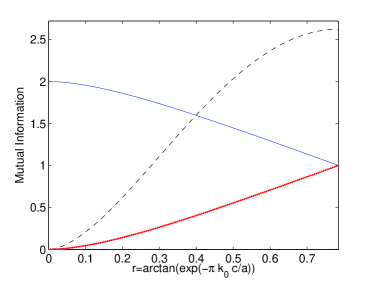
At first glance we can see a conservation law of the mutual information for the system Alice-Rob and Alice-AntiRob

IAR+IAR¯=2subscript𝐼𝐴𝑅subscript𝐼𝐴¯𝑅2I_{AR}+I_{A\bar{R}}=2 (42)

which suggests a correlations transfer from the system Alice-Rob to Alice-AntiRob as the acceleration increases.

Fig. 2 shows the behaviour of the mutual information for the three bipartitions. It also shows how the correlations across the horizon (Rob and AntiRob) increase, up to certain finite limit, as Rob accelerates.

If we recall the results on spinless fermion fields Alsing et al. (2006) we see that the results for Alice-Rob and Alice-AntiRob are exactly the same as those obtained in Alsing et al. (2006), being the conservation law obtained here also valid for that spinless fermion case. This result was expected according to the universality argument adduced in Martín-Martínez and León (2009) as the explanation for the Unruh decoherence for fermion fields of arbitrary spin.

However, something different occurs with the system Rob-AntiRob. The creation of correlations between modes on both sides of the horizon is greater in the Dirac field case. This is related with the dimension of the Hilbert space. As we will see in more detail later, the dimension of the Hilbert space plays a determinant role only in the comportment of the correlations Rob-AntiRob.

IV.2 Entanglement conservation and behaviour across the horizon

We will use the negativity to account for the distillable entanglement of the different bipartitions of the system. Negativity is an entangle monotone which is only sensitive to distillable entanglement.

Negativity is defined as the sum of the negative eigenvalues of the partial transpose density matrix for the system, which is defined as the transpose of only one of the subsystem q-dits in the bipartite density matrix. If σisubscript𝜎𝑖\sigma_{i} are the eigenvalues of ρABpTsubscriptsuperscript𝜌𝑝𝑇𝐴𝐵\rho^{pT}_{AB} then

𝒩AB=12i(|σi|σi)=σi<0σisubscript𝒩𝐴𝐵12subscript𝑖subscript𝜎𝑖subscript𝜎𝑖subscriptsubscript𝜎𝑖0subscript𝜎𝑖\mathcal{N}_{AB}=\frac{1}{2}\sum_{i}(|\sigma_{i}|-\sigma_{i})=-\sum_{\sigma_{i}<0}\sigma_{i} (43)

Therefore, to compute it, we will need the partial transpose of the bipartite density matrices (27), (28) and (29), which we will notate as ηdARsubscriptsuperscript𝜂𝐴𝑅𝑑\eta^{AR}_{d}, ηdAR¯subscriptsuperscript𝜂𝐴¯𝑅𝑑\eta^{A\bar{R}}_{d} and ηdRR¯subscriptsuperscript𝜂𝑅¯𝑅𝑑\eta^{R\bar{R}}_{d} respectively.

ηdARsubscriptsuperscript𝜂𝐴𝑅𝑑\displaystyle\eta^{AR}_{d} =\displaystyle= 12[cos4rd|0000|+sin2rdcos2rd(|00|\displaystyle\frac{1}{2}\Big{[}\cos^{4}r_{d}\left|{00}\right\rangle\!\left\langle{00}\right|+\sin^{2}r_{d}\cos^{2}r_{d}\left(\left|{0\uparrow}\right\rangle\!\left\langle{0\uparrow}\right|\right. (44)
+|00|)+sin4rd|0p0p|+cos3rd\displaystyle\left.+\left|{0\downarrow}\right\rangle\!\left\langle{0\downarrow}\right|\right)+\sin^{4}r_{d}\left|{0p}\right\rangle\!\left\langle{0p}\right|+\cos^{3}r_{d}
×(|00|+|00|)sin2rdcosrd\displaystyle\times\left(\left|{0\downarrow}\right\rangle\!\left\langle{\uparrow 0}\right|+\left|{\uparrow 0}\right\rangle\!\left\langle{0\downarrow}\right|\right)-\sin^{2}r_{d}\,\cos r_{d}
×(|0p|+|0p|)+cos2rd||\displaystyle\times\left(\left|{0p}\right\rangle\!\left\langle{\uparrow\uparrow}\right|+\left|{\uparrow\uparrow}\right\rangle\!\left\langle{0p}\right|\right)+\cos^{2}r_{d}\left|{\uparrow\downarrow}\right\rangle\!\left\langle{\uparrow\downarrow}\right|
+sin2rd|pp|]\displaystyle+\sin^{2}r_{d}\left|{\uparrow p}\right\rangle\!\left\langle{\uparrow p}\right|\Big{]}
ηdAR¯subscriptsuperscript𝜂𝐴¯𝑅𝑑\displaystyle\eta^{A\bar{R}}_{d} =\displaystyle= 12[cos4rd|0000|+sin2rdcos2rd(|00|\displaystyle\frac{1}{2}\Big{[}\cos^{4}r_{d}\left|{00}\right\rangle\!\left\langle{00}\right|+\sin^{2}r_{d}\,\cos^{2}r_{d}\Big{(}\left|{0\downarrow}\right\rangle\!\left\langle{0\downarrow}\right| (45)
+|00|)+sin4rd|0p0p|sin3rd\displaystyle\!\!\!+\left|{0\uparrow}\right\rangle\!\left\langle{0\uparrow}\right|\Big{)}+\sin^{4}r_{d}\left|{0p}\right\rangle\!\left\langle{0p}\right|-\sin^{3}r_{d}
×(|0p|+|p0|)+sinrdcos2rd\displaystyle\!\!\!\times\Big{(}\left|{0\downarrow}\right\rangle\!\left\langle{\uparrow p}\right|+\left|{\uparrow p}\right\rangle\!\left\langle{0\downarrow}\right|\Big{)}+\sin r_{d}\cos^{2}r_{d}
×(|00|+|00|)+cos2rd|00|\displaystyle\times\Big{(}\left|{00}\right\rangle\left\langle{\uparrow\uparrow}\right|+\left|{\uparrow\uparrow}\right\rangle\!\left\langle{00}\right|\Big{)}+\cos^{2}r_{d}\left|{\uparrow 0}\right\rangle\!\left\langle{\uparrow 0}\right|
+sin2rd||]\displaystyle+\sin^{2}r_{d}\left|{\uparrow\downarrow}\right\rangle\!\left\langle{\uparrow\downarrow}\right|\Big{]}
ηdRR¯subscriptsuperscript𝜂𝑅¯𝑅𝑑\displaystyle\eta^{R\bar{R}}_{d}\!\!\! =\displaystyle= 12[cos4rd|0000|+sinrdcos3rd(|00|\displaystyle\!\!\!\frac{1}{2}\Big{[}\cos^{4}r_{d}\left|{00}\right\rangle\!\left\langle{00}\right|+\sin r_{d}\,\cos^{3}r_{d}\Big{(}\left|{0\downarrow}\right\rangle\!\left\langle{\uparrow 0}\right| (46)
+|00|+|00|+|00|)+sin2rd\displaystyle\!\!\!\!\!+\left|{0\uparrow}\right\rangle\left\langle{\downarrow 0}\right|+\left|{\uparrow 0}\right\rangle\!\left\langle{0\downarrow}\right|+\left|{\downarrow 0}\right\rangle\!\left\langle{0\uparrow}\right|\Big{)}+\sin^{2}r_{d}
×cos2rd(|0pp0|+||+||\displaystyle\!\!\!\!\!\times\cos^{2}r_{d}\Big{(}\left|{0p}\right\rangle\left\langle{p0}\right|\!+\!\left|{\uparrow\downarrow}\right\rangle\!\left\langle{\uparrow\downarrow}\right|\!+\!\left|{\uparrow\uparrow}\right\rangle\!\left\langle{\downarrow\downarrow}\right|
+||+||+|p00p|)+sin3rd\displaystyle\!\!\!\!\!+\left|{\downarrow\downarrow}\right\rangle\!\left\langle{\uparrow\uparrow}\right|+\left|{\downarrow\uparrow}\right\rangle\!\left\langle{\downarrow\uparrow}\right|+\left|{p0}\right\rangle\!\left\langle{0p}\right|\Big{)}+\sin^{3}r_{d}
×cosrd(|pp|+|pp|+|pp|\displaystyle\!\!\!\!\!\times\cos r_{d}\Big{(}\left|{\uparrow p}\right\rangle\!\left\langle{p\downarrow}\right|+\left|{p\downarrow}\right\rangle\!\left\langle{\uparrow p}\right|+\left|{\downarrow p}\right\rangle\left\langle{p\uparrow}\right|
+|pp|)+cos2rd|00|+sin2rd|p\displaystyle\!\!\!\!\!+\left|{p\uparrow}\right\rangle\!\left\langle{\downarrow p}\right|\Big{)}+\cos^{2}r_{d}\left|{\downarrow 0}\right\rangle\!\left\langle{\downarrow 0}\right|+\sin^{2}r_{d}\left|{p\downarrow}\right\rangle
×p|cosrdsinrd(|p0|+|p0|)\displaystyle\!\!\!\!\!\times\left\langle{p\downarrow}\right|-\cos r_{d}\,\sin r_{d}\Big{(}\left|{\downarrow\downarrow}\right\rangle\!\left\langle{p0}\right|+\left|{p0}\right\rangle\left\langle{\downarrow\downarrow}\right|\Big{)}
+sin4rd|pppp|]\displaystyle\!\!\!\!\!+\sin^{4}r_{d}\left|{pp}\right\rangle\!\left\langle{pp}\right|\Big{]}

In the following subsections we shall compute the negativity for each bipartition of the system.

IV.2.1 Bipartition Alice-Rob

The eigenvalues of the partial transpose density matrix for the bipartition Alice-Rob (44) turn out to be

λ1subscript𝜆1\displaystyle\lambda_{1} =\displaystyle= 12cos4rd;λ2=12cos2rsin2rd12superscript4subscript𝑟𝑑subscript𝜆212superscript2𝑟superscript2subscript𝑟𝑑\displaystyle\frac{1}{2}\cos^{4}r_{d};\qquad\lambda_{2}=\frac{1}{2}\cos^{2}r\sin^{2}r_{d}
λ3subscript𝜆3\displaystyle\lambda_{3} =\displaystyle= 12sin2rd;λ4=12cos2rd12superscript2subscript𝑟𝑑subscript𝜆412superscript2subscript𝑟𝑑\displaystyle\frac{1}{2}\sin^{2}r_{d};\qquad\lambda_{4}=\frac{1}{2}\cos^{2}r_{d}
λ5,6subscript𝜆56\displaystyle\lambda_{5,6} =\displaystyle= 14sin2rdcos2rd(1±1+4cos2rdsin4r)14superscript2subscript𝑟𝑑superscript2subscript𝑟𝑑plus-or-minus114superscript2subscript𝑟𝑑superscript4𝑟\displaystyle\frac{1}{4}\sin^{2}r_{d}\cos^{2}r_{d}\left(1\pm\sqrt{1+\frac{4\cos^{2}r_{d}}{\sin^{4}r}}\right)
λ7,8subscript𝜆78\displaystyle\lambda_{7,8} =\displaystyle= 14sin4rd(1±1+4cos2rdsin4rd)14superscript4subscript𝑟𝑑plus-or-minus114superscript2subscript𝑟𝑑superscript4subscript𝑟𝑑\displaystyle\frac{1}{4}\sin^{4}r_{d}\left(1\pm\sqrt{1+\frac{4\cos^{2}r_{d}}{\sin^{4}r_{d}}}\right) (47)

As we can see, λ8subscript𝜆8\lambda_{8} is non-positive and λ6subscript𝜆6\lambda_{6} is negative for all values of a𝑎a, therefore the state will always preserve some degree of distillable entanglement. The negativity is, after some basic algebra

𝒩dAR=12cos2rdsuperscriptsubscript𝒩𝑑𝐴𝑅12superscript2subscript𝑟𝑑\mathcal{N}_{d}^{AR}=\frac{1}{2}\cos^{2}r_{d} (48)

IV.2.2 Bipartition Alice-AntiRob

The eigenvalues of the partial transpose density matrix for the bipartition Alice-AntiRob (45) turn out to be

λ1subscript𝜆1\displaystyle\lambda_{1} =\displaystyle= 12sin4rd;λ2=12sin2rdcos2rd12superscript4subscript𝑟𝑑subscript𝜆212superscript2subscript𝑟𝑑superscript2subscript𝑟𝑑\displaystyle\frac{1}{2}\sin^{4}r_{d};\qquad\lambda_{2}=\frac{1}{2}\sin^{2}r_{d}\cos^{2}r_{d}
λ3subscript𝜆3\displaystyle\lambda_{3} =\displaystyle= 12cos2rd;λ4=12sin2rd12superscript2subscript𝑟𝑑subscript𝜆412superscript2subscript𝑟𝑑\displaystyle\frac{1}{2}\cos^{2}r_{d};\qquad\lambda_{4}=\frac{1}{2}\sin^{2}r_{d}
λ5,6subscript𝜆56\displaystyle\lambda_{5,6} =\displaystyle= 14sin2rdcos2rd(1±1+4tan2rdcos2rd)14superscript2subscript𝑟𝑑superscript2subscript𝑟𝑑plus-or-minus114superscript2subscript𝑟𝑑superscript2subscript𝑟𝑑\displaystyle\frac{1}{4}\sin^{2}r_{d}\cos^{2}r_{d}\left(1\pm\sqrt{1+\frac{4\tan^{2}r_{d}}{\cos^{2}r_{d}}}\right)
λ7,8subscript𝜆78\displaystyle\lambda_{7,8} =\displaystyle= 14cos4rd(1±1+4tan2rdcos2rd)14superscript4subscript𝑟𝑑plus-or-minus114superscript2subscript𝑟𝑑superscript2subscript𝑟𝑑\displaystyle\frac{1}{4}\cos^{4}r_{d}\left(1\pm\sqrt{1+\frac{4\tan^{2}r_{d}}{\cos^{2}r_{d}}}\right) (49)

The negativity, after some basic algebra, turns out to be

𝒩dAR¯=12sin2rdsubscriptsuperscript𝒩𝐴¯𝑅𝑑12superscript2subscript𝑟𝑑\mathcal{N}^{A\bar{R}}_{d}=\frac{1}{2}\sin^{2}r_{d} (50)

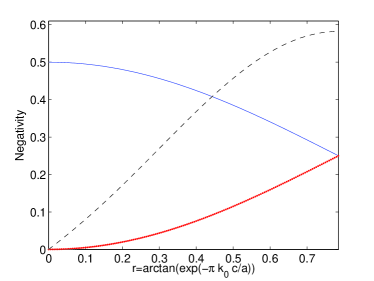
It is remarkable –and constitutes one of the most suggestive results of this article– that we have obtained here a conservation law for the entanglement Alice-Rob and Alice-AntiRob, since the sum of both negativities is independent of the accelerations

𝒩dAR¯+𝒩dAR=12subscriptsuperscript𝒩𝐴¯𝑅𝑑superscriptsubscript𝒩𝑑𝐴𝑅12\mathcal{N}^{A\bar{R}}_{d}+\mathcal{N}_{d}^{AR}=\frac{1}{2} (51)

This is similar to the result (42) for mutual information. Again, one could check that for spinless fermion fields the same conservation law (51) obtained here applies. This was again expected due to the universality principle demonstrated in Martín-Martínez and León (2009).

As we will see below, this conservation of quantum correlations is exclusive of fermionic fields. Statistics can be blamed for this neat result. This is in line with what was suggested in Martín-Martínez and León (2009), since nothing of the sort will be found for bosonic fields.

IV.2.3 Bipartition Rob-AntiRob

The eigenvalues of the partial transpose density matrix for the bipartition Rob-AntiRob (46) turn out to be

λ1subscript𝜆1\displaystyle\lambda_{1} =\displaystyle= cos4rd2;λ2=sin4rd2superscript4subscript𝑟𝑑2subscript𝜆2superscript4subscript𝑟𝑑2\displaystyle\frac{\cos^{4}r_{d}}{2};\qquad\lambda_{2}=\frac{\sin^{4}r_{d}}{2}
λ3subscript𝜆3\displaystyle\lambda_{3} =\displaystyle= λ4=sin2rdcos2rd2subscript𝜆4superscript2subscript𝑟𝑑superscript2subscript𝑟𝑑2\displaystyle\lambda_{4}=\frac{\sin^{2}r_{d}\cos^{2}r_{d}}{2}
λ5,6subscript𝜆56\displaystyle\lambda_{5,6} =\displaystyle= ±sinrdcos3rd2plus-or-minussubscript𝑟𝑑superscript3subscript𝑟𝑑2\displaystyle\pm\frac{\sin r_{d}\,\cos^{3}r_{d}}{2}
λ7,8subscript𝜆78\displaystyle\lambda_{7,8} =\displaystyle= ±cosrdsin3rd2plus-or-minussubscript𝑟𝑑superscript3subscript𝑟𝑑2\displaystyle\pm\frac{\cos r_{d}\,\sin^{3}r_{d}}{2}
λ9,10subscript𝜆910\displaystyle\lambda_{9,10} =\displaystyle= cos2rd4(1±1+sin2(2rd))superscript2subscript𝑟𝑑4plus-or-minus11superscript22subscript𝑟𝑑\displaystyle\frac{\cos^{2}r_{d}}{4}\left(1\pm\sqrt{1+\sin^{2}(2r_{d})}\right)
λ11,12subscript𝜆1112\displaystyle\lambda_{11,12} =\displaystyle= sin2rd4(1±1+sin2(2rd))superscript2subscript𝑟𝑑4plus-or-minus11superscript22subscript𝑟𝑑\displaystyle\frac{\sin^{2}r_{d}}{4}\left(1\pm\sqrt{1+\sin^{2}(2r_{d})}\right)
λ13,14,15,16subscript𝜆13141516\displaystyle\lambda_{13,14,15,16} =\displaystyle= ±sin(2rd)8(1±1+sin2(2rd))plus-or-minus2subscript𝑟𝑑8plus-or-minus11superscript22subscript𝑟𝑑\displaystyle\pm\frac{\sin(2r_{d})}{8}\left(1\pm\sqrt{1+\sin^{2}(2r_{d})}\right) (52)

and therefore, the sum of the negative eigenvalues gives a negativity

𝒩dRR¯=14[sin(2rd)21+[1+sin(2rd)]1+sin2(2rd)]subscriptsuperscript𝒩𝑅¯𝑅𝑑14delimited-[]2subscript𝑟𝑑21delimited-[]12subscript𝑟𝑑1superscript22subscript𝑟𝑑\mathcal{N}^{R\bar{R}}_{d}=\frac{1}{4}\left[\frac{\sin(2r_{d})}{2}-1+[1+\sin(2r_{d})]\sqrt{1+\sin^{2}(2r_{d})}\right] (53)

As it can be seen from (53) and graphically in fig. 3, the entanglement between Rob and AntiRob, created as Rob accelerates, grows up to a finite value. Although this entanglement is useless for quantum information tasks because of the impossibility of classical communication between both sides of an event horizon, the result obtained here is a useful hint in order to understand how information behaves in the proximity of horizons.

Comparing again this result with spinless fermions Alsing et al. (2006), we see that for Dirac fields, the maximum value of the negativity is greater. Again this is strongly related with the dimension of the Hilbert space, as we will comment more deeply below, when we deal with scalar fields.
Refer to caption
Figure 2: (Colour online) Dirac field: Mutual information tradeoff and conservation law between the systems Alice-Rob and Alice-AntiRob as acceleration varies. It is also shown the behaviour of the mutual information for the system Rob-AntiRob. Blue continuous line: Mutual information AR𝐴𝑅AR, red dotted line: Mutual information AR¯𝐴¯𝑅A\bar{R}, black dashed line: Mutual information RR¯𝑅¯𝑅R\bar{R}
Refer to caption
Figure 3: (Colour online) Dirac field: Negativity tradeoff and conservation law between the systems Alice-Rob and Alice-AntiRob as acceleration varies. It is also shown the behaviour of the quantum correlations for the system Rob-AntiRob. Blue continuous line: Negativity AR𝐴𝑅AR, red dotted line: Negativity AR¯𝐴¯𝑅A\bar{R}, black dashed line: Negativity RR¯𝑅¯𝑅R\bar{R}

V Correlations for the scalar field

The density matrix for the whole tripartite state, which includes modes in both sides of the horizon along with Minkowskian modes, is built from (18)

ρsARR¯=|ΨsΨs|subscriptsuperscript𝜌𝐴𝑅¯𝑅𝑠ketsubscriptΨ𝑠brasubscriptΨ𝑠\rho^{AR\bar{R}}_{s}=\left|{\Psi_{s}}\right\rangle\!\left\langle{\Psi_{s}}\right| (54)

As in the fermion case, the three different bipartitions for the scalar field case are obtained as follows

ρsARsubscriptsuperscript𝜌𝐴𝑅𝑠\displaystyle\rho^{AR}_{s} =\displaystyle= TrIVρsARR¯subscriptTr𝐼𝑉subscriptsuperscript𝜌𝐴𝑅¯𝑅𝑠\displaystyle\operatorname{Tr}_{IV}\rho^{AR\bar{R}}_{s} (55)
ρsAR¯subscriptsuperscript𝜌𝐴¯𝑅𝑠\displaystyle\rho^{A\bar{R}}_{s} =\displaystyle= TrIρsARR¯subscriptTr𝐼subscriptsuperscript𝜌𝐴𝑅¯𝑅𝑠\displaystyle\operatorname{Tr}_{I}\rho^{AR\bar{R}}_{s} (56)
ρsRR¯subscriptsuperscript𝜌𝑅¯𝑅𝑠\displaystyle\rho^{R\bar{R}}_{s} =\displaystyle= TrMρsARR¯subscriptTr𝑀subscriptsuperscript𝜌𝐴𝑅¯𝑅𝑠\displaystyle\operatorname{Tr}_{M}\rho^{AR\bar{R}}_{s} (57)

and the density matrix for each individual subsystem

ρsAsubscriptsuperscript𝜌𝐴𝑠\displaystyle\rho^{A}_{s} =\displaystyle= TrIρsAR=TrIVρsAR¯subscriptTr𝐼subscriptsuperscript𝜌𝐴𝑅𝑠subscriptTr𝐼𝑉subscriptsuperscript𝜌𝐴¯𝑅𝑠\displaystyle\operatorname{Tr}_{I}\rho^{AR}_{s}=\operatorname{Tr}_{IV}\rho^{A\bar{R}}_{s} (58)
ρsRsubscriptsuperscript𝜌𝑅𝑠\displaystyle\rho^{R}_{s} =\displaystyle= TrIVρsRR¯=TrMρsARsubscriptTr𝐼𝑉subscriptsuperscript𝜌𝑅¯𝑅𝑠subscriptTr𝑀subscriptsuperscript𝜌𝐴𝑅𝑠\displaystyle\operatorname{Tr}_{IV}\rho^{R\bar{R}}_{s}=\operatorname{Tr}_{M}\rho^{AR}_{s} (59)
ρsR¯subscriptsuperscript𝜌¯𝑅𝑠\displaystyle\rho^{\bar{R}}_{s} =\displaystyle= TrIρsRR¯=TrMρsAR¯subscriptTr𝐼subscriptsuperscript𝜌𝑅¯𝑅𝑠subscriptTr𝑀subscriptsuperscript𝜌𝐴¯𝑅𝑠\displaystyle\operatorname{Tr}_{I}\rho^{R\bar{R}}_{s}=\operatorname{Tr}_{M}\rho^{A\bar{R}}_{s} (60)

The bipartite systems are characterized by the following density matrices

ρsARsubscriptsuperscript𝜌𝐴𝑅𝑠\displaystyle\rho^{AR}_{s} =\displaystyle= n=0tanh2nrs2cosh2rs[|0n0n|+n+1coshrs(|0n1n+1|\displaystyle\sum_{n=0}^{\infty}\frac{\tanh^{2n}r_{s}}{2\cosh^{2}r_{s}}\Big{[}\left|{0n}\right\rangle\!\left\langle{0n}\right|+\frac{\sqrt{n+1}}{\cosh r_{s}}\Big{(}\left|{0n}\right\rangle\!\left\langle{1\,n+1}\right|
+|1n+10n|)+n+1cosh2rs|1n+11n+1|]\displaystyle+\left|{1\,n+1}\right\rangle\!\left\langle{0n}\right|\Big{)}+\frac{n+1}{\cosh^{2}r_{s}}\left|{1\,n+1}\right\rangle\!\left\langle{1\,n+1}\right|\Big{]}
ρsAR¯subscriptsuperscript𝜌𝐴¯𝑅𝑠\displaystyle\rho^{A\bar{R}}_{s} =\displaystyle\!\!\!=\!\!\! n=0tanh2nrs2cosh2rs[|0n0n|+n+1coshrstanhrs(|0n+1\displaystyle\sum_{n=0}^{\infty}\frac{\tanh^{2n}r_{s}}{2\cosh^{2}r_{s}}\Big{[}\!\left|{0n}\right\rangle\!\left\langle{0n}\right|\!+\!\frac{\sqrt{n+1}}{\cosh r_{s}}\tanh r_{s}\Big{(}\!\left|{0\,n+1}\right\rangle (62)
×1n|+|1n0n+1|)+n+1cosh2rs|1n1n|]\displaystyle\times\left\langle{1n}\right|+\left|{1n}\right\rangle\!\left\langle{0\,n+1}\right|\Big{)}+\frac{n+1}{\cosh^{2}r_{s}}\left|{1n}\right\rangle\!\left\langle{1n}\right|\Big{]}
ρsRR¯subscriptsuperscript𝜌𝑅¯𝑅𝑠\displaystyle\rho^{R\bar{R}}_{s} =\displaystyle= n=0m=0tanhn+mrs2cosh2rs(|nnmm|+n+1m+1cosh2rs\displaystyle\sum_{\begin{subarray}{c}n=0\\ m=0\end{subarray}}^{\infty}\frac{\tanh^{n+m}r_{s}}{2\cosh^{2}r_{s}}\Big{(}\left|{nn}\right\rangle\!\left\langle{mm}\right|+\frac{\sqrt{n+1}\sqrt{m+1}}{\cosh^{2}r_{s}} (63)
×|n+1nm+1m|)\displaystyle\times\left|{n+1\,n}\right\rangle\!\left\langle{m+1\,m}\right|\!\Big{)}

where the bases are respectively

|nmket𝑛𝑚\displaystyle\left|{nm}\right\rangle =\displaystyle= |nAM|mRIsubscriptketsuperscript𝑛𝐴𝑀subscriptketsuperscript𝑚𝑅𝐼\displaystyle\left|{n^{A}}\right\rangle_{M}\left|{m^{R}}\right\rangle_{I} (64)
|nmket𝑛𝑚\displaystyle\left|{nm}\right\rangle =\displaystyle= |nAM|mR¯IVsubscriptketsuperscript𝑛𝐴𝑀subscriptketsuperscript𝑚¯𝑅𝐼𝑉\displaystyle\left|{n^{A}}\right\rangle_{M}|m^{\bar{R}}\rangle_{IV} (65)
|nmket𝑛𝑚\displaystyle\left|{nm}\right\rangle =\displaystyle= |nRI|mR¯IVsubscriptketsuperscript𝑛𝑅𝐼subscriptketsuperscript𝑚¯𝑅𝐼𝑉\displaystyle\left|{n^{R}}\right\rangle_{I}|m^{\bar{R}}\rangle_{IV} (66)

for (V), (62) and (63).

On the other hand, the density matrices for the individual subsystems (58), (59),(60) are

ρsR=n=0tanh2(n1)rs2cosh2rs[tanh2rs+ncosh2rs]|nn|subscriptsuperscript𝜌𝑅𝑠superscriptsubscript𝑛0superscript2𝑛1subscript𝑟𝑠2superscript2subscript𝑟𝑠delimited-[]superscript2subscript𝑟𝑠𝑛superscript2subscript𝑟𝑠ket𝑛bra𝑛\rho^{R}_{s}=\sum_{n=0}^{\infty}\frac{\tanh^{2(n-1)}r_{s}}{2\cosh^{2}r_{s}}\left[\tanh^{2}r_{s}+\frac{n}{\cosh^{2}r_{s}}\right]\left|{n}\right\rangle\!\left\langle{n}\right| (67)
ρsR¯=n=0tanh2nrs2cosh2rs[1+n+1cosh2rs]|nn|subscriptsuperscript𝜌¯𝑅𝑠superscriptsubscript𝑛0superscript2𝑛subscript𝑟𝑠2superscript2subscript𝑟𝑠delimited-[]1𝑛1superscript2subscript𝑟𝑠ket𝑛bra𝑛\rho^{\bar{R}}_{s}=\sum_{n=0}^{\infty}\frac{\tanh^{2n}r_{s}}{2\cosh^{2}r_{s}}\left[1+\frac{n+1}{\cosh^{2}r_{s}}\right]\left|{n}\right\rangle\!\left\langle{n}\right| (68)
ρsA=12(|00|+|11|)subscriptsuperscript𝜌𝐴𝑠12ket0bra0ket1bra1\rho^{A}_{s}=\frac{1}{2}\left(\left|{0}\right\rangle\!\left\langle{0}\right|+\left|{1}\right\rangle\!\left\langle{1}\right|\right) (69)

V.1 Mutual Information: creation, exchange and conservation

Mutual information accounts for correlations (both quantum and classical) between two different parts of the system. Its definition is (36).

To compute the mutual information for each bipartition we will need the eigenvalues of the corresponding density matrices. We shall go through all the process detailedly in the lines below.

V.1.1 Bipartition Alice-Rob

The density matrix for the system Alice-Rob (V) consists on an infinite number of 2×2222\times 2 blocks in the basis {|0n,|1n+1}n=0superscriptsubscriptket0𝑛ket1𝑛1𝑛0\{\left|{0n}\right\rangle,\left|{1\,n+1}\right\rangle\}_{n=0}^{\infty} which have the form

tanh2nrs2cosh2rs(1n+1coshrsn+1coshrsn+1cosh2rs)superscript2𝑛subscript𝑟𝑠2superscript2subscript𝑟𝑠1𝑛1subscript𝑟𝑠𝑛1subscript𝑟𝑠𝑛1superscript2subscript𝑟𝑠\frac{\tanh^{2n}r_{s}}{2\cosh^{2}r_{s}}\left(\!\begin{array}[]{cc}1&\dfrac{\sqrt{n+1}}{\cosh r_{s}}\\ \dfrac{\sqrt{n+1}}{\cosh r_{s}}&\dfrac{n+1}{\cosh^{2}r_{s}}\end{array}\!\right) (70)

whose eigenvalues are

λn1subscriptsuperscript𝜆1𝑛\displaystyle\lambda^{1}_{n} =\displaystyle= 00\displaystyle 0
λn2subscriptsuperscript𝜆2𝑛\displaystyle\lambda^{2}_{n} =\displaystyle= tanh2nrs2cosh2rs(1+n+1cosh2rs)superscript2𝑛subscript𝑟𝑠2superscript2subscript𝑟𝑠1𝑛1superscript2subscript𝑟𝑠\displaystyle\frac{\tanh^{2n}r_{s}}{2\cosh^{2}r_{s}}\left(1+\frac{n+1}{\cosh^{2}r_{s}}\right) (71)

V.1.2 Bipartition Alice-AntiRob

Excepting the diagonal element corresponding to |0000|ket00bra00\left|{00}\right\rangle\!\left\langle{00}\right| (which forms a 1×1111\times 1 block itself) the density matrix for the system Alice-AntiRob (62) consists on an infinite number of 2×2222\times 2 blocks in the basis {|0n,|1n1}n=1superscriptsubscriptket0𝑛ket1𝑛1𝑛1\{\left|{0n}\right\rangle,\left|{1\,n-1}\right\rangle\}_{n=1}^{\infty} which have the form

tanh2nrs2cosh2rs(1nsinhrsnsinhrsnsinh2rs)superscript2𝑛subscript𝑟𝑠2superscript2subscript𝑟𝑠1𝑛subscript𝑟𝑠𝑛subscript𝑟𝑠𝑛superscript2subscript𝑟𝑠\frac{\tanh^{2n}r_{s}}{2\cosh^{2}r_{s}}\left(\!\begin{array}[]{cc}1&\dfrac{\sqrt{n}}{\sinh r_{s}}\\ \dfrac{\sqrt{n}}{\sinh r_{s}}&\dfrac{n}{\sinh^{2}r_{s}}\\ \end{array}\!\right) (72)

We can gather all the eigenvalues in the following expression

λn1subscriptsuperscript𝜆1𝑛\displaystyle\lambda^{1}_{n} =\displaystyle= tanh2nrs2cosh2rs(1+nsinh2rs)superscript2𝑛subscript𝑟𝑠2superscript2subscript𝑟𝑠1𝑛superscript2subscript𝑟𝑠\displaystyle\frac{\tanh^{2n}r_{s}}{2\cosh^{2}r_{s}}\left(1+\frac{n}{\sinh^{2}r_{s}}\right)
λn2subscriptsuperscript𝜆2𝑛\displaystyle\lambda^{2}_{n} =\displaystyle= 00\displaystyle 0

V.1.3 Bipartition Rob-AntiRob

It is easy to see that the density matrix for Rob-AntiRob (63) –which basically consists in the direct sum of two blocks of infinite dimension– only has range rank(ρsRR¯)=2ranksubscriptsuperscript𝜌𝑅¯𝑅𝑠2\operatorname{rank}(\rho^{R\bar{R}}_{s})=2. Therefore its eigenvalues are zero except for two of them, which are

λ1RR¯subscriptsuperscript𝜆𝑅¯𝑅1\displaystyle\lambda^{R\bar{R}}_{1} =\displaystyle= n=0tanh2nrs2cosh2rs=12superscriptsubscript𝑛0superscript2𝑛subscript𝑟𝑠2superscript2subscript𝑟𝑠12\displaystyle\sum_{n=0}^{\infty}\frac{\tanh^{2n}r_{s}}{2\cosh^{2}r_{s}}=\frac{1}{2}
λ2RR¯subscriptsuperscript𝜆𝑅¯𝑅2\displaystyle\lambda^{R\bar{R}}_{2} =\displaystyle= n=0(n+1)tanh2nrs2cosh4rs=12superscriptsubscript𝑛0𝑛1superscript2𝑛subscript𝑟𝑠2superscript4subscript𝑟𝑠12\displaystyle\sum_{n=0}^{\infty}\frac{(n+1)\tanh^{2n}r_{s}}{2\cosh^{4}r_{s}}=\frac{1}{2} (74)

So, the Von Neumann entropy for ρRR¯superscript𝜌𝑅¯𝑅\rho^{R\bar{R}} is

SRR¯=1superscript𝑆𝑅¯𝑅1S^{R\bar{R}}=1 (75)

V.1.4 Von Neumann entropies for each subsystem and mutual information

To compute the Von Neumann entropies we need the eigenvalues of every bipartition and the individual density matrices. The eigenvalues of ρsARsubscriptsuperscript𝜌𝐴𝑅𝑠\rho^{AR}_{s}, ρsAR¯subscriptsuperscript𝜌𝐴¯𝑅𝑠\rho^{A\bar{R}}_{s}, ρsRR¯subscriptsuperscript𝜌𝑅¯𝑅𝑠\rho^{R\bar{R}}_{s} are respectively (V.1.1), (V.1.2) and (V.1.3).

The eigevalues of the individual systems density matrices can be directly read from (67), (68) and (69) since ρsRsubscriptsuperscript𝜌𝑅𝑠\rho^{R}_{s}, ρsR¯subscriptsuperscript𝜌¯𝑅𝑠\rho^{\bar{R}}_{s} and ρsAsubscriptsuperscript𝜌𝐴𝑠\rho^{A}_{s} have diagonal forms in the Fock basis. The Von Neumann entropy for a partition B𝐵B of the system is (40).

At this point, computing the entropies is quite straightforward. Von Neumann entropy for the Rob partial system is

SRsubscript𝑆𝑅\displaystyle S_{R} =\displaystyle= n=0tanh2(n1)rs2cosh2rs(tanh2rs+ncosh2rs)superscriptsubscript𝑛0superscript2𝑛1subscript𝑟𝑠2superscript2subscript𝑟𝑠superscript2subscript𝑟𝑠𝑛superscript2subscript𝑟𝑠\displaystyle-\sum_{n=0}^{\infty}\frac{\tanh^{2(n-1)}r_{s}}{2\cosh^{2}r_{s}}\Big{(}\tanh^{2}r_{s}+\frac{n}{\cosh^{2}r_{s}}\Big{)} (76)
×log2[tanh2(n1)rs2cosh2rs(tanh2rs+ncosh2rs)]absentsubscript2superscript2𝑛1subscript𝑟𝑠2superscript2subscript𝑟𝑠superscript2subscript𝑟𝑠𝑛superscript2subscript𝑟𝑠\displaystyle\!\!\!\!\!\!\!\times\log_{2}\!\left[\frac{\tanh^{2(n-1)}r_{s}}{2\cosh^{2}r_{s}}\Big{(}\tanh^{2}r_{s}+\frac{n}{\cosh^{2}r_{s}}\Big{)}\!\right]

The partial matrices have a similar mathematical structure. Therefore, we can express the non-trivial entropies for the all the possible partitions as a function of the entropy (76) for Rob’s partial system

SR¯subscript𝑆¯𝑅\displaystyle S_{\bar{R}} =\displaystyle= SRtanh2rs12sinh2rslog2(12cosh2rs)subscript𝑆𝑅superscript2subscript𝑟𝑠12superscript2subscript𝑟𝑠subscript212superscript2subscript𝑟𝑠\displaystyle\frac{S_{R}}{\tanh^{2}r_{s}}-\frac{1}{2\sinh^{2}r_{s}}\log_{2}\left(\frac{1}{2\cosh^{2}r_{s}}\right)
+log2(tanh2rs)subscript2superscript2subscript𝑟𝑠\displaystyle+\log_{2}\Big{(}\tanh^{2}r_{s}\Big{)}
SARsubscript𝑆𝐴𝑅\displaystyle S_{AR} =\displaystyle= SR¯;SAR¯=SR;SRR¯=SA=1formulae-sequencesubscript𝑆¯𝑅subscript𝑆𝐴¯𝑅subscript𝑆𝑅subscript𝑆𝑅¯𝑅subscript𝑆𝐴1\displaystyle S_{\bar{R}};\qquad\!\!S_{A\bar{R}}=S_{R};\qquad\!\!S_{R\bar{R}}=S_{A}=1 (77)

Notice that the expression for SR¯subscript𝑆¯𝑅S_{\bar{R}} may appear to blow up as rs0subscript𝑟𝑠0r_{s}\rightarrow 0, however this is not the case and it can be checked analytically using (76) that limr0SR¯=0subscript𝑟0subscript𝑆¯𝑅0\lim_{r\rightarrow 0}S_{\bar{R}}=0.

The mutual information for all the possible bipartitions of the system will be

IARsubscript𝐼𝐴𝑅\displaystyle I_{AR} =\displaystyle= SA+SRSAR=1+SRSR¯subscript𝑆𝐴subscript𝑆𝑅subscript𝑆𝐴𝑅1subscript𝑆𝑅subscript𝑆¯𝑅\displaystyle S_{A}+S_{R}-S_{AR}=1+S_{R}-S_{\bar{R}}
IAR¯subscript𝐼𝐴¯𝑅\displaystyle I_{A\bar{R}} =\displaystyle= SA+SRSAR¯=1+SR¯SRsubscript𝑆𝐴subscript𝑆𝑅subscript𝑆𝐴¯𝑅1subscript𝑆¯𝑅subscript𝑆𝑅\displaystyle S_{A}+S_{R}-S_{A\bar{R}}=1+S_{\bar{R}}-S_{R}
IRR¯subscript𝐼𝑅¯𝑅\displaystyle I_{R\bar{R}} =\displaystyle= SR+SR¯SRR¯=SR+SR¯1subscript𝑆𝑅subscript𝑆¯𝑅subscript𝑆𝑅¯𝑅subscript𝑆𝑅subscript𝑆¯𝑅1\displaystyle S_{R}+S_{\bar{R}}-S_{R\bar{R}}=S_{R}+S_{\bar{R}}-1

Again we obtain a conservation law of the mutual information for the system Alice-Rob and Alice-AntiRob

IAR+IAR¯=2subscript𝐼𝐴𝑅subscript𝐼𝐴¯𝑅2I_{AR}+I_{A\bar{R}}=2 (78)

which again suggests a correlations transfer from the system Alice-Rob to Alice-AntiRob as the acceleration increases.

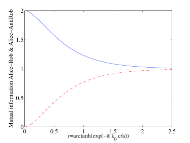
Although the conservation law is the same as for fermion fields (42), the specific dependance of the mutual information with the acceleration is different, as it can be seen in fig. 4. Later, when we analyse the negativity for all the bipartitions, we will see that, even though mutual information fulfills this conservation law, we must wait for the analysis of quantum correlations to appreciate the striking differences between fermions and bosons.

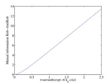
Fig.5 shows how the correlations across the horizon (Rob and AntiRob) increase with no bound as Rob accelerates. This unbounded growing is not only strongly related with the infinite dimension of the Hilbert space, but also very much influenced by statistics. As we will see later, we require the infinite dimension of the bosons Hilbert space in order to have correlations RR¯𝑅¯𝑅R\bar{R} which survive the limit a𝑎a\rightarrow\infty. That is not the case for fermions, where those correlations survive the limit even though the Hilbert space has finite dimension. We will discuss how the infinite dimension is responsible for the unbounded growing of correlations across the horizon after studying the negativity in subsection V.2.
Refer to caption
Figure 4: (Colour online) Scalar field: Mutual information tradeoff and conservation law between the systems Alice-Rob and Alice-AntiRob. Blue continuous line: Mutual information AR𝐴𝑅AR, red dashed line: Mutual information AR¯𝐴¯𝑅A\bar{R}, red dashed line: Mutual information AR¯𝐴¯𝑅A\bar{R}
Refer to caption
Figure 5: (Colour online) Scalar field: Behaviour of the mutual information for the system Rob-AntiRob as acceleration varies

V.2 Entanglement behaviour across the horizon

As we did above, we will compute the negativity (43) for the scalar case. To compute it, we need the partial transpose of the bipartite density matrices (V), (62) and (63), which we will notate as ηsARsubscriptsuperscript𝜂𝐴𝑅𝑠\eta^{AR}_{s}, ηsAR¯subscriptsuperscript𝜂𝐴¯𝑅𝑠\eta^{A\bar{R}}_{s} and ηsRR¯subscriptsuperscript𝜂𝑅¯𝑅𝑠\eta^{R\bar{R}}_{s} respectively.

ηsARsubscriptsuperscript𝜂𝐴𝑅𝑠\displaystyle\eta^{AR}_{s} =\displaystyle= n=0tanh2nrs2cosh2rs[|0n0n|+n+1coshrs(|0n+11n|\displaystyle\sum_{n=0}^{\infty}\frac{\tanh^{2n}r_{s}}{2\cosh^{2}r_{s}}\Big{[}\left|{0n}\right\rangle\!\left\langle{0n}\right|+\frac{\sqrt{n+1}}{\cosh r_{s}}\Big{(}\left|{0\,n+1}\right\rangle\!\left\langle{1n}\right| (79)
+|1n0n+1|)+n+1cosh2rs|1n+11n+1|]\displaystyle\!\!\!\!\!\!\!+\left|{1n}\right\rangle\!\left\langle{0\,n+1}\right|\Big{)}+\frac{n+1}{\cosh^{2}r_{s}}\left|{1\,n+1}\right\rangle\!\left\langle{1\,n+1}\right|\Big{]}
ηsAR¯subscriptsuperscript𝜂𝐴¯𝑅𝑠\displaystyle\eta^{A\bar{R}}_{s} =\displaystyle\!\!\!=\!\!\! n=0tanh2nrs2cosh2rs[|0n0n|+n+1coshrstanhrs(|0n\displaystyle\sum_{n=0}^{\infty}\frac{\tanh^{2n}r_{s}}{2\cosh^{2}r_{s}}\Big{[}\left|{0n}\right\rangle\!\left\langle{0n}\right|+\frac{\sqrt{n+1}}{\cosh r_{s}}\tanh r_{s}\Big{(}\left|{0n}\right\rangle (80)
×1n+1|+|1n+10n|)+n+1cosh2rs|1n1n|]\displaystyle\!\!\!\!\!\!\times\left\langle{1\,n+1}\right|\!+\!\left|{1\,n+1}\right\rangle\!\left\langle{0n}\right|\!\Big{)}\!+\!\frac{n+1}{\cosh^{2}r_{s}}\left|{1n}\right\rangle\!\left\langle{1n}\right|\!\Big{]}
ηsRR¯subscriptsuperscript𝜂𝑅¯𝑅𝑠\displaystyle\eta^{R\bar{R}}_{s} =\displaystyle= n=0m=0tanhn+mrs2cosh2rs(|nmmn|+n+1m+1cosh2rs\displaystyle\sum_{\begin{subarray}{c}n=0\\ m=0\end{subarray}}^{\infty}\frac{\tanh^{n+m}r_{s}}{2\cosh^{2}r_{s}}\Big{(}\left|{nm}\right\rangle\!\left\langle{mn}\right|+\frac{\sqrt{n+1}\sqrt{m+1}}{\cosh^{2}r_{s}} (81)
×|n+1mm+1n|)\displaystyle\times\left|{n+1\,m}\right\rangle\!\left\langle{m+1\,n}\right|\!\Big{)}

In the following subsections we shall compute the negativity of each bipartition of the system.

V.2.1 Bipartition Alice-Rob

Excepting the diagonal element corresponding to |0000|ket00bra00\left|{00}\right\rangle\!\left\langle{00}\right| (which forms a 1×1111\times 1 block itself), the partial transpose of the density matrix ρsARsubscriptsuperscript𝜌𝐴𝑅𝑠\rho^{AR}_{s} (79) has a 2×2222\times 2 block structure in the basis {|0n+1,|1n}ket0𝑛1ket1𝑛\{\left|{0\,n+1}\right\rangle,\left|{1n}\right\rangle\}

tanh2nrs2cosh2rs(tanh2rsn+1coshrsn+1coshrsnsinh2rs)superscript2𝑛subscript𝑟𝑠2superscript2subscript𝑟𝑠superscript2subscript𝑟𝑠𝑛1subscript𝑟𝑠𝑛1subscript𝑟𝑠𝑛superscript2subscript𝑟𝑠\frac{\tanh^{2n}r_{s}}{2\cosh^{2}r_{s}}\left(\!\begin{array}[]{cc}\tanh^{2}r_{s}&\dfrac{\sqrt{n+1}}{\cosh r_{s}}\\ \dfrac{\sqrt{n+1}}{\cosh r_{s}}&\dfrac{n}{\sinh^{2}r_{s}}\end{array}\!\right) (82)

Hence, the eigenvalues of (79) are

λ1superscript𝜆1\displaystyle\lambda^{1} =\displaystyle= 12cosh2rs12superscript2subscript𝑟𝑠\displaystyle\frac{1}{2\cosh^{2}r_{s}}
λn2subscriptsuperscript𝜆2𝑛\displaystyle\lambda^{2}_{n} =\displaystyle= tanh2nrs4cosh2rs[(nsinh2rs+tanh2rs)\displaystyle\frac{\tanh^{2n}r_{s}}{4\cosh^{2}r_{s}}\left[\left(\frac{n}{\sinh^{2}r_{s}}+\tanh^{2}r_{s}\right)\right. (83)
±(nsinh2rs+tanh2rs)2+4cosh2rs]\displaystyle\left.\pm\sqrt{\left(\frac{n}{\sinh^{2}r_{s}}+\tanh^{2}r_{s}\right)^{2}+\frac{4}{\cosh^{2}r_{s}}}\right]

And then the negativity for this bipartition is

𝒩sARsubscriptsuperscript𝒩𝐴𝑅𝑠\displaystyle\mathcal{N}^{AR}_{s} =\displaystyle= n=0tanh2nrs4cosh2rs|(nsinh2rs+tanh2rs)conditionalsuperscriptsubscript𝑛0superscript2𝑛subscript𝑟𝑠4superscript2subscript𝑟𝑠𝑛superscript2subscript𝑟𝑠superscript2subscript𝑟𝑠\displaystyle\sum_{n=0}^{\infty}\frac{\tanh^{2n}r_{s}}{4\cosh^{2}r_{s}}\left|\left(\frac{n}{\sinh^{2}r_{s}}+\tanh^{2}r_{s}\right)\right. (84)
(nsinh2rs+tanh2rs)2+4cosh2rs|\displaystyle\!\!\!\!\!\!\!\left.-\sqrt{\left(\frac{n}{\sinh^{2}r_{s}}+\tanh^{2}r_{s}\right)^{2}+\frac{4}{\cosh^{2}r_{s}}}\right|

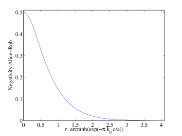
Fig. 6 shows 𝒩sARsubscriptsuperscript𝒩𝐴𝑅𝑠\mathcal{N}^{AR}_{s} as a function of rssubscript𝑟𝑠r_{s}.

Refer to caption
Figure 6: (Colour online) Scalar field: Behaviour of the negativity for the bipartition Alice-Rob as Rob accelerates

V.2.2 Bipartition Alice-AntiRob

Excepting the diagonal element corresponding to |1010|ket10bra10\left|{10}\right\rangle\!\left\langle{10}\right| (which forms a 1×1111\times 1 block itself), the partial transpose of the density matrix ρsAR¯superscriptsubscript𝜌𝑠𝐴¯𝑅\rho_{s}^{A\bar{R}} (80) has a 2×2222\times 2 block structure in the basis {|0n,|1n+1}ket0𝑛ket1𝑛1\{\left|{0n}\right\rangle,\left|{1\,n+1}\right\rangle\}

tanh2nrs2cosh2rs(1tanhrscoshrsn+1tanhrscoshrsn+1tanh2rscosh2rs(n+2))superscript2𝑛subscript𝑟𝑠2superscript2subscript𝑟𝑠1subscript𝑟𝑠subscript𝑟𝑠𝑛1subscript𝑟𝑠subscript𝑟𝑠𝑛1superscript2subscript𝑟𝑠superscript2subscript𝑟𝑠𝑛2\frac{\tanh^{2n}r_{s}}{2\cosh^{2}r_{s}}\left(\!\begin{array}[]{cc}1&\dfrac{\tanh r_{s}}{\cosh r_{s}}\sqrt{n+1}\\ \dfrac{\tanh r_{s}}{\cosh r_{s}}\sqrt{n+1}&\dfrac{\tanh^{2}r_{s}}{\cosh^{2}r_{s}}(n+2)\end{array}\!\right) (85)

Hence, the eigenvalues of (80) are

λ1superscript𝜆1\displaystyle\lambda^{1} =\displaystyle= 12cosh4rs12superscript4subscript𝑟𝑠\displaystyle\frac{1}{2\cosh^{4}r_{s}}
λn2subscriptsuperscript𝜆2𝑛\displaystyle\lambda^{2}_{n} =\displaystyle= tanh2nrs4cosh2rs[(1+(n+2)tanh2rscosh2rs)\displaystyle\frac{\tanh^{2n}r_{s}}{4\cosh^{2}r_{s}}\left[\left(1+(n+2)\frac{\tanh^{2}r_{s}}{\cosh^{2}r_{s}}\right)\right. (86)
±(1+(n+2)tanh2rscosh2rs)24tanh2rscosh2rs]\displaystyle\!\!\!\!\left.\pm\sqrt{\left(1+(n+2)\frac{\tanh^{2}r_{s}}{\cosh^{2}r_{s}}\right)^{2}-\frac{4\tanh^{2}r_{s}}{\cosh^{2}r_{s}}}\right]

Therefore, the negtivity for this bipartition is always 00, independently of the value of Rob’s acceleration. The important implications of this striking result are discussed below.

V.2.3 Bipartition Rob-AntiRob

The partial transpose of the density matrix ρsRR¯subscriptsuperscript𝜌𝑅¯𝑅𝑠\rho^{R\bar{R}}_{s} (81) has a block structure, but the blocks themselves are of different dimensions which grow up to infinity. Because of this, negativity is not as easily computable as for the other cases, not being possible to write it in a closed form.

However it is still possible to compute the eigenvalues of (81) numerically taking into account that the blocks which form the matrix are endomorphisms which act in the subspace expanded by the basis BD={|mn}subscript𝐵𝐷ket𝑚𝑛B_{D}=\{\left|{mn}\right\rangle\} in which m+n=D1=constant𝑚𝑛𝐷1constantm+n=D-1=\text{constant}, which is to say, the fisrt block acts within the subspace expanded by the basis B1={|00}subscript𝐵1ket00B_{1}=\{\left|{00}\right\rangle\}, the second B2={|01,|10}subscript𝐵2ket01ket10B_{2}=\{\left|{01}\right\rangle,\left|{10}\right\rangle\}, the third B3={|02,|20,|11}subscript𝐵3ket02ket20ket11B_{3}=\{\left|{02}\right\rangle,\left|{20}\right\rangle,\left|{11}\right\rangle\}, the fourth B4={|03,|30,|12,|21}subscript𝐵4ket03ket30ket12ket21B_{4}=\{\left|{03}\right\rangle,\left|{30}\right\rangle,\left|{12}\right\rangle,\left|{21}\right\rangle\} and so forth. In this fashion, the whole matrix is an endomorphism within the subspace i=1Sisuperscriptsubscriptdirect-sum𝑖1subscript𝑆𝑖\bigoplus_{i=1}^{\infty}S_{i} being Sisubscript𝑆𝑖S_{i} the subspace (of dimension D=i𝐷𝑖D=i) expanded by the basis Bisubscript𝐵𝑖B_{i}.

Let us denote MDsubscript𝑀𝐷M_{D} the blocks which form the matrix (81), being D𝐷D the dimension of each block. Then its structure is

MD=(0a1000a10a2000a20a3000a30a40000000000aD100000aD1aD)subscript𝑀𝐷0subscript𝑎1000subscript𝑎10subscript𝑎2000subscript𝑎20subscript𝑎3000subscript𝑎30subscript𝑎40000000000subscript𝑎𝐷100000subscript𝑎𝐷1subscript𝑎𝐷M_{D}=\left(\!\begin{array}[]{cccccccc}0&a_{1}&0&0&\cdots&\cdots&\cdots&0\\ a_{1}&0&a_{2}&0&\cdots&\cdots&\cdots&0\\ 0&a_{2}&0&a_{3}&\cdots&\cdots&\cdots&0\\ 0&0&a_{3}&0&a_{4}&\cdots&\cdots&0\\ 0&0&0&\ddots&\ddots&\ddots&\cdots&0\\ \vdots&\vdots&\vdots&\vdots&\ddots&\ddots&\ddots&\vdots\\ 0&0&0&0&\cdots&\ddots&0&a_{D-1}\\ 0&0&0&0&0&\dots&a_{D-1}&a_{D}\\ \end{array}\!\right) (87)

which is to say, the diagonal terms are zero except for the last one, and the rest of the matrix elements are zero excepting the two diagonals on top and underneath the principal diagonal. The elements ansubscript𝑎𝑛a_{n} are defined as follows

a2l+1=(tanhrs)D12cosh2rssubscript𝑎2𝑙1superscriptsubscript𝑟𝑠𝐷12superscript2subscript𝑟𝑠a_{2l+1}=\frac{(\tanh r_{s})^{D-1}}{2\cosh^{2}r_{s}} (88)
a2l=Dll(tanhrs)D22cosh4rssubscript𝑎2𝑙𝐷𝑙𝑙superscriptsubscript𝑟𝑠𝐷22superscript4subscript𝑟𝑠a_{2l}=\sqrt{D-l}\,\sqrt{l}\frac{(\tanh r_{s})^{D-2}}{2\cosh^{4}r_{s}} (89)

Notice that the elements are completely different when the value of the label n𝑛n is odd or even.

As the whole matrix is the direct sum of the blocks

ηsRR¯=D=1MDsuperscriptsubscript𝜂𝑠𝑅¯𝑅superscriptsubscriptdirect-sum𝐷1subscript𝑀𝐷\eta_{s}^{R\bar{R}}=\bigoplus_{D=1}^{\infty}M_{D} (90)

the eigenvalues and, specifically, the negative eigenvalues of ηsRR¯superscriptsubscript𝜂𝑠𝑅¯𝑅\eta_{s}^{R\bar{R}} would be the negative eigenvalues of all the blocks MDsubscript𝑀𝐷M_{D} gathered togheter. It can be shown that the absolute value of the negative eigenvalues of the blocks decreases quickly as the dimension increases. Thus, the negativity 𝒩sRR¯subscriptsuperscript𝒩𝑅¯𝑅𝑠\mathcal{N}^{R\bar{R}}_{s} converges promtply to a finite value for a given value of rssubscript𝑟𝑠r_{s}. Fig 7 shows the behaviour of 𝒩sRR¯subscriptsuperscript𝒩𝑅¯𝑅𝑠\mathcal{N}^{R\bar{R}}_{s} with rssubscript𝑟𝑠r_{s}, showing that the entanglement increases unboundedly between Rob and AntiRob.

Let us compare these results with the fermion case.

First, as it was shown in Alsing et al. (2006), the negativity of the system Alice-Rob decreases as Rob accelerates, vanishing in the limit a𝑎a\rightarrow\infty, instead of remaining finite as in the fermionic cases Alsing et al. (2006); León and Martín-Martínez (2009).

What may be more surprising is the behaviour of quantum correlations of the system Alice-AntiRob. In the fermion case negativity grows monotonically from zero (for a=0𝑎0a=0) to a finite value (for a=𝑎a=\infty). Nevertheless, for scalars, Alice-AntiRob negativity is identically zero for all acceleration. Hence, there is no transfer of entanglement from Alice-Rob to Alice-AntiRob as it was the case for fermions. Still, correlations (classical) are not lost as it can be concluded from (78).

Why do we obtain such loss of entanglement for the bosonic case and, conversely, it does not happen in the fermionic case? The answer is, once again, statistics.

One could think of the infinite dimensionality of the Hilbert space for scalars (compared to the finite dimension for fermions) as the cause of this different behaviour. However we shall prove that it has to do with the bosonic nature of the field rather than with the infinite dimensionality of the Hilbert space. We can see this considering hardcore bosons instead of scalars, which is to say, we can limit the occupation number for the bosonic modes to a certain finite limit N𝑁N instead of taking N𝑁N\rightarrow\infty. By doing so, we transform the infinite dimension Hilbert space for bosons into a finite dimension one. As we will see below, in any case, the negativity would continue being zero for all a𝑎a.

To illustrate this argument, we could compare the fermionic case with the hardcore bosonic case with N=2𝑁2N=2 which would be its analogous, namely, a bosonic field whose occupation number is limited to 222. Looking at the partially transposed density matrix for the fermionic case, we can seek for the negative eigenvalues origin and, then, compare the analogous structure that would appear for the hardcore bosonic case. We will see that, in the latter case, no negative eigenvalues are obtained.

Recalling the form of the matrix (45), we can see that it has a structure of four 1×1111\times 1 blocks, which give positive eigenvalues, and two 2×2222\times 2 blocks, which are the ones whose eigenvalues contribute to the negativity. These two blocks are

12(cos4rdsinrdcos2rdsinrdcos2rd0)12superscript4subscript𝑟𝑑subscript𝑟𝑑superscript2subscript𝑟𝑑subscript𝑟𝑑superscript2subscript𝑟𝑑0\frac{1}{2}\left(\!\begin{array}[]{cc}\cos^{4}r_{d}&\sin r_{d}\cos^{2}r_{d}\\[5.12149pt] \sin r_{d}\cos^{2}r_{d}&0\\ \end{array}\!\right) (91)

in the basis {|00,|}\left\{\left|{00}\right\rangle,\left|{\uparrow\uparrow}\right\rangle\right\} and

12(sin2rdcos2rdsin3rdsin3rd0)12superscript2subscript𝑟𝑑superscript2subscript𝑟𝑑superscript3subscript𝑟𝑑superscript3subscript𝑟𝑑0\frac{1}{2}\left(\!\begin{array}[]{cc}\sin^{2}r_{d}\cos^{2}r_{d}&-\sin^{3}r_{d}\\[5.12149pt] -\sin^{3}r_{d}&0\\ \end{array}\!\right) (92)

in the basis {|0,|p}\left\{\left|{0\downarrow}\right\rangle,\left|{\uparrow p}\right\rangle\right\}.

For hardcore bosons with occupation number limited to n=N𝑛𝑁n=N the structure would be quite similar to (80), but this time we would have two 1×1111\times 1 blocks instead of one (the elements |0000|ket00bra00\left|{00}\right\rangle\!\left\langle{00}\right| and |NNNN|ket𝑁𝑁bra𝑁𝑁\left|{NN}\right\rangle\!\left\langle{NN}\right|) and N𝑁N 2×2222\times 2 blocks with the structure (85) but with n=0,,N1𝑛0𝑁1n=0,\dots,N-1. Specifically, for N=2𝑁2N=2 the two blocks are

12cosh2rs(1tanhrscoshrstanhrscoshrs2tanh2rscosh2rs)12superscript2subscript𝑟𝑠1subscript𝑟𝑠subscript𝑟𝑠subscript𝑟𝑠subscript𝑟𝑠2superscript2subscript𝑟𝑠superscript2subscript𝑟𝑠\frac{1}{2\cosh^{2}r_{s}}\left(\!\begin{array}[]{cc}1&\dfrac{\tanh r_{s}}{\cosh r_{s}}\\[7.11317pt] \dfrac{\tanh r_{s}}{\cosh r_{s}}&\dfrac{2\tanh^{2}r_{s}}{\cosh^{2}r_{s}}\end{array}\!\right) (93)

in the basis {|00,|11}ket00ket11\left\{\left|{00}\right\rangle,\left|{11}\right\rangle\right\} and

tanh2rs2cosh2rs(12tanhrscoshrs2tanhrscoshrs3tanh2rscosh2rs)superscript2subscript𝑟𝑠2superscript2subscript𝑟𝑠12subscript𝑟𝑠subscript𝑟𝑠2subscript𝑟𝑠subscript𝑟𝑠3superscript2subscript𝑟𝑠superscript2subscript𝑟𝑠\frac{\tanh^{2}r_{s}}{2\cosh^{2}r_{s}}\left(\!\begin{array}[]{cc}1&\dfrac{\sqrt{2}\tanh r_{s}}{\cosh r_{s}}\\[7.11317pt] \dfrac{\sqrt{2}\tanh r_{s}}{\cosh r_{s}}&\dfrac{3\tanh^{2}r_{s}}{\cosh^{2}r_{s}}\end{array}\!\right) (94)

in the basis {|01,|12}ket01ket12\left\{\left|{01}\right\rangle,\left|{12}\right\rangle\right\}.

The key difference comes from the second diagonal term of the blocks, which in the fermionic case it is impossible to obtain due to the peculiar structure that fermionic statistics imposes on (III). On the other hand, for bosons this term is non-zero, and furthermore it has a value large enough to prevent the partial transposed density matrix from having negative eigenvalues.

As mentioned in section III, this result is independent of the election of the particular value for the spin components for Alice and Rob in (19). It also does not depend on N𝑁N (the limit for occupation number we impose to hardcore bosons modes) and this phenomenon is exclusively ruled by statistics. Besides, this is an evidence of the difference between hardcore bosons and fermions, which sometimes in the literature are considered as the same. This is not the case, at least speaking about quantum correlations, about which we have observed that statistics is a key feature.

This is additional confirmation of the important role that statistics plays in the behaviour of correlations in non-inertial frames, and specifically in the proximity of black holes. In fact, getting closer and closer to the Rindler horizon (i.e. a𝑎a\rightarrow\infty) the situation resembles more and more the scenario in which Rob is arbitrarily close to the event horizon of a Schwartzschild black hole, while Alice is free-falling into it.

About the bipartition Rob-AntiRob, at first glance at fig 5 and 7 one could think that there might be some inconsistency between the behaviour of entanglement and mutual information, as the latter grows linearly while negativity seems to grow exponentially. Since mutual information accounts for all the correlations (quantum and classical) between Rob and AntiRob, the result may appear paradoxical. However this apparently inconsistent results are due to the fact that negativity cannot be identified as the entanglement itself, but as a monotone which grows as the degree of entanglement does. The specific functional form chosen for the monotone is not imposed by physical motivations. Actually, we could have chosen logarithmic negativity –instead of negativity– as our entanglement monotone since it is in fact better to be compared with mutual information due to its additivity properties Plenio (2005). The result obtained in this case, shown in fig. 8, is that when acceleration grows both growths become linear.

Coming back to the argumental line of this paper, we observe that entanglement grows unboundedly for this bipartition, conversely to the fermion case in which negativity increases up to a certain finite limit as Rob accelerates. This different behaviour is related not only with the dimension of the Hilbert space but also it is strongly influenced by statistics.

Actually, if we consider again hardcore bosons we can see from (87) that limiting the dimension would give a finite number of blocks which contribute to the negativity, being the last one truncated and having dimension N1𝑁1N-1 instead of N+1𝑁1N+1. In any case, taking the limit a𝑎a\rightarrow\infty we can see that negative eigenvalues of the partially transpose density matrix tend to zero as a𝑎a grows. Therefore negativity vanishes in that limit.

Naturally, the same happened in the standard bosonic case, but then we had that negativity was the sum of an infinite number of terms each vanishing when a𝑎a\rightarrow\infty. The negativity resulted divergent, although. Now we are adding only a finite number of vanishing terms so that negativity, which was divergent when a𝑎a\rightarrow\infty for standard bosons, now vanishes in such limit. This behaviour contrasts with the fermionic case and the standard scalar field case.

This and other points related with the impact of dimension and statistics on this correlations across the horizon will appear elsewhere.
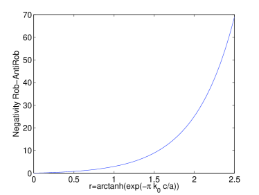
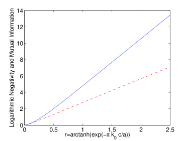
Refer to caption
Figure 7: (Colour online) Scalar field: Behaviour of the negativity for the bipartition Rob-AntiRob as Rob accelerates
Refer to caption
Figure 8: (Colour online) Scalar field: Comparison of growth of quantum and all (quantum+classical) correlations for the system Rob-AntiRob as acceleration increases. Quantum correlations are accounted for by logarithmic negativity. This figure compares this entanglement measurement with mutual information. Blue continuous line represents mutual information and red dashed line represents Logarithmic negativity

VI Conclusions

This work focused on the bipartite correlations between different spatial-temporal domains in the presence of an event horizon. Specifically, we analyse all the possible bipartitions of an entangled system composed by an inertial observer and an accelerated one, who inhabits a universe with an event horizon.

As pointed out in the introduction, Rindler space-time is the simplest case which, presenting a horizon, also reproduces two interesting physical scenarios. Namely, it describes the point of view of an uniformly accelerated observer and, in the limit a𝑎a\rightarrow\infty, it reproduces an observer resisting arbitrarily close to a Swchartzschild black hole event horizon.

First of all, we have studied the relation between the behaviour of entanglement of the system Alice-Rob and Alice-AntiRob, which are the two bipartitions to which one could assign physical meaning. We have shown that the dimension of the Hilbert space has little to do with the entanglement behaviour.

We recall two results to support this statement, on one hand, in Martín-Martínez and León (2009) we studied the case of a Dirac and a spinless fermion field beyond the single mode approximation in which fermionic Hilbert space turned out to have infinite dimension. On the other hand, here we have analysed bosons in a Hilbert space of infinite and finite dimensions (scalar field and hardcore scalar respectively). The results are that the characteristic differences between fermion fields and bosonic fields for the bipartitions AR𝐴𝑅AR and AR¯𝐴¯𝑅A\bar{R} manifest independently of the dimension of the Hilbert space.

Here we have disclosed a great difference in the behaviour of quantum correlations for fermions and bosons. In the fermionic case we showed that, at the same time as Unruh decoherence destroys the entanglement of the system Alice-Rob, entanglement is created between Alice and AntiRob. This means that the quantum entanglement lost between Alice and the field modes outside the event horizon is gained between Alice and the modes inside. This is expressed through the entanglement conservation law (51), which we have deduced for fermions.

Nevertheless, for bosonic states it was shown that, as acceleration increases, entanglement is quickly and completely lost between Alice and Rob while no quantum correlations are created between Alice and AntiRob. Moreover, no entanglement of any kind survives among any physical bipartition of the system in the limit a𝑎a\rightarrow\infty for the bosonic case. This contrasts with the fermionic case where the amount of entanglement among all the physical bipartitions of the system remains always constant.

This goes in the line of the previous work Martín-Martínez and León (2009) in which we suggested that all the entanglement which survives a black hole event horizon is purely statistical, and gives no further information than the statistical correlations which inescapably appear due to the fermionic nature of the field.

These powerful and suggesting results may well be related with what was obtained in previous works as Schliemann et al. (2001); Ghirardi and Marinatto (2004). In those works it was demonstrated, for pure states in first quantization, that the fact of considering indistinguishable fermions implies that there are quantum correlations of which we cannot get rid due to the antisymmetrisation of the fermionic wavefunctions. Of course, the scenario here is not the same, but analysing together the results obtained here and those in Schliemann et al. (2001); Ghirardi and Marinatto (2004) reveals the somewhat special feature of fermionic fields regarding entanglement comportment: statistics information, or in this case, information of the fermionic nature of the field, cannot be erased from our system, and still, that information is expressed by means of quantum correlations.

Another remarkable result is the conservation law for mutual information for fermions (42) and bosons (78) shown in in fig. 2 and fig. 4. The detailed behaviour is different for both cases but the same conservation law is obtained for the mutual information of the bipartitions Alice-Rob, and Alice AntiRob. Mutual information accounts for both classical and quantum correlations (despite the fact that in general there is no trivial relation between negativity and mutual information). However for the bosonic case, the mutual information distributes between the systems Alice-Rob and Alice-AntiRob more rapidly than for the fermion case.

This result for mutual information means that correlations are always conserved for the systems Alice-Rob and Alice-AntiRob, despite the fact that quantum correlations vanish for the bosonic case and they are preserved (and this is the effect of statistics) in the fermionic case. The fact that classical correlations behave in a similar way for fermions and bosons while quantum correlations comport so differently suggests again that the quantum entanglement which survives the black hole limit is merely statistical.

Another difference between fermion and bosons appears analysing the correlations between modes inside and outside the horizon. It is interesting to notice that, as the non-inertial partner accelerates, correlations across the horizon are created. Both, dimension of the Hilbert space and statistics, play a fundamental role in the behaviour of these correlations. We have obtained that for Dirac fields these correlations, quantum and classical, grow as Rob accelerates up to a finite value at the limit a𝑎a\rightarrow\infty. This limit is greater than the analogous limit obtained for spinless fermions in Alsing et al. (2006) whose Hilbert space for each mode is smaller. For the bosonic case, on the contrary, those correlations grow unboundedly, being infinite when a𝑎a\rightarrow\infty. Surprisingly, for the hardcore bosonic field, in which Hilbert space have an arbitrarily large but finite dimension, the behaviour of this correlations is not even monotonical, being zero for the inertial limit as well as for the infinite acceleration regime, but non-zero in between. Therefore, statistics and dimensionality must be taken into account in order to find the origin of this comportment.

We have dealt with this bipartition separately since it cannot be given a physical interpretation in terms of information theory. However, it is worthwhile to analyse its comportment since it could reveal the relative roles of dimensionality and statistics when accounting for the behaviour of correlations in the presence of an event horizon. This topic, which deserves further study, is expected to appear elsewhere.

It is important to recall that the limit a𝑎a\rightarrow\infty can be understood as considering an observer moving in a trajectory arbitrarily close to the event horizon of a Schwarzschild black hole Fuentes-Schuller and Mann (2005). So, along with the interest of describing the correlations between accelerated observers, this study gives further insight about the fate of correlations in the presence of a black hole. Together with Martín-Martínez and León (2009), our results could be of use to tackle the problem of the information paradox in black holes, for which they indicate that statistics plays a very important role.

VII Acknowledgments

This work was partially supported by the Spanish MICINN Project FIS2008-05705/FIS and by the CAM research consortium QUITEMAD S2009/ESP-1594. E. M-M was partially supported by a CSIC JAE-PREDOC2007 Grant.

References

  • Alsing and Milburn (2003) P. M. Alsing and G. J. Milburn, Phys. Rev. Lett. 91, 180404 (2003).
  • Terashima and Ueda (2004) H. Terashima and M. Ueda, Phys. Rev. A 69, 032113 (2004).
  • Shi (2004) Y. Shi, Phys. Rev. D 70, 105001 (2004).
  • Fuentes-Schuller and Mann (2005) I. Fuentes-Schuller and R. B. Mann, Phys. Rev. Lett. 95, 120404 (2005).
  • Alsing et al. (2006) P. M. Alsing, I. Fuentes-Schuller, R. B. Mann, and T. E. Tessier, Phys. Rev. A 74, 032326 (2006).
  • Ball et al. (2006) J. L. Ball, I. Fuentes-Schuller, and F. P. Schuller, Phys. Lett. A 359, 550 (2006).
  • Adesso et al. (2007) G. Adesso, I. Fuentes-Schuller, and M. Ericsson, Phys. Rev. A 76, 062112 (2007).
  • Brádler (2007) K. Brádler, Phys. Rev. A 75, 022311 (2007).
  • Ling et al. (2007) Y. Ling, S. He, W. Qiu, and H. Zhang, J. of Phys. A 40, 9025 (2007).
  • Ahn et al. (2008) D. Ahn, Y. Moon, R. Mann, and I. Fuentes-Schuller, J. High Energy Phys. 2008, 062 (2008).
  • Pan and Jing (2008) Q. Pan and J. Jing, Phys. Rev. D 78, 065015 (2008).
  • Alsing et al. (2004) P. M. Alsing, D. McMahon, and G. J. Milburn, J. Opt. B: Quantum Semiclass. Opt. 6, S834 (2004).
  • Doukas and Hollenberg (2009) J. Doukas and L. C. L. Hollenberg, Phys. Rev. A 79, 052109 (2009).
  • Steeg and Menicucci (2009) G. Steeg and N. C. Menicucci, Phys. Rev. D 79, 044027 (2009).
  • León and Martín-Martínez (2009) J. León and E. Martín-Martínez, Phys. Rev. A 80, 012314 (2009).
  • Adesso and Fuentes-Schuller (2009) G. Adesso and I. Fuentes-Schuller, Quant. Inf. Comput. 9, 0657 (2009).
  • Davies (1975) P. C. W. Davies, J. of Phys. A 8, 609 (1975).
  • Unruh (1976) W. G. Unruh, Phys. Rev. D 14, 870 (1976).
  • Takagi (1986) S. Takagi, Prog. Theor. Phys. Suppl. 88, 1 (1986).
  • Crispino et al. (2008) L. C. B. Crispino, A. Higuchi, and G. E. A. Matsas, Rev. Mod. Phys. 80, 787 (2008).
  • Martín-Martínez and León (2009) E. Martín-Martínez and J. León, Phys. Rev. A 80, 042318 (2009).
  • Misner et al. (1973) C. W. Misner, K. S. Thorne, and J. A. Wheeler, Gravitation (W. H. Freeman, 1973).
  • Birrell and Davies (1984) N. D. Birrell and P. C. W. Davies, Quantum Fields in Curved Space (Cambridge University Press, 1984).
  • Jáuregui et al. (1991) R. Jáuregui, M. Torres, and S. Hacyan, Phys. Rev. D 43, 3979 (1991).
  • Plenio (2005) M. B. Plenio, Phys. Rev. Lett. 95, 090503 (2005).
  • Schliemann et al. (2001) J. Schliemann, J. I. Cirac, M. Kus, M. Lewenstein, and D. Loss, Phys. Rev. A 64, 022303 (2001).
  • Ghirardi and Marinatto (2004) G. C. Ghirardi and L. Marinatto, Phys. Rev. A 70, 012109 (2004).