Network of Recurrent events - A case study of Japan

Abstract

A recently proposed method of constructing seismic networks from “record breaking events” from the earthquake catalog of California (Phy. Rev. E, 77 6,066104, 2008) was successfull in establishing causal features to seismicity and arrive at estimates for rupture length and its scaling with magnitude. The results of our implementation of this procedure on the earthquake catalog of Japan establishes the robustness of the procedure. Additionally, we find that the temporal distributions are able to detect heterogeneties in the seismicity of the region.

I Introduction

Earthquakes are a prime example of a natural phenomenon– where the spatial and temporal coordinates of an event can be measured with a fair degree of accuracy even as the dynamics of the process is not fully understood. The unpredictability of an earthquake occurence has not been reduced by more numerous or more accurate measurements. The difficulties of seismic analysis involves understanding the roles of the static/geometrical heterogeneities in fault zones, the dynamic heterogeneities that result as stress builds up in the moving lithospheric plates and the possible interactions between the two BS2004 . The multidimensional character of seismicity makes it difficult to model it and this is further hampered by the restrictions of having to apply our understanding of rock friction from lab based results to the enormous length and time scales associated with earthquakes. In order to develop a realistic model for seismicity and for assessing the seismic potential of a region, the factors mentioned above needs to be estimated correctly. This will involve being able to measure the stress and strain at all points along the active fault - which is currently impossible  Jdetal2006 .

The observed clustering of earthquakes suggests that events are correlated in space-time. Thus, studies of earthquake correlations are important for understanding the dynamics of the process and for evolving prediction algorithms. In recent times, a large body of work in seismic studies involves relating the topology of complex networks constructed from earthquake catalogs of a region to the spatio-temporal patterns exhibited by seismicity there. Such an approach is based on the idea that the patterns of seismicity may shed light on the fundamental physics, since these patterns are the emergent processes of the underlying many body nonlinear systemJdetal2006 . New patterns in the clustering of seismicity in space and time, new parameters that characterise the seismicity in a region, causal connections between subsequent events, novel methods to estimate the rupture length and its scaling with magnitude – are some of the prominent outcomes of these catalog based studies ( see for eg. AbeSuz2004 ; BaPcz2004 ; BaPcz2005 ; Eisneretal2005 ; AbeSuz2006 ; AbeSuz2006-2 ; Ba2006 ; Grassetal2007 ). The central idea contained in these studies is to treat all events in the catalog on the same footing. That is, the space - time window based distinctions of events as foreshocks - mainshocks - aftershocks is avoided. Causal connections are extended to beyond immediately subsequent events and also an event can have more than one correlated predecessor. In these studies, correlations between events have been established from different perspectives and complex networks are constructed by linking correlated events. For example, the region studied may be divided into small cubic cells. Each cell becomes a node in the network if an event happens within it. The network is linked by directed edges between nodes representing successive events in the catalog AbeSuz2004 ; AbeSuz2006 ; AbeSuz2006-2 . Alternately, correlations have been quantified with a metric which incorporates the fractal dimension $d_{f}$ and the $b$ value of the catalog used. Links are made between highly correlated events with directed edges BaPcz2004 ; BaPcz2005 ; Ba2006 .

A third procedure involves identifying record breaking recurrences of an event and linking each event in the catalog to its recurrences with directed edges Jdetal2006 ; Grassetal2007 . This procedure, illustrated on the earthquake catalog of Southern California had evolved a general method for inferring causal connections. The patterns exhibited by a network constructed from the actual catalog of the region was compared with the network of a randomly shuffled catalog (acausal) in order to establish causal features. In addition, this approach provides a method of estimating the rupture length, its scaling with magnitude and in identifying new scaling laws associated with the seismicity of the region.

In this paper, we apply the procedure developed by the authorsJdetal2006 ; Grassetal2007 on the earthquake catalog of Japan, in order to study the patterns exhibited by its network and to examine the robustness of the procedure for different seismic regions. This paper is organised as follows:- Section II briefly describes the construction of the network, Section III will describe the catalogs used for the analysis, Section IV contains the results and a discussion of it and in Section V we conclude.

II Construction of the network

The procedure described in Grassetal2007 is followed here to identify the recurrences and to construct the network. A directed network is constructed by linking each event $i$, (i = 1,2,3,$\cdots$ ,N) in a catalog of $N$ events with a magnitude threshold of $m_{th}$, with an edge pointing from it ( main event) to its recurrence. Each recurrence $j$, ( j = i+1,$\cdots$ ,N) is a record breaking event which is closer to the main event $i$ than any event $k$ in the intervening period $t_{j}-t_{i}$ where $t_{j}>t_{k}>t_{i}$. This implies that the $(i+1)^{th}$ event is the first recurrence of the $i^{th}$ event for $i=1,2,\cdots,N-1$ and is always a recurrence however distant it might be. In this way, each event gets to have its own list of recurrences which follow it in time. This definition of a recurrence is based solely on the spatiotemporal relations between events in the catalog and has no arbitrariness in its selection. Also, any event identified as a recurrence of a main event does not loose its status if the period of the catalog is enlarged later, as this will only result in the list of recurrences getting longer if the added events satisfy the condition of coming closer to the main event in the intervening period. The network is constructed by considering every event in the catalog as a node and each recurrence is represented by a directed edge between the pair of events, directed according to the time ordering of the earthquakes. The two variables associated with each edge are – $l_{ij}$, the distance between the epicentres of the two events and $t_{ij}$, the time interval between the them. Each node has an out-degree equal to its number of outward edges (the number of its recurrences) and an in-degree equal to the number of events it is counted to be a recurrence of. The first event in the catalog will not have any incoming edges to it and the last event in the catalog will have no outgoing edges from it. Note that the recurrences defined here do not necessarily relate to the conventional methods of defining aftershocks and thus the largest magnitude event in the network need not have the most number of recurrences. The overall structure of the network represented by the outgoing links and the incoming links describes the clustering of seismicity in the region studied.

III The Catalog

The catalog studied here is the Japan University Network Earthquake Catalog jap_catalog covering the rectangular region $(126.433^{\circ}\mathrm{E}$–$148.0^{\circ}\mathrm{E})$ longitude and $(25.730^{\circ}\mathrm{N}$–$47.831^{\circ}\mathrm{N})$ latitude, for the period between January, 1986–December, 1998. The catalog has a threshold magnitude of $m_{JMA}$ =$2.0$. However, we have limited our study to events with magnitude  $\geq 2.5$. The total number of such events are $114804$. In order to verify the dependance of the network properties on magnitude threshold and on the number of events, subsets with higher magnitude thresholds viz   $3.0$, $3.5$, $4.0$ and $4.5$ which contain $53525$, $20067$, $6268$ and $2038$ events respectively and a subcatalog with $m_{th}$  = 3.0 for a shorter period from 1986 –1992 with 22975 events, were generated from the main catalog. The $b$ value = $-0.87$ was obtained from a plot of $\log N(m)$ vs $m$, where $N(m)$ is the cumulative number of earthquakes of magnitudes $\geq m$, and the linear fit was good in the range $2.5\leq m\leq 7$. In order to distinguish the causal features of seismicity, networks were constructed from the shuffled catalog, where we have adopted an identical shuffling procedure as in Grassetal2007 . Subsets and sub catalogs of the shuffled catalog are also made for the same $m_{th}$ values as for the actual catalog. We propose to contrast the features of their in/out-degree, recurrent length and recurrent time distributions in order to relate the features of the seismic network of Japan with that of California Grassetal2007 .

Figure 1: A spatial plot of the earthquake catalog jap_catalog with $m_{th}$ =2.5 for the period 1986 -1998. The catalog contains 114804 events.

IV Results

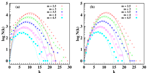
Figure 2: The panels (a) and (b) in the figure represent the degree distributions for the actual and the shuffled catalogs respectively. The points represent the out-degree and lines of the same colour as the points represent the corressponding in-degree distributions for the different $m_{th}$ values shown in the legend of the graph. The in-degree, for all $m_{th}$ values is almost a Poisson distribution for both the actual and the shuffled catalogs. The out-degree of the actual catalog shows significant deviations from Poisson behaviour for low and higher degree values. In case of the shuffled catalog, the marginal deviation from Poisson behaviour is only towards the higher degree values.

IV.1 Degree distributions

The in-degree and out-degree of every node in each of the networks of different $m_{th}$ is estimated and the histograms in Fig. 2(a) show the degree distributions for the actual catalog. The points and the lines of the same colour represent the out-degree and the in-degree distributions respectively, for each $m_{th}$ value. As observed for California Grassetal2007 , the in-degree histograms are all Poisson in nature while the out-degrees show an excess of nodes with lesser and higher degree when compared to a Poisson distribution of the same mean degree. The panel $(b)$ in Fig. 2 represents the in/out-degree histograms for the shuffled catalog which is equivalent to random process. The in-degree for the shuffled catalog is observed to be a Poisson distribution. In a random network, the out-degree distributions are also expected to be Poisson. The shuffled catalog has an out-degree which though not a typical Poisson distribution, shows significant differences when compared to the out-degree distributions of the actual network especially for the lower degree values. For each network, the mean in-degree is equal to the mean out-degree. As expected, this decreases with $m_{th}$  because the number of nodes and therefore, the number of links decrease with $m_{th}$. For a Poisson distribution, it is expected that $\langle k\rangle\approx\log N$, which is what we observe in Fig. 3 for the shuffled catalog. For the actual catalog however, the number of links are less than that of a random network and we get $\langle k\rangle\approx 0.91\log N$. The value $0.91$ is higher than that reported for California in  Grassetal2007 and this means that larger number of links are possible for the nodes in the Japanese seismic network.

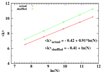
Figure 3: The plot shows the variation of the mean degree, $\langle k\rangle$ with the number of events $N$. The lines represent the best fits from which the slope ie estimated. The shuffled catalog, which is equivalent to a random process, shows a slope $=1$ while the actual catalog shows a lower value of $\approx$ 0.91.

IV.2 Distance distributions

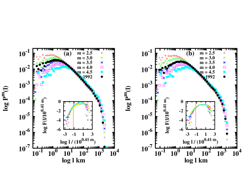
Figure 4: The figure shows the distribution of the distances of recurrences for the different magnitude thresholds. The panel marked $(a)$ is for the actual catalog and the one marked $(b)$ for the shuffled catalog. The black points in both the plots represent a smaller catalog(1986 -1992) with $m_{th}$ = 3.0. For the actual catalog, the size of the catalog does not affect the position of the peak as seen in the peak positions of the green and black points. However, for the shuffled catalog, the distance distribution varies with size of the catalog. The inset shows the data collapse achieved by rescaling the distances and the distributions according to eqn. 1. The red line in the inset represents the pre-factor $L_{o}$ in the scaling law for the rupture length given by $l^{\ast}(m)=L_{o}\times 10^{0.41m_{th}}$, where $L_{o}$ = 0.066 km

We use the great circle distance for computing the distance  $l_{ij}$  between two event locations. This is calculated using the Haversine formula haversine : if $(\phi_{i},\lambda_{i})$ and $(\phi_{j},\lambda_{j})$ are the (latitude, longitude) values for the two event locations and, $\Delta\phi=\phi_{j}-\phi_{i}$ and $\Delta\lambda=\lambda_{i}-\lambda_{j}$, then

$$l_{ij}=R\Delta\sigma$$

where $\Delta\sigma$, the spherical distance, or central angle, between the two event locations is

$$\Delta\sigma=2\arcsin\left(\sqrt{\sin^{2}\left(\frac{\Delta\phi}{2}\right)+\cos(\phi_{i})\cos(\phi_{j})\sin^{2}\left(\frac{\Delta\lambda}{2}\right)}\right).$$

$R$, the radius of the earth, is taken as $6367~{}km$. The PDF of the recurrent distances for all the $i-j$ recurrent pairs in the actual network is shown in a $\log-\log$ plot of $P_{m}(l)$ versus $l$ in Fig. 4(a). The different coloured points are for networks with different $m_{th}$values. All the plots show that the PDF is unimodal and exhibits a peak at a typical distance $l^{\ast}_{m}$. The position of the peak is invariant with respect to the length of the catalog as can be seen from the peak positions of the green and black points, which corresspond to different catalog sizes having the same $m_{th}$ value of $3.0$. Though we have not shown it in the figure, we have verified this for the other $m_{th}$ values also. The peak position however, depends upon $m_{th}$ and increases with it. Beyond the peak the distribution shows a power law decrease with an exponent $\approx 1.2$ upto a cut-off which represents the size of the region studied. Since the least count of the catalog for latitude and longitude values is $0.001^{o}$, which translates to a least measurable distance $\approx 0.1$km, we are unable to resolve the points at distances $<$ 100mts. This affects the unnambiguous recognition of the peak for the lower $m_{th}$ plots. The position of the peaks for each plot ($l^{\ast}_{m}$) was estimated by fitting a quadratic near the region of the peak. The variation of $l^{\ast}_{m}$ with $m$ was studied to arrive at the rescaling parameter of $0.41$ for the inset data collapse in Fig. 4(a). The data collapse obeys the relation

$$P^{m}(l)\approx l^{-1.2}F(l/10^{0.41m_{th}})$$ (1)

The scaling function $F$ has two regimes– a power law increase with an exponent $\approx 1.8$ for small arguments and a constant regime at larger arguments. The characteristic distance of the peaks can be written as

$$l^{*}(m)=L_{o}\times 10^{0.41m_{th}}$$ (2)

where $L_{o}=0.066$. The distance distributions for the shuffled catalog in Fig. 4(b) shows the same overall shape as for the actual catalog. We also find that the peaks shift to higher values of $l$ as $m_{th}$ increases. However, one important variation observed here was that the position of the peak is not independant of $N$. This striking and important feature was reported for the California catalog too Grassetal2007 . The invariance of $l^{\ast}_{m}$ for the actual catalog was attributed to the causal structure of seismicity and is therefore expected to reflect the features of the underlying dynamics Grassetal2007 .

IV.2.1 Identifcation with rupture length

An useful outcome of constructing such a network of recurrent events is, being able to arrive at an estimate for the rupture length in the region, from its earthquake catalog. The values of $l^{\ast}_{m}$ are identified as the rupture lengths and in the case of the California region the values obtained were reported to be in good agreement with the estimates given in Kagan2002 ; Wells1994 . The identification of $l^{\ast}_{m}$ as the rupture length is further established by the appearance of the same distances in the distribution of the distances of the first recurrences. The distribution of the first recurrences for California had the form

$$P_{1}^{m}(l)=l^{-\delta_{r}}\bar{F}(l/10^{0.45m_{th}})$$ (3)

with $\delta_{r}=0.6$. The first recurrence of an event $i$ is the distance between the $i^{th}$ and $(i+1)^{th}$ event. The distances of the first recurrence is estimated for all the events in the catalog and its distribution for the actual catalog is shown in fig.5. We also observe the peaks for the different $m_{th}$ values appearing at the same distances as in fig. 4 and therefore the $l^{\ast}_{m}$ values estimated from fig. 4 can be considered as the rupture lengths as indicated in Grassetal2007 . The distribution of first recurrences in our analysis can be written as

$$P_{1}^{m}(l)=l^{-\delta_{r}}\bar{F}(l/10^{0.41m_{th}})$$ (4)

with $\delta_{r}=0.6$ and the scaling function $\bar{F}$ has the same form as $F$ in fig. 4.

The rupture lengths for Japan estimated using eqn. 2 compares favourably with the values estimated using $L_{R}(m^{\prime})\approx 0.02\times 10^{0.5m{{}^{\prime}}}$  Kagan2002 and $L_{R}(m^{\prime})\approx 0.018\times 10^{0.46m{{}^{\prime}}}$  Wells1994 as seen from Table 1

Table 1: The values tabulated here show a comparison of the rupture lengths estimated by this procedure with other estimates in Kagan2002 ; Wells1994 . Note that the magnitude scale used in  Kagan2002 ; Wells1994 are moment magnitude ($M_{w}$). We have used the relation $M_{w}=0.58M_{JMA}+2.25$  Scord2005 in order to convert the JMA magnitude values to its equivalent moment magnitude.

$M_{JMA}$	$M_{w}$	$=0.02\times 10^{0.5m{{}^{\prime}}}$km	$=0.018\times 10^{0.46m{{}^{\prime}}}$km	= $0.066\times 10^{0.41m_{th}}$km
3.0	3.99	1.97	1.23	1.12
3.5	4.28	2.76	1.67	1.79
4.0	4.57	3.85	2.27	2.88
4.5	4.86	5.38	3.09	4.61

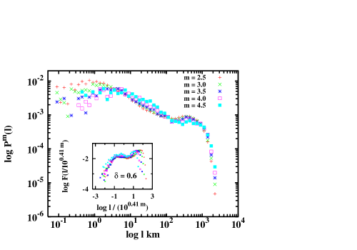
Figure 5: The distribution of distances of the first recurrence for the different $m_{th}$ values is shown here. The peaks at the characteristic distances that was observed in fig. 4 is visible here too. The inset shows the datacollpase achieved by rescaling the distances and the distributions according to eqn. 4.

IV.3 Temporal distribution of recurrences

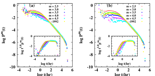
Figure 6: The distributions of the recurrent times for different $m_{th}$ values is shown here in panels $(a)$ and $(b)$ for the actual and shuffled catalogs respectively. Significant differences can be observed between the two distributions. However, the dependence of the distributions on $m$ in the actual catalog is , a major departure from what is expected from a causal network Grassetal2007 .

The PDF of the time intervals $t_{ij}$, between events and their recurrences for different $m_{th}$ values is shown in a $\log-\log$ plot in fig. 6(a) for the actual catalog and in the panel marked (b) for the shuffled catalog. As observed for the California region, for intermediate times the distributions show a power law decay with an exponent $\approx 1.0$ with an observational cut-off at the longest time scales. The distributions for the different $m_{th}$ values are all collapsed showing no dependance on magnitude in this region. However, in the region of the shorter time scales, the different distributions show a dependance on $m$. The power law exponent in this region is much less than $1.0$ and varies from $-0.3$ to $-0.45$ as $m_{th}$ increases from $2.5$ to $4.5$. The range over which this smaller exponent holds good depends on $m_{th}$ and increases with it. This aspect of the recurrent time distributions is at variance with that observed for California, where the temporal distributions were found to be independent of $m$ for the actual catalog and showed a single power law regime over almost the entire range. This behaviour was attributed to the causal features of seismicity. The recurrent time distributions for the shuffled catalog in fig. 6(b) shows a more prominent dependence on $m$, which is expected for a random network Grassetal2007 . That the actual catalog for Japan too shows characteristics attributed to an acausal network signifies a random behaviour in the temporal distributions in the case of Japan.

V Conclusions

The general procedure that was introduced to infer causal structure from clusters of localised events was illustrated on the earthquake catalog of California. Our results from adopting the procedure on the earthquake catalog of Japan confirms its robustness. The construction of the network involves establishing correlations between nodes without making any assumptions regarding the nature of the correlations. The distinctive features of the seismic network when compared to an acausal network was attributed to the causal connections between events. Our results show that features of random networks are universal with the shuffled catalogs of both the regions showing identical network properties. The network from the actual catalog on the other hand shows some region specific features along with exhibiting typical causal attributes. The estimates of rupture length which arise as natural outcomes of the network construction are in good agreement with values estimated by other methods. The anamolies that are shown by the recurrent time distributions in the case of Japan when compared to expectations for a causal network could be a result of the heterogenous nature of seismicity in the region. Japan experiences a high level of seismicity due to its position at the cusp of the Pacific-Philippine-Eurasian triple plate junction. It has a predominantly compressional tectonic regime as compared to Western United States which is dominantly extensional Brodsky2006 . We expect this aspect, along with the fact that different recurrence intervals exist in Japan for earthquakes in subduction zones as compared to areas along crustal faults, to influence the recurrent time distributions which is shown in our results here. However analysis of catalogs for other such regions would have to be done in order to confirm this stand.

References

- [1] Bruce E. Shaw. Dynamic heterogenieties versus fixed heterogeneities in earthquake models. Geophys. J. Int., 156:275–286, 2004.
- [2] J. Davidsen, P. Grassberger, and M. Paczuski. Earthquake recurrence as a record breaking process. GeoPhy. Res. Lett., 33(L11304), 2006.
- [3] S. Abe and N. Suzuki. Scale–free network of earthquakes. Europhysics Letters, 65(4):581–586, 2004.
- [4] M. Baiesi and M. Paczuski. Scale-free networks of earthquakes and aftershocks. Phy. Rev.E, 69(066106), 2004.
- [5] M. Baiesi and M. Paczuski. Complex networks of earthquakes and aftershocks. Nonlinear Processes in Geophysics, 12:1–11, 2005.
- [6] L. Eisner, S. Arrowsmith, J. Le Calvez, and J. Rutledge. Graph Theory for Seismic Analyses. AGU Spring Meeting Abstracts, pages A1+, May 2005.
- [7] S. Abe and N. Suzuki. Complex-network description of seismicity. Nonlinear Processes in Geophysics, (13):145–150, 2006.
- [8] S. Abe and N. Suzuki. Complex earthquake networks: Heirarchial organisation and assortative mixing. Physical Review E, 74:026113–5, 2006.
- [9] Marco Baiesi. Scaling and precursor motifs in earthquake networks. Physica A, (360):534–542, 2006.
- [10] J. Davidsen, P. Grassberger, and M. Paczuski. Networks of recurrent events, a theory of records and an application to finding causal signatures in seismicity. Phy. Rev. E, 77(6):066104, 2008.
- [11] http://kea.eri.u-tokyo.ac.jp/catalog/junec/monthly.html.
- [12] R. W. Sinnott. Virtues of the haversine. Sky and Telescope, 68(2):159, 1984.
- [13] Y. Y. Kagan. Bulletin of the Seismological Society of America, 92:641, 2002.
- [14] D.L. Wells and K.J. Coppersmith. Bulletin of the Seismological Society of America, 84(4):974, 1994.
- [15] E. M. Scordilis. Globally valid relations converting Ms, mb and MJMA to Mw. in Book of Abstracts of NATO Advanced Research Work-shop, Earthquake Monitoring and Seismic Hazard Mitigation in Balkan Countries (Borovetz, Bulgaria, September 11–-17, 2005).
- [16] Rebecca M. Harrington and Emily E. Brodsky. The Absence of Remotely Triggered Seismicity in Japan. Bulletin of the Seismological Society of America, 96(3):871–878, 2006.