Time-dependent quantum transport in a resonant tunnel junction coupled to a nanomechanical oscillator

Abstract

We present a theoretical study of time-dependent quantum transport in a resonant tunnel junction coupled to a nanomechanical oscillator within the non-equilibrium Green’s function technique. An arbitrary voltage is applied to the tunnel junction and electrons in the leads are considered to be at zero temperature. The transient and the steady state behavior of the system is considered here in order to explore the quantum dynamics of the oscillator as a function of time. The properties of the phonon distribution of the nanomechnical oscillator strongly coupled to the electrons on the dot are investigated using a non-perturbative approach. We consider both the energy transferred from the electrons to the oscillator and the Fano factor as a function of time. We discuss the quantum dynamics of the nanomechanical oscillator in terms of pure and mixed states. We have found a significant difference between a quantum and a classical oscillator. In particular, the energy of a classical oscillator will always be dissipated by the electrons whereas the quantum oscillator remains in an excited state. This will provide useful insight for the design of experiments aimed at studying the quantum behavior of an oscillator.

I Introduction

Nanoscopic physics has been a subject of increasing experimental and theoretical interest for its potential applications in nanoelectromechanical systems (NEMS)1 ; 2 ; 3 . The physical properties of these devices are of crucial importance in improving our understanding of the fundamental science in this area including many-body phenomena4 . One of the most striking paradigms exhibiting many body effects in mesoscopic science is quantum transport through single electronic levels in quantum dots and single molecules5 ; 6 ; 7 ; 8 coupled to external leads. Realizations of these systems have been obtained using semiconductor beams coupled to single electron transistors (SET’s) and superconducting single electron transistors (SSET’s)9 ; 10 , carbon nanotubes11 and, most recently, suspended graphene sheets12 . Such systems can be used as a direct measure of small displacements, forces and mass in the quantum regime. The quantum transport properties of these systems require extremely sensitive measurement that can be achieved by using SET’s, or a resonant tunnel junction, and SSET’s. In this context, NEMS are not only interesting devices studied for ultrasensitive transducers but also because they are expected to exhibit several exclusive features of transport phenomena such as avalanche-like transport and shuttling instability13 ; 14 . The nanomechanical properties of a resonant tunnel junction coupled to an oscillator15 or a SET16 ; 17 coupled to an oscillator are currently playing a vital role in enhancing the understanding of NEMS.

The nanomechanical oscillator coupled to a resonant tunnel junction or SET is a close analogue of a molecule being used as a sensor whose sensitivity has reached the quantum limit1 ; 2 ; 3 ; 9 ; 18 . The signature of quantum states has been predicted for the nanomechanical oscillator coupled to the SET’s9 and SSET’s10 ; 19 . In these experiments, it has been confirmed that the nanomechanical oscillator is strongly affected by the electron transport in the circumstances where we are also trying to explore the quantum regime of NEMS. In this system, electrons tunnel from one of the leads to the isolated conductor and then to the other lead. Phonon assisted tunneling of non–resonant systems has mostly been shown by experiments on inelastic tunneling spectroscopy (ITS). With the advancement of modern technology, as compared to ITS, scanning tunneling spectroscopy (STS) and scanning tunneling microscopy (STM) have proved more valuable tools for the investigation and characterization of molecular systems20 in the conduction regime. In STS experiments, significant signatures of the strong electron-phonon interaction have been observed21 ; 22 beyond the established perturbation theory. Hence, a theory beyond master equation approach or linear response is necessary. Most of the theoretical work on transport in NEMS has been done within the scattering theory approach (Landauer) but it disregards the contacts and their effects on the scattering channel as well as effect of electrons and phonons on each other23 . Very recently, the non–equilibrium Green’s function (NEGF) approach24 ; 25 ; 26 has been growing in importance in the quantum transport of nanomechanical systems15 ; 16 ; 17 ; 18 ; 27 ; 28 . An advantage of this method is that it treats the infinitely extended reservoirs in an exact way29 , which may lead to a better understanding of the essential features of NEMS. NEGF has been applied in the study of shot noise in chain models30 and disordered junctions31 while noise in Coulomb blockade Josephson junctions has been discussed within a phase correlation theory approach32 . In the case of an inelastic resonant tunneling structure, in which strong electron-phonon coupling is often considered, a very strong source-drain voltage is expected for which coherent electron transport in molecular devices has been considered by some workers33 within the scattering theory approach. Inelastic effects on the transport properties have been studied in connection with NEMS and substantial work on this issue has been done, again within the scattering theory approach23 . Recently, phonon assisted resonant tunneling conductance has been discussed within the NEGF technique at zero temperature34 . To the best of our knowledge, in all these studies, time-dependent quantum transport properties of a resonant tunnel junction coupled to a nanomechanical oscillator have not been discussed so far. The development of time-dependent quantum transport for the treatment of nonequilibrium system with phononic as well as Fermionic degree of freedom has remained a challenge since the 1980’s35 . Generally, time-dependent transport properties of mesoscopic systems without nanomechanical oscillator have been reported36 and, in particular, sudden joining of the leads with quantum dot molecule have been investigated35 ; 37 for the case of a noninteracting quantum dot and for a weakly Coulomb interacting molecular system. Strongly interacting systems in the Kondo regime have been investigated38 ; 39 . More recently40 , the transient effects occurring in a molecular quantum dot described by an Anderson-Holstein Hamiltonian has been discussed. To this end, we present the following study.

In the present work, we shall investigate the time evolution of a quantum dot coupled to a single vibrational mode as a reaction to a sudden joining to the leads. We employ the non-equilibrium Green’s function method in order to discuss the transient and steady state dynamics of NEMS. This is a fully quantum mechanical formulation whose basic approximations are very transparent, as the technique has already been used to study transport properties in a wide range of systems. In our calculation inclusion of the oscillator is not perturbative as the STS experiments21 ; 22 are beyond the perturbation theory. So a non-perturbative approach is required beyond the quantum master equation27 ; 28 ; 41 or linear response. Hence, our work provides an exact analytical solution to the current–voltage characteristics, including coupling of leads with the system, very small chemical potential difference and both the right and left Fermi level response regimes. For simplicity, we use the wide-band approximation25 ; 35 ; 42 ; 43 , where the density of states in the leads and hence the coupling between the leads and the dot is taken to be independent of energy. Although the method we are using does not rely on this approximation. This provides a way to perform transient transport calculations from first principles while retaining the essential physics of the electronic structure of the dot and the leads. Another advantage of this method is that it treats the infinitely extended reservoirs in an exact way in the present system, which may give a better understanding of the essential features of NEMS in a more appropriate quantum mechanical picture.

II Model calculations

We consider a single quantum dot connected to two identical metallic leads. A single oscillator is coupled to the electrons on the dot and the applied gate voltage is used to tune the single level of the dot. In the present system, we neglect the spin degree of freedom and electron-electron interaction effects and consider the simplest possible model system. We also neglect the effects of finite electron temperature of the lead reservoirs and damping of the oscillator. Our model consists of the individual entities such as the single quantum dot and the left and right leads in their ground states at zero temperature. The Hamiltonian of our simple system34 ; 42 ; 43 is

$$H_{\mbox{\scriptsize dot-ph}}=\left[\epsilon_{0}+\lambda l(b^{\dagger}+b)\right]c_{0}^{{\dagger}}c_{0}+\hbar\omega(b^{\dagger}b+{\mathchoice{{\textstyle{\frac{1}{2}}}}{{\textstyle{\frac{1}{2}}}}{{\scriptstyle{1/2}}}{{\scriptscriptstyle{1/2}}}})\,,$$ (1)

where $\epsilon_{0}$ is the single energy level of electrons on the dot with $c_{0}^{{\dagger}},c_{0}$ the corresponding creation and annihilation operators, the coupling strength, $\eta=\lambda l,$ with $\lambda=eE,$ is the electrostatic field between electrons on the dot and an oscillator, seen by the electrons due to the charge on the oscillator, $l=\sqrt{\hbar/2m\omega}$ is the zero point amplitude of the oscillator, $\omega$ is the frequency of the oscillator and $b^{\dagger},b$ are the raising and lowering operator of the phonons. The remaining elements of the Hamiltonian are

$$H_{\mbox{\scriptsize leads}} = \sum_{j}\epsilon_{j}c_{j}^{\dagger}c_{j},$$ (2)

$$H_{\mbox{\scriptsize leads-dot}} = \frac{1}{\sqrt{N}}\sum_{j}V_{\alpha}(t)\left(c_{j}^{\dagger}c_{0}+c_{0}^{\dagger}c_{j}\right),$$ (3)

where we include time-dependent hopping $V_{\alpha}(t)$ to enable us to connect the leads $\alpha=L,R$ to the dot at a finite time. For the time-dependent dynamics, we shall focus on sudden joining of the leads to the dot at $t=0$, which means $V_{\alpha}(t)=V\theta(t)$, where $\theta(t)$ is the Heaviside unit step function. $N$ is the total number of states in the lead, and $j$ represents the channels in one of the leads. For the second lead the Hamiltonian can be written in the same way. The total Hamiltonian of the system is thus $H=H_{\mbox{\scriptsize dot-ph}}+H_{\mbox{\scriptsize leads}}+H_{\mbox{\scriptsize leads-dot}}\,$. We write the eigenfunctions of $H_{\mbox{\scriptsize dot-ph}}$ as

$$\Psi_{m}(K,x_{0}\neq 0) = A_{m}\exp[-{\textstyle\frac{l^{2}K^{2}}{2}}]\operatorname{H}_{m}(lK)\exp[-\mathrm{i}Kx_{0}]$$ (4)

$$\Psi_{n}(K,x_{0}=0) = A_{n}\exp[-{\textstyle\frac{l^{2}K^{2}}{2}}]\operatorname{H}_{n}(lK)\,,$$ (5)

for the occupied, $x_{0}\not=0$ and unoccupied, $x_{0}=0$, dot respectively, where $x_{0}={\lambda}/{2m\omega^{2}}$ is the shift of the oscillator due to the coupling to the electrons on the dot, where $A_{n}={1}/{\sqrt{\sqrt{\pi}2^{n}n!l}}$, $A_{m}={1}/{\sqrt{\sqrt{\pi}2^{m}m!l}}$, and $\operatorname{H}_{n}(lK)$ are the usual Hermite polynomials. Here we have used the fact that the harmonic oscillator eigenfunctions have the same form in both real and Fourier space ($K$).

In order to transform between the representations for the occupied and unoccupied dot we require the matrix with elements $\Phi_{nm}=\int\Psi_{n}^{\ast}(K,x_{0}=0)\Psi_{m}(K,x_{0}\neq 0)\,{\mathrm{d}}K,$ which may be simplified44 as

$$\Phi_{n,m} = \frac{l}{\sqrt{\pi 2^{m+n}n!m!}}\int\exp\left(-l^{2}K^{2}\right)\operatorname{H}_{n}^{\ast}(lK)\operatorname{H}_{m}(lK)\exp\left(\mathrm{i}Kx_{0}\right)\,{\mathrm{d}}K$$ (6)

$$= \sqrt{\frac{2^{m-n}n!}{m!}}\exp\left(-{\textstyle\frac{1}{4}}x^{2}\right)\left({\mathchoice{{\textstyle{\frac{1}{2}}}}{{\textstyle{\frac{1}{2}}}}{{\scriptstyle{1/2}}}{{\scriptscriptstyle{1/2}}}}\mathrm{i}x\right)^{m-n}\operatorname{L}_{n}^{m-n}\left({\mathchoice{{\textstyle{\frac{1}{2}}}}{{\textstyle{\frac{1}{2}}}}{{\scriptstyle{1/2}}}{{\scriptscriptstyle{1/2}}}}{x^{2}}\right)$$ (7)

for $n\leq m$, where $x={x_{0}}/{l}$ and $\operatorname{L}_{n}^{m-n}(x)$ are the associated Laguerre polynomials. Note that the integrand is symmetric in $m$ and $n$ but the integral is only valid for $n\leq m$. Clearly the result for $n>m$ is obtained by exchanging $m$ and $n$ in equation (7) to obtain

$$\Phi_{n,m}=\sqrt{\frac{2^{|m-n|}\min[n,m]!}{\max[n,m]!}}\exp\left(-\textstyle\frac{1}{4}x^{2}\right)\left(\mathchoice{{\textstyle{\frac{1}{2}}}}{{\textstyle{\frac{1}{2}}}}{{\scriptstyle{1/2}}}{{\scriptscriptstyle{1/2}}}\mathrm{i}x\right)^{|m-n|}\operatorname{L}_{\min[n,m]}^{|m-n|}\left(\textstyle\frac{1}{2}{x^{2}}\right)\,.$$ (8)

In order to calculate the analytical solutions and to discuss the numerical results of the transient and steady state dynamics of the nanomechanical systems, our focus in this section is to derive an analytical relation for the time dependent effective self-energy and the Green’s functions. In obtaining these results we use the wide–band approximation only for simplicity, although the method we are using does not rely on this approximation, where the retarded self–energy of the dot due to each lead is given by25 ; 35

$$\Sigma_{\alpha}^{r}(t_{1},t_{2})=V_{\alpha}^{\ast}(t_{1})\operatorname{g}_{\alpha,\alpha}^{r}(t_{1},t_{2})V_{\alpha}(t_{2}),$$ (9)

where $\alpha=L,R$ represent the left and right leads and the Green’s function in the leads for the uncoupled system is

$$\operatorname{g}_{\alpha,\alpha}^{r}(t_{1},t_{2})=\frac{1}{N}\sum_{j}\operatorname{g}_{\alpha,j}^{r}(t_{1},t_{2})=-\mathrm{i}n_{\alpha}\theta(t_{1}-t_{2})\overset{+\infty}{\underset{-\infty}{{\displaystyle\int}}}\mathrm{d}\varepsilon_{\alpha}\exp[-\mathrm{i}\varepsilon_{\alpha}(t_{1}-t_{2})],$$

with the fact that $\underset{j}{{\displaystyle\sum}}\mapsto\overset{+\infty}{\underset{-\infty}{{\displaystyle\int}}}Nn_{\alpha}\mathrm{d}\varepsilon_{\alpha},$ where $j$ stands for every channel in each lead and $n_{\alpha}$ is the constant number density of the leads.

Now using the uncoupled Green’s function into equation (9), the retarded self energy may be written as

$$\Sigma_{\alpha}^{r}(t_{1},t_{2}) = -\mathrm{i}n_{\alpha}\theta(t_{1}-t_{2})\overset{+\infty}{\underset{-\infty}{{\displaystyle\int}}}\mathrm{d}\varepsilon_{\alpha}V_{\alpha}^{\ast}(t_{1})\exp[-\mathrm{i}\varepsilon_{\alpha}(t_{1}-t_{2})]V_{\alpha}(t_{2}),$$

$$= -\mathrm{i}n_{\alpha}V_{\alpha}^{\ast}(t_{1})V_{\alpha}(t_{2})\theta(t_{1}-t_{2})\overset{+\infty}{\underset{-\infty}{{\displaystyle\int}}}\mathrm{d}\varepsilon_{\alpha}\exp[-\mathrm{i}\varepsilon_{\alpha}(t_{1}-t_{2})],$$

$$= -\mathrm{i}n_{\alpha}V_{\alpha}^{\ast}(t_{1})V_{\alpha}(t_{2})\theta(t_{1}-t_{2})\times 2\pi\delta(t_{1}-t_{2}),$$ (11)

Now we use the fact that $V_{\alpha}(t_{1})=\left|V\right|\times\theta(t_{1})$, $V_{\alpha}(t_{2})=\left|V\right|\times\theta(t_{2})$. Then the above expression can be written as

$$\Sigma_{\alpha}^{r}(t_{1},t_{2})=-\mathchoice{{\textstyle{\frac{1}{2}}}}{{\textstyle{\frac{1}{2}}}}{{\scriptstyle{1/2}}}{{\scriptscriptstyle{1/2}}}\mathrm{i}\Gamma_{\alpha}\theta(t_{2})\delta(t_{1}-t_{2})$$ (12)

where $\Gamma_{\alpha}=4\pi\left|V\right|^{2}n_{\alpha}$ is the damping factor ($\Gamma_{L}=\Gamma_{R}=\Gamma$). Similarly $\Sigma_{\alpha}^{a}(t_{1},t_{2})=\left[\Sigma_{\alpha}^{r}(t_{1},t_{2})\right]^{\ast}=+\mathchoice{{\textstyle{\frac{1}{2}}}}{{\textstyle{\frac{1}{2}}}}{{\scriptstyle{1/2}}}{{\scriptscriptstyle{1/2}}}\mathrm{i}\Gamma_{\alpha}$ $\theta(t_{2})\delta(t_{1}-t_{2})\,\,.$

We solve Dyson’s equation using $H_{\text{dot-leads}}$, as a perturbation. In the presence of the oscillator, the retarded and advanced Green’s functions on the dot, with the phonon states in the representation of the unoccupied dot, may be written as

$$\operatorname{G}_{n,n^{\prime}}^{r}(t,t_{1})=\sum_{m}\Phi_{n,m}\operatorname{g}_{m}^{r}(t,t_{1})\Phi_{n^{\prime},m}^{\ast}\,,\text{ }\operatorname{G}_{n,n^{\prime}}^{a}(t_{2},t^{\prime})=\sum_{k}\Phi_{n,k}\operatorname{g}_{k}^{a}(t_{2},t^{\prime})\Phi_{n^{\prime},k}^{\ast}$$ (13)

where $\operatorname{g}_{m(k)}^{r(a)}$ is the retarded (advanced) Green’s function on the occupied dot coupled to the leads may be written as,

$$\operatorname{g}_{m}^{r}(t,t_{1}) = -\mathrm{i}\theta(t-t_{1})\times\exp[-\mathrm{i}(\varepsilon_{m}-\mathrm{i}\Gamma)(t-t_{1})],\text{ }t_{1}>0$$ (14)

$$\operatorname{g}_{k}^{a}(t_{2},t^{\prime}) = +\mathrm{i}\theta(t_{2}-t^{\prime})\times\exp[-\mathrm{i}(\varepsilon_{k}+\mathrm{i}\Gamma)(t_{2}-t^{\prime})],\text{ \ \ }t_{2}>0$$ (15)

with $\varepsilon_{m}=\epsilon_{0}+(m+\mathchoice{{\textstyle{\frac{1}{2}}}}{{\textstyle{\frac{1}{2}}}}{{\scriptstyle{1/2}}}{{\scriptscriptstyle{1/2}}})\hbar\omega-\Delta$, $\varepsilon_{k}=\epsilon_{0}+(k+\mathchoice{{\textstyle{\frac{1}{2}}}}{{\textstyle{\frac{1}{2}}}}{{\scriptstyle{1/2}}}{{\scriptscriptstyle{1/2}}})\hbar\omega-\Delta$, and $\Delta=\lambda^{2}/2m{\omega}^{2}$.

The above Eqs. (12, 13, 14, 15) will be the starting point of our examination of the time-dependent response of the coupled system. These functions are the essential ingredients for theoretical considerations of such diverse problems as low and high voltage, coupling of electron and phonons, transient and steady state phenomena.

III Time-dependent dot population $\rho(t)$

The density matrix is related to the dot population through $\rho(t)=\underset{n}{\sum}\rho_{n,n}(t,t)$, where the density matrix $\rho_{n,n}(t,t)=-\mathrm{i}\operatorname{G}_{n,n^{\prime}}^{<}(t,t^{\prime})$, for $t=t^{\prime}$ and $n=n^{\prime}$. $\operatorname{G}_{n,n^{\prime}}^{<}(t,t^{\prime})$ is the lesser Green’s function24 ; 25 ; 35 on the dot including all the contributions from the leads. The lesser Green’s function for the dot in the presence of the nanomechanical oscillator is given by

$$\operatorname{G}_{n,n^{\prime}}^{<}(t,t^{\prime})=\sum_{n_{0},n_{0}^{\prime},\alpha}{\displaystyle\int}{\displaystyle\int}\mathrm{d}t_{1}\mathrm{d}t_{2}\operatorname{G}_{n,n_{0}}^{r}(t,t_{1})\Sigma_{n_{0},n_{0}^{\prime},\alpha}^{<}(t_{1},t_{2})\operatorname{G}_{n_{0}^{\prime},n^{\prime}}^{a}(t_{2,}t^{\prime}),\text{ \ \ }t\text{ and }t^{\prime}>0$$ (16)

whereas, for $t$ and $t^{\prime}<0$, the $\operatorname{G}_{n,n^{\prime}}^{<}(t,t^{\prime})$ is equal to zero, and $G_{n,n^{\prime}}^{<}(t,t^{\prime})$ includes all the information of the nanomechanical oscillator and electronic leads of the system, and $n_{0},n_{0}^{\prime},n,n^{\prime}$ are the oscillator indices. The lesser self-energy, $\Sigma_{n_{0},n_{0}^{\prime},\alpha}^{<}(t_{1},t_{2})$, contains electronic and oscillator contributions. The electronic contributions are non-zero only when $t_{1}$ and $t_{2}>0$. As the oscillator is initially in its ground state, only the $n_{0}=n_{0}^{\prime}=0$ term gives a non-zero contribution to the lesser self-energy. The lesser self–energy for the dot may be written as

$$\Sigma_{0,0,\alpha}^{<}(t_{1},t_{2})=V_{\alpha}^{\ast}(t_{1})\operatorname{g}_{\alpha,\alpha}^{<}(t_{1},t_{2})V_{\alpha}(t_{2}),$$

with

$$\operatorname{g}_{\alpha,\alpha}^{<}(t_{1},t_{2})=\frac{1}{N}\underset{j}{{\displaystyle\sum}}\operatorname{g}_{\alpha,j}^{<}(t_{1},t_{2})=\overset{+\infty}{\underset{-\infty}{{\displaystyle\int}}}\mathrm{d}\varepsilon_{\alpha}{\mathop{\mathrm{f}}\nolimits}_{\alpha}(\varepsilon_{\alpha})2\mathrm{i}n_{\alpha}\exp[-\mathrm{i}\varepsilon_{\alpha}(t_{1}-t_{2})],$$

where ${\mathop{\mathrm{missing}}{f}\nolimits}_{\alpha}(\varepsilon_{\alpha})$ is the Fermi distribution functions of the left and right leads, which have different chemical potentials under a voltage bias. For the present case of zero temperature the lesser self–energy may be recast in terms of the Heaviside step function $\theta(x)$ as

$$\Sigma_{0,0,\alpha}^{<}(t_{1},t_{2})=\mathrm{i}\Gamma_{\alpha}\overset{+\infty}{\underset{-\infty}{{\displaystyle\int}}}\frac{\mathrm{d}\varepsilon_{\alpha}}{2\pi}\theta\left(\epsilon_{\mathrm{F\alpha}}+\mathchoice{{\textstyle{\frac{1}{2}}}}{{\textstyle{\frac{1}{2}}}}{{\scriptstyle{1/2}}}{{\scriptscriptstyle{1/2}}}\hbar\omega-\varepsilon_{\alpha}\right)\theta(t_{1})\theta(t_{2})\exp[-\mathrm{i}\varepsilon_{\alpha}(t_{1}-t_{2})]\,,$$ (17)

where $\Sigma_{0,0,\alpha}^{r,(a),(<)}(t_{1},t_{2})$ are all non-zero only when both times ($t_{1},t_{2}$) are positive $t_{1},t_{2}>0$ and $\epsilon_{\mathrm{F\alpha}}$ is the Fermi energy on each of leads.

The density matrix $\rho_{n,n}(t,t)$ can be calculated by using Eqs. (12, 13, 14, 15, 17) in Eq. (16) at $t=t^{\prime}$ and $n=n^{\prime}$ as

$$\rho_{n,n}(t,t) = -\mathrm{i}\sum_{\alpha,m,k}{\displaystyle\int_{0}^{t}}{\displaystyle\int_{0}^{t}}\mathrm{d}t_{1}\mathrm{d}t_{2}\Phi_{n,m}\Phi_{0,m}^{\ast}\exp[-\mathrm{i}(\varepsilon_{m}-\mathrm{i}\Gamma)(t-t_{1})]$$

$$\times\{\mathrm{i}\Gamma{\displaystyle\int_{-\infty}^{\epsilon_{\mathrm{F}\alpha}}}\frac{\mathrm{d}\varepsilon_{\alpha}}{2\pi}\exp[-\mathrm{i}\varepsilon_{\alpha}(t_{1}-t_{2})\,\}\Phi_{0,k}\Phi_{n,k}^{\ast}\exp[-\mathrm{i}(\varepsilon_{k}+\mathrm{i}\Gamma)(t_{2}-t)],$$

Although $\operatorname{g}^{r,(a)}(t_{1},t_{2})$ is non-zero for $t<0$, it is never required due to the way it combines with $\Sigma_{0,0,\alpha}^{r,(a),(<)}(t_{1},t_{2})$. By carrying out the time integrations, the resulting expression is written as

$$\rho_{n,n}(t,t) = \frac{\Gamma}{2\pi}\sum_{\alpha,m,k}{\displaystyle\int_{-\infty}^{\epsilon_{\mathrm{F}\alpha}}}\mathrm{d}\varepsilon_{\alpha}\frac{\Phi_{n,m}\Phi_{0,m}^{\ast}\Phi_{0,k}\Phi_{n,k}^{\ast}}{(\varepsilon_{\alpha}-\varepsilon_{k}-\mathrm{i}\Gamma)(\varepsilon_{\alpha}-\varepsilon_{m}+\mathrm{i}\Gamma)}$$

$$\times\left\{1+\exp[\mathrm{i}(\varepsilon_{k}-\varepsilon_{m}+2\mathrm{i}\Gamma)t]-\exp[-\mathrm{i}(\varepsilon_{\alpha}-\varepsilon_{k}-\mathrm{i}\Gamma)t]-\exp[\mathrm{i}(\varepsilon_{\alpha}-\varepsilon_{m}+\mathrm{i}\Gamma)t]\right\}$$

The integral over the energy in the above equation is carried out45 . The final result for the density matrix is written as

$$\rho_{n,n}(t,t)=\frac{\Gamma}{2\pi}\sum_{m,k}\frac{\Phi_{n,m}\Phi_{m,0}^{\ast}\Phi_{0,k}\Phi_{n,k}^{\ast}}{\varepsilon_{k}-\varepsilon_{m}+2\mathrm{i}\Gamma}[Y^{L}_{mk}+Y^{R}_{mk}+Z^{L}_{mk}+Z^{R}_{mk}],$$ (18)

where we have added the contribution from the right and the left leads, which can be written in terms of$\ \alpha$ as

$$Y^{\alpha}_{mk} = \left\{1+\exp[\mathrm{i}(\varepsilon_{k}-\varepsilon_{m}+2\mathrm{i}\Gamma)t]\right\}\left\{\ln(\epsilon_{\mathrm{F}\alpha}-\varepsilon_{k}-\mathrm{i}\Gamma)-\ln(\epsilon_{\mathrm{F}\alpha}-\varepsilon_{m}+\mathrm{i}\Gamma)\right\}$$

$$= \left\{1+\exp[\mathrm{i}(\varepsilon_{k}-\varepsilon_{m}+2\mathrm{i}\Gamma)t]\right\}$$

$$\times\left\{\mathchoice{{\textstyle{\frac{1}{2}}}}{{\textstyle{\frac{1}{2}}}}{{\scriptstyle{1/2}}}{{\scriptscriptstyle{1/2}}}\frac{\ln[(\epsilon_{\mathrm{F}\alpha}-\varepsilon_{k})^{2}+\Gamma^{2}]}{\ln[(\epsilon_{\mathrm{F}\alpha}-\varepsilon_{m})^{2}+\Gamma^{2}]}+\mathrm{i}\left[\tan^{-1}\left(\frac{\varepsilon_{F\alpha}-\varepsilon_{k}}{\Gamma}\right)+\tan^{-1}\left(\frac{\varepsilon_{F\alpha}-\varepsilon_{m}}{\Gamma}\right)+\pi\right]\right\},$$

$$Z^{\alpha}_{mk} = \exp[\mathrm{i}(\varepsilon_{k}-\varepsilon_{m}+2\mathrm{i}\Gamma)t]\left\{-\operatorname{Ei}[\mathrm{i}(\epsilon_{\mathrm{F}\alpha}-\varepsilon_{k}-\mathrm{i}\Gamma)t]+\operatorname{Ei}[-\mathrm{i}(\epsilon_{\mathrm{F}\alpha}-\varepsilon_{m}+\mathrm{i}\Gamma)t]\right\}$$

$$+\left\{\operatorname{Ei}[\mathrm{i}(\epsilon_{\mathrm{F}\alpha}-\varepsilon_{m}+\mathrm{i}\Gamma)t]-\operatorname{Ei}[-\mathrm{i}(\epsilon_{\mathrm{F}\alpha}-\varepsilon_{k}-\mathrm{i}\Gamma)t]\right\},$$

with $\epsilon_{\mathrm{F}\alpha}$ being the right and the left Fermi levels and $\operatorname{Ei}(x)$ the exponential integral function. Special care is required in evaluating the $\operatorname{Ei}(x)$ to choose the correct Riemann sheets in order to make sure that these functions are consistent with the initial conditions $\rho(0)=0$ and are continuous functions of time and chemical potential. The same applies to complex logarithms in the first, apparently simpler, form for $Y^{\alpha}_{mk}$.

Now using equation (18), the dot population may be written as

$$\rho(t)=\underset{n}{\sum}\rho_{n,n}(t,t)=\frac{\Gamma}{2\pi}\sum_{n,m,k}\frac{\Phi_{n,m}\Phi_{m,0}^{\ast}\Phi_{0,k}\Phi_{n,k}^{\ast}}{\varepsilon_{k}-\varepsilon_{m}+2i\Gamma}[Y^{L}_{mk}+Y^{R}_{mk}+Z^{L}_{mk}+Z^{R}_{mk}].$$

IV Time-dependent Current from lead $\alpha$

The particle current $I_{\alpha}$ into the interacting region from the lead is related to the expectation value of the time derivative of the number operator $N_{\alpha}=\sum_{\alpha j}c_{\alpha j}^{\dagger}c_{\alpha j},$ as25 ; 35 ; 36 ; 37

$$I_{\alpha}=-e\left<\frac{\mathrm{d}}{\mathrm{d}t}x\right>=\frac{-\mathrm{i}e}{\hbar}\left<[H,x]\right>$$ (19)

and the final result for the current through each of the leads is written as (See appendix A)

$$I_{\alpha}(t)=\frac{e\Gamma}{2\pi\hbar}\sum_{m}\Phi_{0,m}\Phi_{0,m}^{\ast}\left\{I^{1\alpha}_{m}+I^{2L}_{m}+I^{2R}_{m}\right\},$$ (20)

where

$$I^{1\alpha}_{m} = 2\left(\tan^{-1}\left[\frac{\epsilon_{\mathrm{F}\alpha}-\varepsilon_{m}}{\Gamma}\right]+\frac{\pi}{2}\right)$$

$$-\mathrm{i}\left\{\operatorname{Ei}[+\mathrm{i}(\epsilon_{\mathrm{F}\alpha}-\varepsilon_{m}+\mathrm{i}\Gamma)t]-\operatorname{Ei}[-\mathrm{i}(\epsilon_{\mathrm{F}\alpha}-\varepsilon_{m}-\mathrm{i}\Gamma)t]\right\},$$

$$I^{2\alpha}_{m} = -\left(1+\exp[-2\Gamma t]\right)\left(\tan^{-1}\left[\frac{\varepsilon_{F\alpha}-\varepsilon_{m}}{\Gamma}\right]+\frac{\pi}{2}\right)$$

$$-\mathchoice{{\textstyle{\frac{1}{2}}}}{{\textstyle{\frac{1}{2}}}}{{\scriptstyle{1/2}}}{{\scriptscriptstyle{1/2}}}\mathrm{i}\exp[-2\Gamma t]\left\{\operatorname{Ei}[+\mathrm{i}(\epsilon_{\mathrm{F}\alpha}-\varepsilon_{m}-\mathrm{i}\Gamma)t]-\operatorname{Ei}[-\mathrm{i}(\epsilon_{\mathrm{F}\alpha}-\varepsilon_{m}+\mathrm{i}\Gamma)t]\right\}$$

$$+\mathchoice{{\textstyle{\frac{1}{2}}}}{{\textstyle{\frac{1}{2}}}}{{\scriptstyle{1/2}}}{{\scriptscriptstyle{1/2}}}\mathrm{i}\left\{\operatorname{Ei}[+\mathrm{i}(\epsilon_{\mathrm{F}\alpha}-\varepsilon_{m}+\mathrm{i}\Gamma)t]-\operatorname{Ei}[-\mathrm{i}(\epsilon_{\mathrm{F}\alpha}-\varepsilon_{m}-\mathrm{i}\Gamma)t]\right\},$$

where in calculating the left current we need $I^{1L}_{m}$ and both the contributions $I^{2L}_{m}$ and $I^{2R}_{m}$ and for the right current $I^{1L}_{m}$ is replaced by $I^{1R}_{m}$. As before, special care is required in evaluating the $\operatorname{Ei}(x)$ to choose the correct Riemann sheets in order to make sure that these functions are consistent with the initial conditions $I_{\alpha}(t)=0$ and are continuous functions of time and chemical potential.

V Average energy and Fano factor

To calculate the energy transferred from the electrons to the nanomechanical oscillator, we return to the density matrix $\rho_{n,n}(t,t)$ given in Eq. (18). We may therefore use the lesser Green’s function or density matrix to calculate the energy transferred to the oscillator as

$$E_{ph}=\langle n\hbar\omega\rangle=\frac{\underset{n}{\sum}n\hbar\omega\rho_{n,n}(t,t)}{\underset{n}{\sum}\rho_{n,n}(t,t)}.$$ (21)

Note that the normalisation in equation (21) is required as the bare density matrix contians both electronic and oscillator contributions. The trace eliminates the oscillator part, leving the electronic part. In order to further characterize the state of the nanomechanical oscillator we investigate the Fano factor for the change of average occupation number, $<n>$ as a function of time. The corresponding relation for the Fano factor is given by46

$$F=\frac{\langle n^{2}\rangle-\langle n\rangle^{2}}{\langle n\rangle},$$ (22)

where $\langle n\rangle=\underset{n}{\sum}n\rho_{n,n}(t,t)/{\underset{n}{\sum}\rho_{n,n}(t,t)}$ and $\langle n^{2}\rangle={\underset{n}{\sum}n^{2}\rho_{n,n}(t,t)}/{\underset{n}{\sum}\rho_{n,n}(t,t)}$, with the average evaluated using the diagonal element of the density matrix on the quantum dot.

VI Discussion of Results

The dot population, net current through the system, total current into the system, average energy and Fano factor of a resonant tunnel junction coupled to a nanomechanical oscillator are shown graphically as a function of time for different values of coupling strength, tunneling rate, and voltage bias. The following parameters1 ; 2 ; 3 ; 4 ; 5 ; 6 ; 7 ; 8 ; 9 ; 10 ; 13 ; 15 ; 16 ; 17 ; 18 ; 19 ; 32 were employed: the single energy level of the dot $\epsilon_{0}=0.5$, and the characteristic frequency of the oscillator $\hbar\omega=0.1$. These parameters will remain fixed for all further discussions and have same dimension as of $\hbar\omega$. We are interested in small and large values of tunneling from the leads, different values of the coupling strength between the electrons and the nanomechanical oscillator, and of the left chemical potential $0\leq\epsilon_{\mathrm{F}L}\leq 1$.

Figure 1: Time-dependent dot population $\rho(t)$ against time for different pairs of the right and the left Fermi energies (0,0), (0,1), (1,1). The dotted line correspond to empty, dashed line correspond to half full and solid line corresponds to almost full state of the dot. Parameters: $\epsilon_{0}=0.5,\hbar\omega=0.1,\Gamma=0.1,\eta=0.05$ . Units: all the parameters have same dimension as of $\hbar\omega$.

Figure 2: Total current ($I_{L}(t)+I_{R}(t)$) flowing onto the dot as a function of time for fixed values of $\epsilon_{0}=0.5,\hbar\omega=0.1,\Gamma=0.1,\eta=0.05,\epsilon_{FR}=0,\epsilon_{FL}=1.$This current (solid line) is equivalent to the rate of change of dot population $\frac{d}{dt}\rho(t)$ (dashed line) as a function of time for same parameters as of current. In this figure, solid and dashed lines have same values at all points. Units: all the parameters have same dimension as of $\hbar\omega$.

The nanomechanical oscillator induced resonance effects are clearly visible in the numerical results. It must be noted that we have obtained these results in the regime of  both strong and zero or weak coupling between the nanomechanical oscillator and the electrons on the dot. The tunneling of electrons between the leads and the dot is considered to be symmetric ($\Gamma_{R}=\Gamma_{L}$) and we assume that the leads have constant density of states.

The dot population is shown in fig. 1, as a function of time in order to see the transient and steady state dynamics of the system. We consider here empty, half full and occupied states of the system for fixed values of $\Gamma=0.1,$ $\eta=0.05,$ by choosing the right and the left Fermi levels pairs ( 0, 0), (0, 1) and (1, 1) respectively. Firstly, when both the Fermi levels are below the dot energy then the dot population rises initially for a short time and for long times settles at a small but finite value. This is not quite empty because the finite $\Gamma$ allows some tunneling onto the dot. Secondly, when the left Fermi level is above the dot energy then the dot population settles in a partially full (half full) state. Thirdly, when both the Fermi levels are above the dot energy, it is completely full for a short time but for long time is not quite full, again due to the dot coupling with the leads. These results are consistent with the particle-hole symmetry of the system as the empty state of the system is not empty and the occupied state is not completely full, while the partially full is roughly half full.

In fig. 2, we have shown the total current flowing onto the dot as a function of time for fixed values of $\Gamma=0.1,\eta=0.05,\epsilon_{\mathrm{F}R}=0,$ and of the left Fermi level 1. This current (solid line) is equivalent to the rate of change of the dot population (dashed line) for the same parameters. In this figure, we can not distinguish the solid and the dashed line. This confirms that our analytical results are consistent with the equation of continuity, $I_{L}(t)+I_{R}(t)=\frac{d}{dt}\rho(t)$, and hence, with the conservation laws for all parameters.

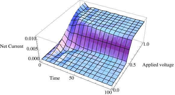
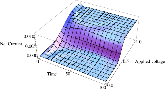
Figure 3: Net current ($I_{L}(t)-I_{R}(t)$) flowing through the system as a function of both time and of the left Fermi level for two different values of coupling strength: $\eta=0.02$ (Fig. 3(a)), and $0.1$ (Fig. 3(b)). Parameters: $\epsilon_{0}=0.5,\epsilon_{FR}=0,\epsilon_{FL}=1,\hbar\omega=0.1,\Gamma=0.01$. Units: all the parameters have same dimension as of $\hbar\omega$.

Figure 4: Net current ($I_{L}(t)-I_{R}(t)$) flowing through the system as a function of time for two different values of coupling strength: $\eta=0.02$ (dotted line), and $0.08$ (solid line). Parameters: $\epsilon_{0}=0.5,\epsilon_{FR}=0,\epsilon_{FL}=1,\hbar\omega=0.1,\Gamma=0.01$. Units: all the parameters have same dimension as of $\hbar\omega$.

Figure 5: Net current ($I_{L}(t)-I_{R}(t)$) flowing through the system as a function of time for two different values of coupling strength: $\eta=0.02$ (dotted line), and $0.08$ (solid line), and $\Gamma=0.1$. All the parameters are same as in fig. 4 and have same dimension as of $\hbar\omega$.

In fig. 3 we have shown the net current ($I_{L}(t)-I_{R}(t)$) flowing through the system as a function of both time and of the left Fermi level for two different values of coupling strength: $\eta=0.02$ to $\eta=0.08$ and for small and large values of $\Gamma$. We observe simple oscillations in the net current flowing through the system for weak coupling strength and weak tunneling. With increasing coupling strength the structure of the oscillations becomes more complicated as shown in fig. 3(b). In order to interpret this complicated structure, we have a two step discussion: firstly, we have plotted the net current as a function of time in fig. 4 with fixed values of the Fermi level, $\epsilon_{\mathrm{F}L}=1$, $\epsilon_{\mathrm{F}R}=0,$ tunneling energy, $\Gamma=0.01$ and for different values of coupling strength: $\eta=0.02$ and $\eta=0.08.$ In this figure, in the limit of weak coupling the oscillations are again simple while for the strong coupling limit, there is a beating pattern in the oscillations. We note that the frequency of the simple oscillations is ($\left|\epsilon_{\mathrm{F}L}-\epsilon_{0}\right|$) and these oscillations are present even in the limit of weak coupling. We conclude that this is a purely electronic process (plasmon oscillations). It is clear from the figure that in the strong coupling case, it contains two beating frequencies, therefore we interpret this as due to a mixture of electronic and mechanical frequencies. Secondly, in fig. 5, we have plotted the net current for fixed values of $\epsilon_{\mathrm{F}L}=1$, $\epsilon_{\mathrm{F}R}=0,$ tunneling energy, $\Gamma=\hbar\omega$ and for different values of coupling strength: $\eta=0.02$ and $\eta=0.08.$ We have found that in the regime ( $\Gamma\geq\hbar\omega$), the effects of the oscillator are not apparent and the period of the nanomechanical oscillator can not be resolved. Why can the period of the oscillator not be resolved by the electrons in this limit? In this regime, electrons spend less time on the dot than the period of the oscillator. Therefore, electrons do not resolve the period of the nanomechanical oscillator. Now we will focus only in the regime of small tunneling $\Gamma<\hbar\omega$, for further discussion in order to analyze the dynamics of the nanomechanical oscillator and the effects of coupling between the electrons and the nanomechanical oscillator.

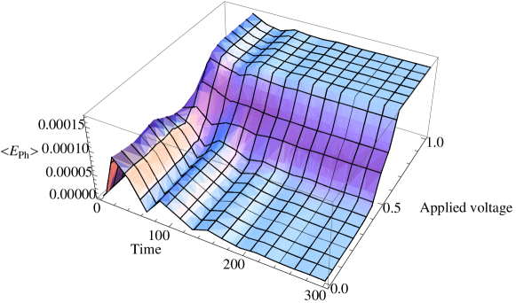
Figure 6: Average energy transferred to the oscillator as a function of time and left Fermi level for fixed values of $\epsilon_{0}=0.5,\epsilon_{FR}=0,\Gamma=0.01$ and for different values of coupling strength: $\eta=0.02$ (Fig. 6(a)), and $0.08$ (Fig. 6(b)). Units: all the parameters have same dimension as of $\hbar\omega$.

Next we have shown the average energy of the nanomechanical oscillator as a function of time and of the left Fermi energy in fig. 6 for fixed values of tunneling $\Gamma=0.01$, $\epsilon_{\mathrm{F}R}=0,$ and for different values of coupling strength $\eta=0.02,$ $\eta=0.08$. We found damped oscillations for short times and constant energy for long times. This constant average energy increases with increasing Fermi level. Why have we found this particular type of structure? We know that the nanomechanical oscillator potential seen by the electrons on the dot is independent of time when the oscillator is in any of its pure eigenstates. Otherwise, when the oscillator is not in a pure state, the potential seen by the electrons is time dependent. In the former case, the electrons are scattered elastically by the time independent potential and in the latter case the scattering process is inelastic because the time dependent potential allow the transfer of energy between the two. We observe that the constant average energy also has steps as a function of the left Fermi level which become more pronounced with increasing coupling strength. Hence, the oscillatory part of the behavior of the mechanical oscillator is damped by coupling with the electrons on the dot but the constant part is not. The damping mechanism in the transient dynamics is due to transfer of energy from the nanomechanical oscillator to the electrons on the dot while when the oscillator is in any of the pure eigenstate then there is no mechanism for the transfer of energy between the two. This same physical phenomenon also applies to the net current flowing through the dot as well. This appear to be a specifically new quantum phenomena in the study of nanomechanical systems.

Figure 7: Average energy transferred to the oscillator as a function of $\frac{\hbar^{\prime}}{\hbar}$ and for fixed values of $\epsilon_{0}=0.5,t=1000,\epsilon_{FR}=0,\epsilon_{FL}=1,\Gamma=1$ and $\eta=0.02$. Units: all the parameters have same dimension as of $\hbar\omega$.

Can we compare this quantum phenomena with the classical mechanical oscillator? Yes, the nanomechanical oscillator has to enter the classical regime in the limit of small $\hbar$. For this, we study the dynamics of the quantum oscillator in the classical limit, in which $\hbar$ in the mechanical oscillator part of the Hamiltonian given in Eq. (1) goes to zero, where $\hbar\omega<\Gamma$ . To see this, we have plotted the average energy as a function of $Y=\frac{\hbar^{\prime}}{\hbar}$ in the nanomechanical part of the system in fig. 7 for fixed values of tunneling $\Gamma=1$, $\epsilon_{\mathrm{F}R}=0,\epsilon_{\mathrm{F}L}=1$ and coupling strength $\eta=0.05$. We found that the average energy of the quantum nanomechanical oscillator scales as $\hbar^{2}$. We set the average energy in the limit $\hbar^{\prime}\rightarrow 0$ to see what happen to the system for long time. It implies that in this limit, the energy transferred to the nanomechanical oscillator is zero for long time. Hence, we conclude that the long time dynamics of the classical mechanical oscillator is always zero.

Figure 8: Fano factor as a function of time for two different values of coupling strength: $\eta=0.02$ (dotted line), and $0.08$ (solid line). Parameters: $\epsilon_{0}=0.5,\epsilon_{FR}=0,\epsilon_{FL}=1,\hbar\omega=0.1,\Gamma=0.01$. Units: all the parameters have same dimension as of $\hbar\omega$.

Finally, in fig. 8, we have shown the Fano factor as a function of time for two different values of $\eta=0.02,\eta=0.08$ and for fixed values of $\Gamma=0.01,\epsilon_{\mathrm{F}R}=0,\epsilon_{\mathrm{F}L}=1$. In the limit of weak coupling, the nanomechanical oscillator shows thermal like behavior and poissonian statistics while in the limit of strong coupling its dynamics is non-thermal which leads to super-poissonian statistics. In this figure, the short time behavior is always thermal, but this is trivial as the nanomechanical oscillator is initially in its ground state.

In conclusion, we have found mixed and pure states in our results which confirm the quantum dynamics of our model with the following justifications: in a classical mechanical oscillator model15 ; 16 ; 17 ; 47 all states give rise to a time dependent potential. Hence, all states of the classical mechanical oscillator are damped. Thus, we confirm the new quantum dynamics of the nanomechanical oscillator that will be helpful for further experiments beyond the classical limit to develop better understanding of NEMS devices.

VII Summary

In this work, we analyzed the time-dependent quantum transport of a resonant tunnel junction coupled to a nanomechanical oscillator by using the nonequilibrium Green’s function approach without treating the electron phonon coupling as a perturbation. We have derived an expression for the full density matrix or the dot population and discuss it in detail for different values of the coupling strength and the tunneling rate. We derive an expression for the current to see the effects of the coupling of the electrons to the oscillator on the dot and the tunneling rate of electrons to resolve the dynamics of the nanomechanical oscillator. This confirms that electrons resolve the dynamics of nanomechanical oscillator in the regime $\tau_{e}>\tau_{\text{Osc}}$ while they do not in the opposite case $\tau_{e}>\tau_{\text{Osc}}.$ Furthermore, we discuss the average energy transferred to oscillator as a function of time. We also discuss the Fano factor as a function of time, which shows thermal behavior and poissonian to non-thermal and super-poissonian behavior. We have found new dynamics of the nanomechanical oscillator: pure and mixed states, which are never present in a classical oscillator. These results suggest further experiments for NEMS to go beyond the classical dynamics.

Appendix A

The particle current $I_{\alpha}$ into the interacting region from the lead is related to the expectation value of the time derivative of the number operator $N_{\alpha}=\sum_{\alpha j}c_{\alpha j}^{\dagger}c_{\alpha j}$, as25 ; 35 ; 36 ; 37

$$I_{\alpha}(t) = -e\langle\frac{d}{dt}x\rangle=\frac{-\mathrm{i}e}{\hbar}\langle[H,x]\rangle$$ (23)

$$I_{\alpha}(t) = \frac{e}{\hbar}\{\operatorname{G}_{0,\alpha}^{<}(t,t)V_{\alpha,0}(t)-V_{0,\alpha}^{\ast}(t)\operatorname{G}_{\alpha,0}^{<}(t,t)\},$$ (24)

where we have the following relations

$$\operatorname{G}_{o,\alpha}^{<}(t,t) = {\displaystyle\int}\mathrm{d}t^{\prime}\left\{\operatorname{G}_{0,0}^{r}(t,t^{\prime})V_{0,\alpha}(t^{\prime})\operatorname{g}_{\alpha,\alpha}^{<}(t^{\prime},t)+\operatorname{G}_{0,0}^{<}(t,t^{\prime})V_{0,\alpha}(t^{\prime})\operatorname{g}_{\alpha,\alpha}^{a}(t^{\prime},t)\right\}$$ (25)

$$\operatorname{G}_{\alpha,0}^{<}(t,t) = {\displaystyle\int}\mathrm{d}t^{\prime}\left\{\operatorname{g}_{\alpha,\alpha}^{r}(t,t^{\prime})V_{\alpha,0}(t^{\prime})\operatorname{G}_{0,0}^{<}(t^{\prime},t)+\operatorname{g}_{\alpha,\alpha}^{<}(t,t^{\prime})V_{\alpha,0}(t^{\prime})\operatorname{G}_{0,0}^{a}(t^{\prime},t)\right\},$$ (26)

where $\operatorname{g}_{\alpha,\alpha}^{r,(a),(<)}(t,t^{\prime})$ refers to the unperturbed states of the leads and given as

$$\operatorname{g}_{\alpha,\alpha}^{r}(t,t^{\prime})=\frac{1}{N}\sum_{j}\operatorname{g}_{\alpha,j}^{r}(t,t^{\prime})=-\mathrm{i}n_{\alpha}\theta(t-t^{\prime})\overset{+\infty}{\underset{-\infty}{{\displaystyle\int}}}\mathrm{d}\varepsilon_{\alpha}\exp[-\mathrm{i}\varepsilon_{\alpha}(t-t^{\prime})],$$

with the fact that $\underset{j}{{\displaystyle\sum}}\mapsto\overset{+\infty}{\underset{-\infty}{{\displaystyle\int}}}Nn_{\alpha}\mathrm{d}\varepsilon_{\alpha}$ with $n_{\alpha}$ being the constant number density of the leads and other uncoupled Green’s function in the leads are

$$\operatorname{g}_{\alpha,\alpha}^{a}(t,t^{\prime}) = \frac{1}{N}\underset{j}{{\displaystyle\sum}}\operatorname{g}_{\alpha,j}^{a}(t,t^{\prime})=+\mathrm{i}n_{\alpha}\theta(t^{\prime}-t)\overset{+\infty}{\underset{-\infty}{{\displaystyle\int}}}\mathrm{d}\varepsilon_{\alpha}\exp[-\mathrm{i}\varepsilon_{\alpha}(t-t^{\prime})],$$

$$\operatorname{g}_{\alpha,\alpha}^{<}(t,t^{\prime}) = \frac{1}{N}\underset{j}{{\displaystyle\sum}}\operatorname{f}_{\alpha}(\varepsilon_{\alpha})g_{\alpha,j}^{<}(t,t^{\prime})=\overset{+\infty}{\underset{-\infty}{{\displaystyle\int}}}\mathrm{d}\varepsilon_{\alpha}\operatorname{f}_{\alpha}(\varepsilon_{\alpha})\mathrm{i}n_{\alpha}\exp[-\mathrm{i}\varepsilon_{\alpha}(t-t^{\prime})],$$

Now using equations (25 & 26) in the equation (24) of current through lead $\alpha$ as

$$I_{\alpha}(t) = \frac{e}{\hbar}{\displaystyle\int}\mathrm{d}t^{\prime}\operatorname{Tr}\left\{\left(\operatorname{G}_{0,0}^{r}(t,t^{\prime})V_{0,\alpha}(t^{\prime})\operatorname{g}_{\alpha,\alpha}^{<}(t^{\prime},t)+\operatorname{G}_{0,0}^{<}(t,t^{\prime})V_{0,\alpha}(t^{\prime})\operatorname{g}_{\alpha,\alpha}^{a}(t^{\prime},t)\right)V_{\alpha,0}(t)\right.$$ (27)

$$-\left.V_{0,\alpha}^{\ast}(t)\left(\operatorname{g}_{\alpha,\alpha}^{r}(t,t^{\prime})V_{\alpha,0}(t^{\prime})\operatorname{G}_{0,0}^{<}(t^{\prime},t)+\operatorname{g}_{\alpha,\alpha}^{<}(t,t^{\prime})V_{\alpha,0}(t^{\prime})\operatorname{G}_{0,0}^{a}(t^{\prime},t)\right)\right\},$$

Using the fact that $\Sigma_{0,0,\alpha}^{r,(a),(<)}(t^{\prime},t)=V_{0,\alpha}^{\ast}(t^{\prime})\operatorname{g}_{\alpha,\alpha}^{r,(a),(<)}(t^{\prime},t)V_{\alpha,0}(t)$, we can simplify the above equation as

$$I_{\alpha}(t) = \frac{e}{\hbar}{\displaystyle\int}\mathrm{d}t^{\prime}\operatorname{Tr}\left\{\operatorname{G}_{0,0}^{r}(t,t^{\prime})\Sigma_{0,0,\alpha}^{<}(t^{\prime},t)+\operatorname{G}_{0,0}^{<}(t,t^{\prime})\Sigma_{0,0,\alpha}^{a}(t^{\prime},t)\right.$$ (28)

$$-\left.\Sigma_{0,0,\alpha}^{r}(t,t^{\prime})G_{0,0}^{<}(t^{\prime},t)-\Sigma_{0,0,\alpha}^{<}(t,t^{\prime})G_{0,0}^{a}(t^{\prime},t)]\right\},$$

where $\Sigma_{0,0,\alpha}^{r,(a),(<)}(t,t^{\prime})$ are non-zero only when both the times ($t,t^{\prime}$) are positive $t,t^{\prime}>0$. Although $\operatorname{g}^{r,(a)}(t,t^{\prime})$ is non-zero for $t<0$, it is never required due to the way it combines with $\Sigma_{0,0,\alpha}^{r,(a),(<)}(t,t^{\prime})$. Here we note that we require $\operatorname{g}^{r,(a)}(t,t^{\prime})$ from Eq. (14 & 15) for positive times only ($t>0)$. The first integral on right hand side of Eq. (28) may be solved by using Eq. (13, 14 & 17) as

$$\operatorname{Tr}{\displaystyle\int_{0}^{t}}\mathrm{d}t^{\prime}\operatorname{G}_{0,0}^{r}(t,t^{\prime})\Sigma_{0,0,\alpha}^{<}(t^{\prime},t)$$ (29)

$$= \frac{-\Gamma}{2\pi}\sum_{m}{\displaystyle\int\limits_{-\infty}^{\epsilon_{\mathrm{F}\alpha}}}\mathrm{d}\varepsilon_{\alpha}{\displaystyle\int_{0}^{t}}\mathrm{d}t^{\prime}\Phi_{0,m}\Phi_{0,m}^{\ast}\exp[-\mathrm{i}(\varepsilon_{m}-\mathrm{i}\Gamma)(t-t^{\prime})]\exp[-\mathrm{i}\varepsilon_{\alpha}(t^{\prime}-t)]$$

$$= \frac{\mathrm{i}\Gamma}{2\pi}\sum_{m}\Phi_{0,m}\Phi_{0,m}^{\ast}{\displaystyle\int\limits_{-\infty}^{\epsilon_{\mathrm{F}\alpha}}}\mathrm{d}\varepsilon_{\alpha}\left\{\frac{1-\exp[\mathrm{i}(\varepsilon_{\alpha}-\varepsilon_{m}+\mathrm{i}\Gamma)t]}{\varepsilon_{\alpha}-\varepsilon_{m}+\mathrm{i}\Gamma}\right\}$$

$$= \frac{\mathrm{i}\Gamma}{2\pi}\sum_{m}\Phi_{0,m}\Phi_{0,m}^{\ast}\left\{\ln(\epsilon_{\mathrm{F}\alpha}-\varepsilon_{m}+\mathrm{i}\Gamma)-\operatorname{Ei}[\mathrm{i}(\epsilon_{\mathrm{F}\alpha}-\varepsilon_{m}+\mathrm{i}\Gamma)t]\right\},$$

where the final result is obtained using standard integrals45 . We note once again that special care is required in evaluating the $\ln(x)$ and $\operatorname{Ei}(x)$ to choose the correct Riemann sheets in order to make sure that these functions are consistent with the initial conditions and are continuous functions of time and chemical potential. This statement will also apply to all further discussions.

The second & third integral on right hand side of Eq. (28) are written as

$$\operatorname{Tr}{\displaystyle\int_{0}^{t}}\mathrm{d}t^{\prime}\left\{\operatorname{G}_{0,0}^{<}(t,t^{\prime})\Sigma_{0,0,\alpha}^{a}(t^{\prime},t)-\Sigma_{0,0,\alpha}^{r}(t,t^{\prime})\operatorname{G}_{0,0}^{<}(t^{\prime},t)\right\}=\mathrm{i}\Gamma\operatorname{Tr}\operatorname{G}_{0,0}^{<}(t,t).$$

This integral can be solved in the same way as for the dot population. The final result is written as45

$$\mathrm{i}\Gamma\operatorname{Tr}\operatorname{G}_{0,0}^{<}(t,t) = \frac{\Gamma}{2\pi}\sum_{\alpha,m}\Phi_{0,m}\Phi_{0,m}^{\ast}\biggl{\{}-\left(1+\exp[-2\Gamma t]\right)\left(\tan^{-1}\left[\frac{\epsilon_{\mathrm{F}\alpha}-\varepsilon_{m}}{\Gamma}\right]+\frac{\pi}{2}\right)$$ (30)

$$+\mathchoice{{\textstyle{\frac{1}{2}}}}{{\textstyle{\frac{1}{2}}}}{{\scriptstyle{1/2}}}{{\scriptscriptstyle{1/2}}}\mathrm{i}\exp[-2\Gamma t]\left(-\operatorname{Ei}[+\mathrm{i}(\epsilon_{\mathrm{F}\alpha}-\varepsilon_{m}-\mathrm{i}\Gamma)t]+\operatorname{Ei}[-\mathrm{i}(\epsilon_{\mathrm{F}\alpha}-\varepsilon_{m}+\mathrm{i}\Gamma)t]\right)$$

$$+\mathchoice{{\textstyle{\frac{1}{2}}}}{{\textstyle{\frac{1}{2}}}}{{\scriptstyle{1/2}}}{{\scriptscriptstyle{1/2}}}\mathrm{i}\left(\operatorname{Ei}[+\mathrm{i}(\epsilon_{\mathrm{F}\alpha}-\varepsilon_{m}+\mathrm{i}\Gamma)t]-\operatorname{Ei}[-\mathrm{i}(\epsilon_{\mathrm{F}\alpha}-\varepsilon_{m}-\mathrm{i}\Gamma)t]\right)\biggr{\}},$$

and the fourth integral on right hand side of equation (28) can be solved by using Eq. (13, 15, & 17) as

$$-\operatorname{Tr}{\displaystyle\int_{0}^{t}}\mathrm{d}t^{\prime}\Sigma_{0,0,\alpha}^{<}(t,t^{\prime})\operatorname{G}_{0,0}^{a}(t^{\prime},t)$$ (31)

$$= \frac{\Gamma}{2\pi}\sum_{m}{\displaystyle\int\limits_{-\infty}^{\epsilon_{\mathrm{F}\alpha}}}d\varepsilon_{\alpha}{\displaystyle\int_{0}^{t}}\mathrm{d}t^{\prime}\Phi_{0,m}\Phi_{0,m}^{\ast}\exp[-\mathrm{i}(\varepsilon_{m}+\mathrm{i}\Gamma)(t^{\prime}-t)]\exp[-\mathrm{i}\varepsilon_{\alpha}(t-t^{\prime})]$$

$$= \frac{-\mathrm{i}\Gamma}{2\pi}\sum_{m}\Phi_{0,m}\Phi_{0,m}^{\ast}{\displaystyle\int\limits_{-\infty}^{\epsilon_{\mathrm{F}\alpha}}}\mathrm{d}\varepsilon_{\alpha}\left\{\frac{1-\exp[-\mathrm{i}(\varepsilon_{\alpha}-\varepsilon_{m}-\mathrm{i}\Gamma)t}{\varepsilon_{\alpha}-\varepsilon_{m}-\mathrm{i}\Gamma}\right\}$$

$$= \frac{-\mathrm{i}\Gamma}{2\pi}\sum_{m}\Phi_{0,m}\Phi_{0,m}^{\ast}\left\{\ln(\epsilon_{\mathrm{F}\alpha}-\varepsilon_{m}-\mathrm{i}\Gamma)-\operatorname{Ei}[-\mathrm{i}(\epsilon_{\mathrm{F}\alpha}-\varepsilon_{m}-\mathrm{i}\Gamma)t]\right\}$$

Using equations (29, 30 & 31) in Eq. (28), the final expression for the current is written as

$$I_{\alpha}(t)=\frac{e\Gamma}{2\pi\hbar}\sum_{m}\Phi_{0,m}\Phi_{0,m}^{\ast}\{I^{1\alpha}_{m}+I^{2L}_{m}+I^{2R}_{m}\},$$ (32)

where components of current are written as

$$I^{1\alpha}_{m} = 2\left(\tan^{-1}\left[\frac{\epsilon_{\mathrm{F}\alpha}-\varepsilon_{m}}{\Gamma}\right]+\frac{\pi}{2}\right)$$

$$-\mathrm{i}\left\{\operatorname{Ei}[+\mathrm{i}(\epsilon_{\mathrm{F}\alpha}-\varepsilon_{m}+\mathrm{i}\Gamma)t]-\operatorname{Ei}[-\mathrm{i}(\epsilon_{\mathrm{F}\alpha}-\varepsilon_{m}-\mathrm{i}\Gamma)t]\right\}],$$

$$I^{2\alpha}_{m} = -\left(1+\exp[-2\Gamma t]\right)\left\{\tan^{-1}\left[\frac{\epsilon_{\mathrm{F}\alpha}-\varepsilon_{m}}{\Gamma}\right]+\frac{\pi}{2}\right\}$$

$$-\mathchoice{{\textstyle{\frac{1}{2}}}}{{\textstyle{\frac{1}{2}}}}{{\scriptstyle{1/2}}}{{\scriptscriptstyle{1/2}}}\mathrm{i}\exp[-2\Gamma t]\left\{\operatorname{Ei}[+\mathrm{i}(\epsilon_{\mathrm{F}\alpha}-\varepsilon_{m}-\mathrm{i}\Gamma)t]-\operatorname{Ei}[-\mathrm{i}(\epsilon_{\mathrm{F}\alpha}-\varepsilon_{m}+\mathrm{i}\Gamma)t]\right\}$$

$$+\mathchoice{{\textstyle{\frac{1}{2}}}}{{\textstyle{\frac{1}{2}}}}{{\scriptstyle{1/2}}}{{\scriptscriptstyle{1/2}}}\mathrm{i}\left\{\operatorname{Ei}[+\mathrm{i}(\epsilon_{\mathrm{F}\alpha}-\varepsilon_{m}+\mathrm{i}\Gamma)t]-\operatorname{Ei}[-\mathrm{i}(\epsilon_{\mathrm{F}\alpha}-\varepsilon_{m}-\mathrm{i}\Gamma)t]\right\},$$

where in calculating the left current we need $I^{1L}_{m}$ together with both $I^{2L}_{m}$ and $I^{2R}_{m}$ whereas for the right current $I^{1L}_{m}$ is replaced by $I^{1R}_{m}$.

Acknowledgement 1

M.Tahir would like to acknowledge the support of the Pakistan Higher Education Commission (HEC).

References

- (1) A. Schliesser, et. al., Nature Physics 5, 509 (2009);, K. L. Ekinci and M. L. Roukes, Review of Scientific Instruments 76, 061101 (2005).; K. L. Ekinci, Small 2005,1, No. 8-9, 786-797.; M. L. Roukes, Technical Digest of the 2000 Solid State Sensor and Actuator Workshop; “Nanoelectromechanical Systems”.; H. G. Craighead, Science 290, 1532 (2000).; P. Kim and C. M. Lieber, Science 126, 2148 (1999).
- (2) S. D. Bennett, and A.A. Clerk, Phys. Rev. B 78, 165328 (2008).; S. Akita, Y. Nakayama, S. Mizooka, Y. Takano, T. Okawa, Y. Miyatake, S. Yamanaka, M. Tsuji, and T. Nosaka, Appl. Phys. Lett. 79, 1691 (2001).; A. M. Fennimore, T. D. Yuzvlnsky, W. Q. Han, M. S. Fuhrer, J. Cummings, and A. Zettl, Nature 424, 408 (2003).
- (3) J. Kinaret, T. Nord, and S. Viefers, Appl. Phys. Lett. 82, 1287 (2003).; C.-H. Ke and H. D. Espinosa, Appl. Phys. Lett. 85, 681 (2004).; V. Sazonova, Y. Yaish, H. Üstünel, D. Roundy, T. Arias, and P. McEuen, Nature 431, 284 (2004).
- (4) M. P. Blencowe, Phys. Rep. 395, 159 (2004).; A. N. Cleland, Foundations of Nanomechanics, 2003 (Berlin: Springer).
- (5) H. Park et al., Nature (London) 407, 57 (2000).J. Koch and F. von Oppen, Phys. Rev. Lett. 94, 206804 (2005).; J. Koch, M. E. Raikh, and F. von Oppen, ibid. 95, 056801 (2005).; J. Koch, F. von Oppen, and A. V. Andreev, Phys. Rev. B 74, 205438 (2006).
- (6) M. A. Reed, C. Zhou, C. J. Muller, T. P. Burgin, and J. M. Tour, Science 278, 252 (1997).; R. H. M. Smit, Y. Noat, C. Untiedt, N. D. Lang, M. C. van Hemert, and J. M. van Ruitenbeek, ibid. 419, 906 (2002).
- (7) L. H. Yu, Z. K. Keane, J. W. Ciszek, L. Cheng, M. P. Stewart, J. M. Tour, and D. Natelson, Phys. Rev. Lett. 93, 266802 (2004).; L. H. Yu and D. Natelson, Nano Lett. 4, 79 (2004).; M. Elbing, R. Ochs, M. Koentopp, M. Fischer, C. von Hänisch, F. Weigend, F. Evers, H. B. Weber, and M. Mayor, Proc. Natl. Acad. Sci. U.S.A. 102, 8815 (2005).; M. Poot, E. Osorio, K. O’Neill, J. M. Thijssen, D. Vanmaekelbergh, C. A. van Walree, L. W. Jenneskens, and H. S. J. van der Zant, Nano Lett. 6, 1031 (2006).
- (8) E. A. Osorio, K. O’Neill, N. Stuhr-Hansen, O. F. Nielsen, T. Bjørnholm, and H. S. J. van der Zant, Adv. Mater. (Weinheim, Ger.) 19, 281 (2007).; E. Lörtscher, H. B. Weber, and H. Riel, Phys. Rev. Lett. 98, 176807 (2007).
- (9) R. G. Knobel and A. N. Cleland, Nature 424, 291 (2003).; M. Poggio et al., Nature 4, 635 (2008).
- (10) A. Naik et al., Nature (London) 443, 193 (2006).
- (11) B. J. LeRoy et al., Nature 432, 371 (2004).
- (12) S. J. Bunch, et al., Science 315, 490 (2007).
- (13) L. Y. Gorelik, et al. , Phys. Rev. Lett. 80, 4526 (1998).; T. Novotný, A. Donarini, and A.-P. Jauho, ibid. 90, 256801 (2003).
- (14) J. Koch and F. von Oppen, Phys. Rev. Lett. 94, 206804 (2005).; J. Koch, F. von Oppen, and A. V. Andreev, Phys. Rev. B 74, 205438 (2006).
- (15) A. Yu. Smirnov, L. G. Mourokh, and N. J. M. Horing, Phys. Rev. B 67, 115312 (2003).
- (16) A. D. Armour, M. P. Blencowe, and Y. Zhang, Phys. Rev. B 69, 125313 (2004).
- (17) C. B. Doiron, W. Belzig, and C. Bruder, Phys. Rev. B 74, 205336 (2006).
- (18) D. Mozyrsky, and I. Martin, Phys. Rev. Lett. 89, 018301 (2002).; D. Mozyrsky, I. Martin, and M. B. Hastings, Phys. Rev. Lett. 92, 018303 (2004).
- (19) M. D. La Haye et al., Science 304, 74 (2004).; K. C. Schwab and M. L. Roukes, Phys. Today 58 (7), 36 (2005).
- (20) F. Pistolesi, Y.M. Blanter and I. Martin, Phys. Rev. B 78, 085127 (2008) and references therein.; A. Mitra, I. Aleiner and A. J. Millis, Phys. Rev. B 69, 245302 (2004).
- (21) J. Repp, G. Meyer, S. M. Stojković, A. Gourdon, and C. Joachim, Phys. Rev. Lett. 94, 026803 (2005).; J. Repp, G. Meyer, S. Paavilainen, F. E. Olsson, and M. Persson, Phys. Rev. Lett. 95, 225503 (2005).
- (22) S. W. Wu, G. V. Nazin, X. Chen, X. H. Qiu, and W. Ho, Phys. Rev. Lett. 93, 236802 (2004).; X. H. Qiu, G. V. Nazin, and W. Ho, Phys. Rev. Lett. 92, 206102 (2004).
- (23) A. Shimizu and M. Ueda, Phys. Rev. Lett. 69, 1403 (1992) ; O. L. Bo and Yu. Galperin, Phys. Rev. B 55, 1696 (1997) ; B. Dong, H. L. Cui, X. L. Lei, and N. J. M. Horing, Phys. Rev. B 71, 045331 (2005) ; Y.-C. Chen and M. Di Ventra, Phys. Rev. Lett. 95,166802 (2005).
- (24) L. V. Keldysh, Zh. Eksp. Teor. Fiz. 47, 1515 (1965).
- (25) H. Huagand A. P. Jauho, Quantum Kinetics in Transport and Optics of Semiconductors, Springer Solid-State Sciences Vol. 123 (Springer, New York, 1996).
- (26) S. Datta, J. Phys.: Condens. Matter 2, 8023 (1990); R. Lake and S. Datta, Phys. Rev. B 45, 6670 (1992); 46, 4757 (1992).
- (27) N. Nishiguchi, Phys. Rev. Lett. 89, 066802 (2002); A. A. Clerk and S. M. Girvin, Phys. Rev. B 70, 121303(R) (2004); T. Novotný, A. Donarini, C. Flindt, and A.-P.Jauho, Phys. Rev. Lett. 92, 248302 (2004).
- (28) A. D. Armour and A. MacKinnon, Phys. Rev. B 66, 035333 (2002); C. Flindt, T. Novotny, and A.-P. Jauho, Phys. Rev. B 70, 205334 (2004); J. Wabnig, D. V. Khomitsky, J. Rammer, and A. L. Shelankov, Phys. Rev. B 72,165347 (2005).
- (29) M. Galperin, M. A. Ratner, and A. Nitzan, J. Chem. Phys. 121, 11965 (2004).; J. Phys.: Condens. Matter 19, 103201 (2007).; R. Hartle, C. Benesch, and M. Thoss, Phys. Rev. B 77, 205314 (2008).
- (30) J. Aghassi, A. Thielmann, M. H. Hettler, and G. Schön, Appl. Phys. Lett. 89, 052101 (2006); M. Kindermann and P. W. Brouwer, Phys. Rev. B 74, 125309 (2006).
- (31) D. B. Gutman and Y. Gefen, Phys. Rev. B 64, 205317 (2001).
- (32) E. B. Sonin, Phys. Rev. B 70, 140506(R) (2004); E. B. Sonin, J. Low Temp. Phys. 146, 161 (2007).
- (33) S. Dallakyan and S. Mazumdar, Appl. Phys. Lett. 82, 2488 (2003); K. Walczak, Phys. Status Solidi B 241, 2555 (2004); Y.-C. Chen and M. Di Ventra, Phys. Rev. B 67, 153304 (2003); J. Lagerqvist, Y.-C. Chen, and M. Di Ventra, Nanotechnology 15, S459 (2004).
- (34) V. Aji, J. E. Moore, and C. M. Varma, arXiv:cond-mat/0302222 (unpublished).; Dmitry A. Ryndyk and Gianaurelio Cuniberti, Phys. Rev. B 76, 155430 (2007).; J.-X. Zhu and A. V. Balatsky, Phys. Rev. B 67, 165326 (2003).; M. Tahir and A. MacKinnon, Phys. Rev. B 77, 224305 (2008).
- (35) Ned S. Wingreen, Karsten W. Jacobsen, and John W. Wilkins, Phys. Rev. B 40, 11834 (1989).; A. P. Jauho, N. S. Wingreen, and Y. Meir, Phys. Rev. B 50, 5528 (1994).
- (36) V. Moldoveanu, V. Gudmundsson and A. Manolescu, Phys. Rev. B 76, 085330 (2007).; J. Maciejko, J. Wang and H. Guo, Phys. Rev. B 74, 085324 (2006).; Y. Wei and J. Wang, Phys. Rev. B 79, 195315 (2009).; P. Myöhänen, A. Stan, G. Stefanucci and R. van Leeuwen, Phys. Rev. B 80, 115107 (2009).; A. R. Hernández, F. A. Pinheiro, C. H. Lewenkopf, and E.R. Mucciolo, Phys. Rev. B 80, 115311 (2009).
- (37) T. L. Schmidt, P. Werner, L. Mühlbacher, and A. Komnik, Phys. Rev. B 78, 235110 (2008).; J. Maciejko, J. Wang, and H. Guo, Phys. Rev. B 74, 085324 (2006).
- (38) P. Nordlander, M. Pustilnik, Y. Meir, N. S. Wingreen, and D. C. Langreth, Phys. Rev. Lett. 83, 808 (1999). M. Plihal, D. C. Langreth, and P. Nordlander, Phys. Rev. B 71, 165321 (2005).
- (39) A. Goker, B. A. Friedman, and P. Nordlander, J. Phys.: Condens. Matter 19, 376206 (2007). A. Komnik, arXiv:0903.3344v1(unpublished).
- (40) R.-P. Riwar and T. L. Schmidt, Phys. Rev. B 80, 125109 (2009), and refernces therein.
- (41) H. Hübener and T. Brandes, Phys. Rev. B 80, 155437 (2009).; S. Ramakrishnan, Y. Gulak and H. Benaroya, Phys. Rev. B 78, 174304 (2008).; G. Kiesslich, E. Schöll, T. Brandes, F. Hohls, and R. J. Haug, Phys. Rev. Lett. 99, 206602 (2007).; H. Hübener and T. Brandes, Phys. Rev. Lett. 99, 247206 (2007).
- (42) Michael Galperin, Abraham Nitzan, and Mark A. Ratner, Phys. Rev. B 74, 075326 (2006).; V. Nam Do, P. Dollfus, and V. Lien Nguyen, Appl. Phys. Lett. 91, 022104 (2007).
- (43) Michael Galperin, Abraham Nitzan, and Mark A. Ratner, Phys. Rev. B 73, 045314 (2006).; Nano Lett. 4, 1605 (2004).
- (44) I. S. Gradshteyn and I. M. Ryzhik, Tables of Integrals, Series and Products Academic, New York, (1980), P. 837.
- (45) I. S. Gradshteyn and I. M. Ryzhik, Tables of Integrals, Series and Products Academic, New York, (1980), P. 311.
- (46) T. Brandes and N. Lambert, Phys. Rev. B 67, 125323 (2003),; D. A. Rodrigues, J. Imbers, and A. D. Armour, Phys. Rev. Lett. 98, 067204 (2007).
- (47) F. Pistolesi, and S. Labarthe, Phys. Rev. B 76, 165317 (2007).