Vorticity of IGM Velocity Field on Large Scales

Abstract

We investigate the vorticity of the IGM velocity field on large scales with cosmological hydrodynamic simulation of the concordance model of $\Lambda$CDM. We show that the vorticity field is significantly increasing with time as it can effectively be generated by shocks and complex structures in the IGM. Therefore, the vorticity field is an effective tool to reveal the nonlinear behavior of the IGM, especially the formation and evolution of turbulence in the IGM. We find that the vorticity field does not follow the filaments and sheets structures of underlying dark matter density field and shows highly non-Gaussian and intermittent features. The power spectrum of the vorticity field is then used to measure the development of turbulence in Fourier space. We show that the relation between the power spectra of vorticity and velocity fields is perfectly in agreement with the prediction of a fully developed homogeneous and isotropic turbulence in the scale range from $0.2$ to about $3h^{-1}$ Mpc at $z\sim 0$. This indicates that cosmic baryonic field is in the state of fully developed turbulence on scales less than about 3 $h^{-1}$ Mpc. The random field of the turbulent fluid yields turbulent pressure to prevent the gravitational collapsing of the IGM. The vorticity and turbulent pressure are strong inside and even outside of high density regions. In IGM regions with 10 times mean overdensity, the turbulent pressure can be on an average equivalent to the thermal pressure of the baryonic gas with a temperature of $1.0\times 10^{5}$ K. Thus, the fully developed turbulence would prevent the baryons in the IGM from falling into the gravitational well of dark matter halos. Moreover, turbulent pressure essentially is dynamical and non-thermal, which makes it different from pre-heating mechanism as it does not affect the thermal state and ionizing process of hydrogen in the IGM.

1 Introduction

Gravity is curl-free in nature, therefore it is unable to trigger vorticity within the velocity field of a cosmic flow. On the linear order of cosmological perturbation theory, the vorticity will inevitably decay due to the expansion of the universe. The linear velocity fields of the cosmic flow should be irrotational. In the nonlinear regime of clustering, vorticity can be generated in the collisionless dark matter field when multi-streaming occurs at shell crossing (Binney, 1974, Pichon & Bernardeau, 1999). However, there is no way to directly map the vorticity of the dark matter field to the baryon field, most of which is the intergalactic medium (IGM).

In the context of fluid dynamics, vorticity can be generated if the gradient of the mass density and the pressure gradient of cosmic flow are not aligned (Landau & Lifshitz 1987). Namely, vorticity results from the complex structures of fluid flow like curved shocks. Recently, it has been revealed that in the nonlinear regime, the cosmic baryon fluid at low redshift does contain such complex structures (e.g. He et al 2004). Therefore, one expects that vorticity would be present and evolve extensively in the cosmic baryonic field. The vorticity of the intracluster medium (ICM) has been studied in topics related to possible mechanism of generating magnetic field of galaxies or clusters (Davis & Widrow 2000; Ryu, et al 2008). Although these works show that the vorticity can form in the ICM, the formation and evolution of vorticity in the IGM is still unknown.

In addition, no studies have been done on the relation between vorticity and turbulence in a cosmic baryon fluid. Actually, vortices generally are considered a fundamental ingredient of turbulence and the fluctuations of the vorticity field is an important indicator to describe the turbulence of fluid (e.g. Batchelor, 1959, Schmidt 2007). On the other hand, the study of the turbulence of cosmic fluid on large scales has seen a lot of progress in recent years. The fluctuations of the velocity field of the baryon fluid beyond the Jeans length is shown to be extremely well described by the She-Leveque (SL) scaling (He, et al 2006), which is the generalized scaling of the classical Kolmogorov’s 5/3-law of fully developed turbulence (She & Leveque 1994). The non-Gaussian features of the density field in baryon flows are found to be in good agreement with the log-Poisson cascade (Liu & Fang 2008), which characterizes statistically the hierarchical structure in fully developed turbulence (Dubrulle 1994; She & Waymire 1995; Benzi et al. 1996). Observationally, the intermittence of Ly$\alpha$ transmitted flux of QSO absorption spectrum can also be well explained in terms of log-Poisson hierarchy cascade(Lu et al. 2009). These results suggest that the dynamical behavior of the IGM is similar to a fully developed turbulence in inertial ranges. Therefore, it would be worthwhile to investigate the vorticity fields of the turbulent cosmic fluid.

An important problem related to the vorticity fields of a turbulent fluid is the impact of the turbulent pressure on the clustering of cosmic fluid. It is well known that the random velocity field of a turbulent fluid will play a similar role as thermal pressure and prevent the gravitational collapse in such a fluid (Chandrasekhar, 1951; Bonazzola et al. 1992). In the ICM, this effect has been studied with hydrodynamic simulations (Dolag et al 2005; Iapichino & Niemeyer 2008; Cassano 2009, and reference therein). However, in these works the turbulent pressure is directly identified with the RMS baryon velocity. This identification may be reasonable for the ICM; however, it would be a poor relation on scales larger than clusters, as the RMS baryon velocity cannot separate the velocity fluctuations due to bulk motion from that of turbulence. Obviously, the bulk motion is not going to prevent gravitational collapsing. Since the dynamical equation of vorticity is free from gravity, the vorticity field provides an effective method to pick up the velocity fluctuations within a turbulent flow. The power spectrum of the vorticity field yields a measurement on the scale of velocity fluctuations where turbulence is fully developed. Using this method, we can estimate the turbulent pressure in the IGM and hence study its effect on gravitational clustering.

We will investigate these problems with cosmological hydrodynamic simulation samples of the concordance model of $\Lambda$CDM. In §2, we present the equations governing the dynamics of vorticity and rate of strain field. §3 gives a brief description of the cosmological hydrodynamic simulation of the $\Lambda$CDM model. In §4 we discuss the statistical properties of vorticity on large scales. The nonthermal pressure of turbulent fluid and its effects on clustering of the IGM are addressed in §5. We summarize the basic results of the paper and give concluding remarks in §6. Mathematical equations are given in the Appendix.

2 Theoretical Background

2.1 Dynamical Equation of Vorticity

The dynamics of a fluid is conventionally governed by a set of equations for velocity and density fields $v_{i}(t,{\bf r})$, $\rho(t,{\bf r})$ (Appendix §A.1). An alternative way is to replace the velocity field by their spatial derivatives $\partial_{i}v_{j}$. The velocity derivative tensor $\partial_{i}v_{j}$ can be decomposed into a symmetric component $S_{ij}=(1/2)(\partial_{i}v_{j}+\partial_{j}v_{i})$ and an antisymmetric component $(1/2)(\partial_{i}v_{j}-\partial_{j}v_{i})$(Landau & Lifshitz 1987). The former is the rate of strain and the latter is the vorticity vector $\omega_{i}=\epsilon_{ijk}\partial_{j}v_{k}$, or $\vec{\omega}=\nabla\times{\bf v}$, where $\epsilon_{ijk}$ is the Levi-Civita antisymmetric symbol. For a cosmic baryon fluid (IGM), the dynamical equation of vorticity $\vec{\omega}$ can be derived from the Euler equation as (Appendix §A.1 and §A.2)

$$\frac{D\vec{\omega}}{Dt}\equiv\partial_{t}{\vec{\omega}}+\frac{1}{a}{\bf v}\cdot{\nabla}\vec{\omega}=\frac{1}{a}({\bf S}\cdot{\vec{\omega}}-d{\vec{\omega}}+\frac{1}{\rho^{2}}\nabla\rho\times\nabla p-\dot{a}\vec{\omega}),$$ (1)

where $p$ is the pressure of the IGM, $a(t)$ is the cosmic factor, $d=\partial_{i}v_{i}$ is the divergence of the velocity field, and the vector $[{\bf S}\cdot{\vec{\omega}}]_{i}=S_{ij}\omega_{j}$. Defining a scalar field as $\omega\equiv|{\vec{\omega}}|$, the dynamical equation of $\omega$ is then

$$\frac{D\omega}{Dt}\equiv\partial_{t}{\omega}+\frac{1}{a}{\bf v}\cdot{\nabla}\omega=\frac{1}{a}\left[\alpha\omega-d\omega+\frac{1}{\rho^{2}}\vec{\xi}\cdot(\nabla\rho\times\nabla p)-\dot{a}\omega\right],$$ (2)

where $\vec{\xi}={\vec{\omega}}/\omega$, and $\alpha={\vec{\xi}}\cdot({\vec{\xi}}\cdot\nabla){\bf v}$.

An essential feature of both eqs.(1) and (2) is that they are free from the gravity of mass fields, therefore, the gravitational field of both dark matter and the IGM cannot be a source of the vorticity. Obviously, in the linear regime, only the last term of eqs.(1) and (2) survives. This term is from the cosmic expansion, and makes the vorticity decaying as $a^{-1}$. Thus, the vorticity of the IGM is reasonably negligible in the linear regime.

Equations (1) and (2) show that if the initial vorticity is zero, the vorticity will stay at zero in the nonlinear regime, provided that the term $(1/\rho^{2})\nabla\rho\times\nabla p$ is zero. This term, called baroclinity, characterizes the degree to which the gradient of pressure, $\nabla p$, is not parallel to the gradient of density, $\nabla\rho$.

If the pressure of a baryon gas is a single-variable function of density, e.g. there exists a determined relation for the equation of state $p=p(\rho)$, the vector $\nabla p$ would be parallel to $\nabla\rho$, and then $(1/\rho^{2})\nabla\rho\times\nabla p=0$. Therefore, vorticity cannot be generated even in the nonlinear regime until the single-variable function or determined relation for $p=p(\rho)$ is violated. Physically, once multi-streaming and turbulent flows have developed, complex structures, like curved shocks, will lead to a deviation of the direction of $\nabla p$ from that of $\nabla\rho$. In this case, the $\rho-p$ relation cannot be simply given by an single-variable function equation as $p=p(\rho)$ (He et al 2004) and the baroclinity will no longer be zero.

The term ${\bf S}\cdot{\vec{\omega}}$ on the right hand side of eq.(1) accounts for stretch of vortices drived by strain. The vorticity will be either amplified or attenuated by this term. Actually, this point can be easily seen with eq.(2). If the coefficient $\alpha$ is larger than zero, i.e. $\vec{\xi}$ is in the direction of the eigenvector of tensor $\partial_{j}v_{i}$ with positive eigenvalue, the vorticity will grow at the rate of $\alpha\omega$. Otherwise it would be attenuated. The term $-d\omega$ stands for expansion or contraction of vortices caused by the compressibility of baryon. Since divergence $d=\partial_{j}v_{j}$ is generally negative in regions of clustering, the term $-d\omega$ will lead to an amplification of vorticity in overdense regions.

2.2 Vorticity Effect on IGM Clustering

The effect of vorticity on the IGM clustering can be seen from the dynamic equation of divergence d, which is an indicator of clustering. The equation reads (Appendix §A.3)

$$\frac{Dd}{Dt} \equiv \partial_{t}d+\frac{1}{a}{\bf v}\cdot{\bf\nabla}d$$

$$= \frac{1}{a}\left[\frac{1}{2}\omega^{2}-S_{ij}S_{ij}-\frac{1}{\rho}\nabla^{2}p+\frac{1}{\rho^{2}}(\nabla\rho)\cdot(\nabla p)-\frac{4\pi G}{a}(\rho_{tot}-\rho_{0})-\dot{a}d\right],$$

where $\rho_{tot}$ is the total mass density including both CDM and baryon and $\rho_{0}$ is its mean value. A negative $d$ corresponds to a convergent flow (clustering), while a positive $d$ means a divergent flow. As in the equation (2) for vorticity, there is a term $-\dot{a}d$ coming from the cosmic expansion that leads to dilution of $d$. However, different from eqs.(1) and (2), the gravity effect $-4\pi G(\rho_{tot}-\rho_{0})/a$, $\rho_{0}$ acts as a source term in the divergence equation. This term leads to clustering in regions with $\rho_{tot}>\rho_{0}$, and anti-clustering for $\rho_{tot}<\rho_{0}$.

The term $(\nabla\rho)\cdot(\nabla p)/\rho^{2}$ will be nonzero even when the IGM is barotropic, or the density-pressure relation is a power law $p\propto\rho^{\gamma}$ and $\gamma>0$. The ratio of this term to the gravity is roughly $\sim(t_{infall}/t_{sound})^{2}$, where $t_{infall}\sim(G\rho)^{-1/2}$, and $t_{sound}\sim l/c_{s}$ with the typical scale of density variation $l\sim(\nabla\rho/\rho)^{-1}$ and the speed of sound $c_{s}\sim(\nabla p/\nabla\rho)^{1/2}$ . The value of this ratio defines roughly the Jeans criterion for gravitational instability. In addition, the pressure term $-\nabla^{2}p$ is compatible with $(\nabla\rho)\cdot(\nabla p)/\rho^{2}$ and is likely to be positive in overdense clustering regions. Hence, these two terms are from thermal pressure to resist upon gravitational collapse.

Finally, we examine the effect of the first two terms, the strain $S_{ij}S_{ij}$ and the vorticity $\frac{1}{2}\omega^{2}$, on the right hand side of eq.(3). For simplicity, we consider an incompressible fluid in the absence of gravity. In this case, eq.(3) simplifies to

$$\nabla^{2}p=-\rho\left(S_{ij}S_{ij}-\frac{1}{2}\omega^{2}\right).$$ (4)

This is a typical Poisson equation for a scalar field of the pressure $p$. Taking the similarity with the field equations in electrostatics, the term on the right hand side of eq.(4), $\mathfrak{Q}=\rho[S_{ij}S_{ij}-{1/2}\omega^{2}]$, mimics the ”charge” of a pressure field. A positive ”charge” produces an attraction force that tends to drive overdense charge halos while a negative ”charge” yields a repulsive force that smear out the charge accumulation. Back to the IGM flow, $\mathfrak{Q}$ plays the role of nonthermal pressure of turbulence (Chandrasekhar 1951, a, b; Bonnazzola et al 1987). In regions with $\mathfrak{Q}<0$, the turbulent pressure will prevent the IGM clustering. The sign of $\mathfrak{Q}$ is actually determined by levels to which the turbulence has developed(§5.2).

3 Numerical Method

To model the flow patterns of the IGM and dark matter fields, we use the WIGEON code, which is a cosmological hydrodynamic/N-body code based on the fifth-order WENO (weighted essentially non-oscillatory) scheme (Feng et al. 2004). The WENO scheme uses the idea of adaptive stencils in the reconstruction procedure based on the local smoothness of the numerical solution to automatically achieve high order accuracy and non-oscillatory property near discontinuities. Specifically, WENO adopts a convex combination of all the candidate stencils, each being assigned a nonlinear weight which depends on the local smoothness of the numerical solution based on that stencil (Shu, 1998, 1999). For more details, one can refer to Appendix A.4.

The WENO scheme has been successfully applied to hydrodynamic problems containing turbulence (Zhang et al 2008), shocks and complex structures, such as shock-vortex interaction (Zhang et al 2009), interacting blast waves (Liang & Chen 1999; Balsara & Shu 2000), Rayleigh-Taylor instability (Shi, Zhang & Shu 2003). The WENO scheme has also been used to simulate astrophysical flows, including stellar atmospheres (del Zanna, Velli & Londrillo 1998), high Reynolds number compressible flows with supernova (Zhang et al. 2003), and high Mach number astrophysical jets (Carrillo et al. 2003). In the context of cosmological applications, the WENO scheme has been proved to be especially adept at handling the Burgers’ equation, a simplification of Navier-Stokes equation,typically for modeling shocks and turbulent flows (Shu 1999). This code has also been successfully applied to reveal the turbulence behavior of the IGM (He et al 2006, Liu & Fang 2008, Lu et al 2009).

We evolve the simulation in the concordance model of a LCDM universe specified by the cosmological parameters $(\Omega_{m},\Omega_{\Lambda},h,\sigma_{8},\Omega_{b},n_{s},z_{re})=(0.274,0.726,0.705,0.812,0.0456,0.96,11.0)$ (Komatsu et al., 2009). The simulation is performed in a periodic cubic box of size of 25 $h^{-1}$ Mpc with a $512^{3}$ grid and an equal number of dark matter particles, which have mass resolutions $1.04\times 10^{7}M_{\odot}$. To test the convergence, we also run a low-resolution simulation with a $256^{3}$ grid and an equal number of dark matter particles in the same box. Radiative cooling and heating are modeled using the primordial composition $(X=0.76,y=0.24)$ and calculated as in Theuns et al.(1998). A uniform UV background of ionizing photons is switched on at $z_{re}$. Processes such as star formation and feedback due to stars, galaxies and active galactic nuclei(AGN) are not included in our simulation. The simulations start at redshift $z=99$, and the snapshots are outputted at redshifts $z=11.0,6.0,4.0,3.0,2.0,1.0,0.5,0.0$.

The tensor $\partial_{i}v_{j}$ of samples is then calculated by using a four-point finite-difference approximation at the same grid that is used in the simulation. For example, the partial derivatives of $\partial_{y}v_{x}$ at grid $l,m,n$ is given by

$$\partial_{y}v_{x}(l,m,n)=\frac{2}{3}[v_{x}(l,m+1,n)-v_{x}(l,m-1,n)]-\frac{1}{12}[v_{x}(l,m+2,n)-v_{x}(l,m-2,n)].$$ (5)

Once all the partial derivatives of three velocity components are generated, one can produce the fields of vorticity and the rate of strain of these samples.

4 Basic Properties of the IGM Vorticity

4.1 Configuration of the Vorticity Fields

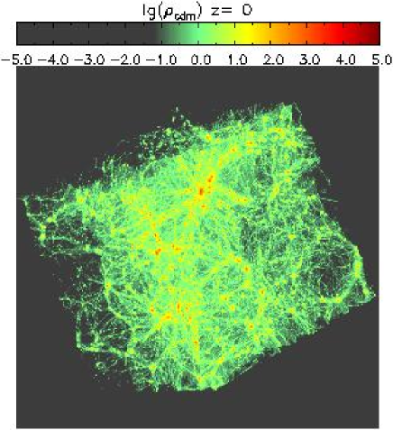
Figure 1: 3-D distribution of density fields of dark matter(left) and baryon(right) in a periodic box size of $25h^{-1}$ Mpc with a $512^{3}$ grid.

Figure 1 visualizes 3-D density distributions of the dark matter (left) and the baryon (right) respectively. Figure 2 gives the 3-D distributions of scalar field $\omega t$,$t$ is the cosmic time, at redshifts $z=4$, 2 and 0. The dimensionless quantity $\omega t$ is to characterize the typical number of eddy turnovers of vorticity within the cosmic time. Figure 2 shows a strong evolution of the intensity of vorticity with redshifts. The vorticity has not been well developed until redshifts $z\sim 4$, but becomes significant at $z\sim 2$ which marks approximately the onset of shocks and complex structures developed on the cosmic scales, and matches with the typical formation history of dark matter halos of galactic clusters (e.g. Bahcall & Fan 1998).

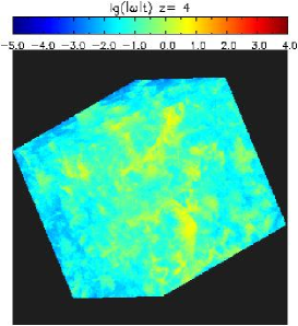
Figure 2: 3-D distribution of dimensionless scalar field $\omega t$ that refers to the number of turnovers of vortices within the cosmic time, where $t$ is the cosmic time, at redshifts $z=4$ (left), 2 (middle) and 0 (right).

The density fields (Figure 1) display the typical sheets-filaments-knot structures on the cosmic scale. However, the spatial configuration of the vorticity field looks quite different: it does not show any sheet-like or filamentary structure, instead, looks like clouds with the comparable sizes of clusters. Although the vorticity field is not associated with the fine structures of the underlying density fields, the cloudy structures are most likely to occur around overdense regions on large scales, and thus the vorticity field can be used to pick up the coherent structures. These features can be more clearly illustrated by 2-D distributions of $\omega t$ and vector projection of $\vec{\omega}$ shown in Figure 3, where a slide of $25\times 25\times 0.1$ $h^{-3}$ Mpc³ is taken. The distribution of $\vec{\omega}$ shows a similar spatial pattern as the scalar quantity $\omega t$.

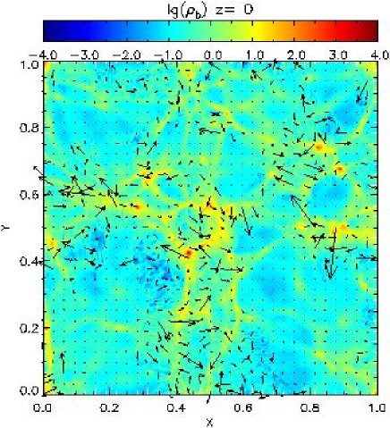
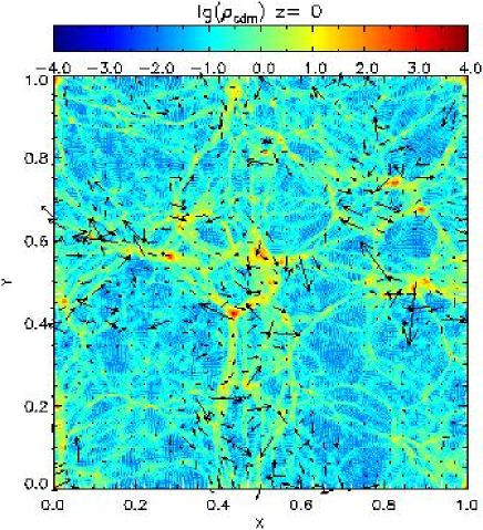
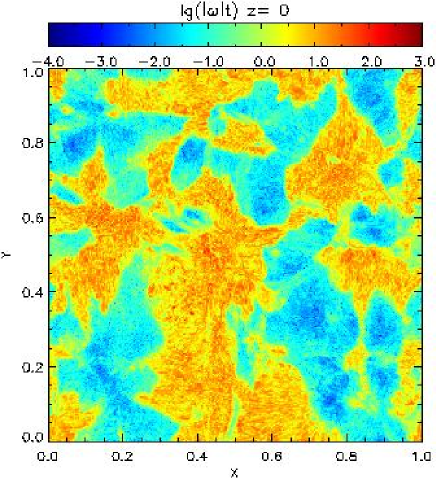
Figure 3: Vorticity in a slide of $25\times 25\times 0.1$ $h^{-3}$Mpc³. The top two plots give vector fields of $\vec{\omega}$ against background of baryon density(top left) and dark matter density(top right). The bottom left plot presents $\omega t$ in this slide while the baroclinity field is given by the bottom right panel.

It is recalled that, in a incompressible fluid, the evolution of vorticity is driven dominantly by the amplification of the strain rate term ${\bf S}\cdot{\vec{\omega}}$ [eq.(1)], which tends to stretch the vortical motion (Tanaka, & Kida, 1993; Constantin et al 1995) and produce filamentary(tubes) and/or sheetlike structure in the vorticity field (e.g. She et al 1990). As mentioned in §2.2, the strongest stretching is in the direction of $\vec{\xi}$, which is parallel to the eigenvector of tensor $\partial_{j}v_{i}$ with large positive eigenvalue. This mechanism distorts the vorticity field and forms a tube-like network in the spatial configuration.

The IGM, however, is compressible as a fluid. The amplification due to the strain rate ${\bf S}\cdot{\vec{\omega}}$ will be largely canceled by the term $-d\omega$ [eq.(2)], which results in a strong attenuation of vorticity in the direction parallel to the eigenvector of the tensor $\partial_{j}v_{i}$ with positive eigenvalues. Consequently, the vector field $\vec{\omega}$ does not show any clear sheetlike-filamentary structure.

Since vorticity is mostly attributed to the baroclinity $(1/\rho^{2})\nabla\rho\times\nabla p$, the distribution of vorticity should be determined by the distribution of baroclinity. In figure 3, we also present the baroclinity field in the same slide as that of $\omega t$. Clearly, both of them show alike structures. It is noted that, similar to the vorticity, the baroclinity can be strong even at low density regions, as shocks and complex structures can be formed there (He et al 2004).

Nevertheless, there does not exist a linear mapping between the $\omega t$ and the baroclinity. This is because the term $|\alpha\omega-d\omega|$ is sometimes comparable with the baroclinity $|(1/\rho^{2})\vec{\xi}\cdot(\nabla\rho\times\nabla p)|$. Figure 4 gives a cell-by-cell comparison between $|\alpha\omega-d\omega|$ and $|(1/\rho^{2})\vec{\xi}\cdot(\nabla\rho\times\nabla p)|$. In average, the intensity of these two sources are almost of the same order. Thus, the amplification and stretching by the rate-of-strain and divergence cannot be ignored. It leads to the mapping between the $\omega t$ and the baroclinity field deviating from a linear one.

Figure 4: A cell by cell comparison between the term $|\alpha\omega-d\omega|$, accounting for stretch in addition to expansion or contraction of vortices, and baroclinity $|(1/\rho^{2})\vec{\xi}\cdot(\nabla\rho\times\nabla p)|$, source of vorticity, at redshift $z=0$.

4.2 PDF of the Vorticity Fields

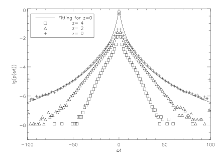
Figure 5: The probability distribution function (PDF) of vorticity $\vec{\omega_{i}}$ at redshifts $z=4$ (square), $z=2$ (triangle) and $z=0$ (cross).The solid line gives a log-normal fitting result for $z=0$.

We calculate the probability distribution function (PDF) of the three components of the vector field $\vec{\omega_{i}}$ at redshifts $z=4$, 2, 0. Giving that the vorticity field is isotropic, the PDFs of its three components $\vec{\omega_{i}}$, $i=x,y,z$ should be statistically identical, which is justified in our samples. We take an average over these three components at these redshifts and give the results in Figure 5. The PDF at present epoch exhibits a long tail, and can be approximately fitted by a log-normal distribution as

$$p(\omega t)d(\omega t)=\frac{1}{\omega t\sqrt{2\pi\sigma^{2}}}\exp\left[-\frac{1}{2}\left(\frac{\ln\omega t-\mu}{\sigma}\right)^{2}\right]d(\omega t)$$ (6)

where the variance $\sigma=0.98,\mu=0.37$, which implies that the vorticity field is intermittent, i.e. the probabilities of forming big vortical structures are much larger than Gaussian fields.

It shows that the PDF of vorticity fields has been always non-Gaussian since redshift $z\sim 4$, which is remarkably different from the velocity field of the IGM. The PDF of the velocity and pairwise velocity fields of dark matter and the IGM are Gaussian at high redshifts, corresponding to the linear phase of evolution (Yang, et al 2001). The evolution of the IGM vorticity field does not undergo a linear and Gaussian phase over cosmic times, since the vorticity can only be produced via nonlinear evolution. In this sense, the vorticity field is more effective than the velocity field to track the nonlinear evolution of the IGM.

Another interesting feature indicated in Figure 5 is that the PDF at high redshifts is approximately of exponential, and evolves into log-normal distribution at later phase. Thus, the PDF at different redshifts cannot be converted to each other by a scaling transformation. It implies that the turbulence experiences a strong nonlinear evolution, which will be revisited in next subsection.

4.3 Power Spectra of Velocity and Vorticity Fields

In a statistically homogeneous fluid, one can define the spectrum tensors $\Phi_{ij}({\bf k})$ and $\Omega_{ij}({\bf k})$ as the Fourier counterparts of the two-point correlation tensors of velocity $\langle v_{i}({\bf x+r})v_{j}({\bf x})\rangle$ and vorticity $\langle\omega_{i}({\bf x+r})\omega_{j}({\bf x})\rangle$,

$$\Phi_{ij}({\bf k})=\frac{1}{(2\pi)^{3}}\int\langle v_{i}({\bf x+r})v_{j}({\bf x})\rangle e^{-i{\bf k}\cdot{\bf r}}d{\bf r}$$ (7)

$$\Omega_{ij}({\bf k})=\frac{1}{(2\pi)^{3}}\int\langle\omega_{i}({\bf x+r})\omega_{j}({\bf x})\rangle e^{-i{\bf k}\cdot{\bf r}}d{\bf r}.$$ (8)

respectively, where $\langle...\rangle$ denotes average over spatial coordinates ${\bf x}$.

For a homogeneous turbulence, we have (Batchelor, 1959)

$$\Omega_{ij}({\bf k})=[\delta_{ij}k^{2}-k_{i}k_{j}]\Phi_{ll}({\bf k})-k^{2}\Phi_{ij}({\bf k}),$$ (9)

and hence,

$$\Omega_{ii}({\bf k})=k^{2}\Phi_{ii}({\bf k}).$$ (10)

The power spectra of velocity and vorticity fields are defined respectively as

$$P_{v}(k)=\int\frac{1}{2}\Phi_{ii}({\bf k})\delta(|{\bf k}|-k)d{\bf k};\hskip 8.53581ptP_{\omega}(k)=\int\frac{1}{2}\Omega_{ii}({\bf k})\delta(|{\bf k}|-k)d{\bf k}.$$ (11)

Combining eqs. (10) and (11) yields

$$P_{\omega}(k)=k^{2}P_{v}(k).$$ (12)

This relation is an important property of homogeneous turbulence (Batchelor, 1959), and can be used to measure the developed level of turbulence. If the velocity and vorticity fields of a fluid satisfy the relation given by eq.(12), it should be in the state of fully developed homogeneous turbulence. Otherwise, it would be less developed.

Figure 6: The power spectra $P_{\omega}(k)$ and $k^{2}P_{v}(k)$ at redshifts $z=4$ (top left), 2 (top right ) and 0 (bottom left) from $512^{3}$ simulation. The bottom right plot gives a resolution comparison of these two terms at redshift $z=0$.

Figure 6 compares the power spectra $P_{\omega}(k)$ with $k^{2}P_{v}(k)$ at $z=4$ (top left), 2 (top right) and 0 (bottom left), respectively. It shows that at high redshift $z=4$, the power spectrum $P_{\omega}(k)$ is much less than $k^{2}P_{v}(k)$ at almost all scales, which means that not all, actually only a small part, of the fluctuations of velocity field can be related to the random field of vorticity, and the turbulence is less developed by that time. While evolving to redshift $z\sim 2$, the turbulence is developed starting from the small scale 0.2$h^{-1}$ Mpc and up to 0.8$h^{-1}$ Mpc. At the present time, $z=0$, the turbulence is fully developed and extended to the scale 3$h^{-1}$Mpc, the typical scale of a cluster. The deviations of $P_{\omega}(k)$ from $k^{2}P_{v}(k)$ on scales less than 0.2 $h^{-1}$ Mpc are probably due to the energy dissipation of turbulence to thermal energy, or the virialization, on small scales. A panel of these two terms in the simulation run of lower resolution, $256^{3}$, is also presented in Fig. 6 and provides a convergence test of the resolution effect. It shows that the resolution does affect the lower end of turbulent scale as a result of dissipation. However, the turbulence on large scale is resolution converged.

Figure 6 also shows that the variance of velocity field on large scales is remarkably larger than that of vorticity field, especially at high redshifts. It indicates that the variance on large scales is not from the turbulent motion of the IGM and probably from bulk motion, which is due mainly to the falling into gravitational well. Therefore, to identify the variance of a velocity field as the signature of turbulence (e.g. Iapichino & Niemeyer 2008) may be questionable even on scales of clusters, as they generally contain many substructures at redshifts less than 2.

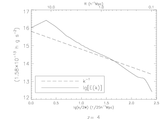
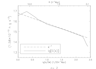
Figure 7: The power spectrum of kinetic energy(solid line) at redshifts $z=4$ (left), $2$ (middle) and $0$ (right). A power law $k^{-1}$ (dashed line) is used to fit the power spectrum.

We can also explore the evolution of turbulence with the spectrum of mean kinetic energy density $E(k)$ defined by $\int_{0}^{\infty}E(k)dk=1/2\langle\rho({\bf r})v^{2}({\bf r})\rangle$. The energy spectra $E(k)$ at redshifts $z=4$, 2 and 0 are shown in Figure 7. The energy spectra can be approximately fitted by a power law $k^{-\alpha}$ with $\alpha=1$ in the scale range of 0.15 - 3 $h^{-1}$ Mpc for $z=2$ and 0.15 - 10 $h^{-1}$ Mpc for $z=0$. These scale ranges are larger than that given by the power spectrum of velocity and vorticity. This is probably because the turbulent flow is strong in high density areas. Figure 7 shows that the energy spectrum becomes very steep at scales less than 0.15 $h^{-1}$ Mpc because of the dissipation on small scales. The energy spectrum at $z=4$ cannot be fitted with the power law of $k^{-1}$. It indicates that turbulence has not yet developed by then. Turbulence is effective at transferring kinetic energy on large scales to small one. Therefore, it leads to the power spectrum at $z<4$ to be more flat than that of $z=4$.

5 Effects of Turbulent IGM on Structure Formation

5.1 Non-thermal Pressure

An early attempt of including the effect of turbulent motions into gravitational collapsing processes was made by Chandrasekhar (1951). In his quantitative theory, he investigated the effect of micro turbulence in the subsonic regime. If turbulence is statistically homogeneous, it will contribute an extra pressure $p_{tub}=\rho\langle v^{2}\rangle$ on large scales. In the linear regime, Chandrasekhar derived a dispersion relation by introducing an effective sound speed $c^{2}_{s,eff}=c_{s}^{2}+(1/3)\langle v^{2}\rangle$ where $\langle v^{2}\rangle$ is the rms velocity dispersion due to turbulent motion. Obviously, the turbulence will slow down, or even halt the gravitational collapsing.

Chandrasekhar’s result had been improved by a more elaborate investigation (Bonazzola et al. 1992) , in which the scale dependence of the turbulent energy was taken account in the analysis of system instability. Actually, the gravitational instability on a scale $R$ will not be affected by fluctuation modes with wavelengths larger than $R$, and the fluctuation of velocity on the scales $k<2\pi/R$ do not contribute to the turbulent pressure for resisting on gravitational collapsing on scales that larger than $R$. Quantitatively, the turbulent pressure on the scale $R$ can be estimated by (Bonazzola et al 1987)

$$p_{tur}(k_{R})=\int_{k_{R}}^{k_{max}}E(k)dk,$$ (13)

where $E(k)$ is the turbulent power spectrum, $k_{R}=2\pi/R$, and ${k_{max}=2\pi/l_{diss}}$ is the wavenumber corresponding to the minimal scale $l_{diss}$ below which the turbulence decays due to energy dissipation or virialization.

According to the results presented in §4.3, the turbulence is fully developed on scales from 0.2 $h^{-1}$ Mpc up to 3 $h^{-1}$ Mpc since redshift $z\sim 2$. The direct outcome of the turbulence on those scales is expected to alter significantly the hydrostatic equilibrium state of the IGM or the process of structure formation. The turbulent pressure $p_{tur}(k_{R})$ as a function of $k_{R}$ is shown in Figure 8, where $l_{diss}=0.2$h^-1Mpc inferred from the power spectrum analysis in §4. 3. In practical calculation, since the energy spectrum $E(k)$ declines fast beyond 0.2 $h^{-1}$ Mpc (Fig. 7), one can take $k_{max}$ going to infinity safely. Since we have approximately $E(k)\propto k^{-1}$, $p_{tur}(k_{R})$ given by eq.(13) is weakly dependent on $k$. We also show the energy spectra $E(k)$ in Figure 8.

Using the power spectra measured in Figure 7, the turbulent pressure is estimated to be $1.5\times 10^{-17}$ g cm^-1s^-2 at $z=0$. According to $p/\rho=RT/\mu$, the effective temperature due to turbulent pressure is about $1.0\times 10^{6}$ K in regions of mean overdensity and $1.0\times 10^{5}$ K in regions of 10 time mean overdensity. Deduced from Ly$\alpha$ forests of quasars, the temperature of IGM at $\rho_{b}\simeq 1-10\rho_{b,0}$ is about $2\times 10^{4}$ K. Therefore, the nonthermal pressure of the turbulent flow could be larger than the thermal pressure of the IGM.

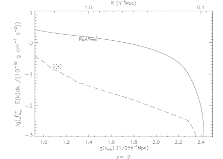
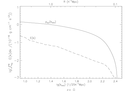
Figure 8: The spectrum of turbulent pressure $p_{tur}(k_{min})$, given by $p_{tur}(k_{min})=\int_{k_{min}}^{k_{max}}E(k)dk$, at redshifts $z=2$ (left) and $z=0$ (right). The energy spectra $E(k)$ are also shown in each panel.

The scale-dependence of the turbulent pressure is very weak. A decrease of one order of magnitude in scales from $R=3$ to $0.3$ $h^{-1}$ Mpc can only lead to deceases in the pressure $p_{tur}$ by a factor of 4. On the other hand, the mass $m$ of a cluster is related to its scale radius $r_{s}$ approximately as $m\propto r_{s}^{3}$ (Cooray & Sheth, 2002). The gravitational potential of $m$ halos at $r_{s}$ is $Gm/r_{s}\propto r_{s}^{2}$. Therefore, the ratio of the turbulent pressure to the gravitational potential at $r_{s}$ would be larger for clusters with smaller mass $m$. The effect of turbulent pressure on gravitational collapsing of baryon gas would be more significant on smaller clusters.

Figure 9: The distribution of $\ln(\omega^{2}/2S_{ij}S_{ij})$, which characterizes the net effect of turbulence on clustering and positive value represents prevention , in a 2-D slide of $25\times 25\times 0.1h^{-3}$ Mpc³ at redshift $z=2$ (left) and $0$ (right).

5.2 Vorticity and the Growth Rate of Velocity Divergence

In the nonlinear regime of the IGM gravitational clustering, the dynamical effect of turbulence can be estimated by eq.(3). Here, we are focusing on the first two terms from vorticity and strain rate. As discussed in §2.2, the net effect on the clustering is determined by the sign of quantity,

$$\frac{1}{2}\omega^{2}-S_{ij}S_{ij}=\frac{1}{2}[(\partial_{i}v_{j})(\partial_{i}v_{j})-3(\partial_{j}v_{i})(\partial_{i}v_{j})].$$ (14)

For a Gaussian velocity field, we have $\langle 3(\partial_{j}v_{i})(\partial_{i}v_{j})\rangle=\langle(\partial_{i}v_{j})(\partial_{i}v_{j})\rangle$, and in average, the net effect of velocity field in eq.(3) is statistically null. However, for a non-Gaussian velocity field, it can be either positive or negative, which is dependent on the property of the velocity field.

In homogeneous and isotropic turbulence, as $\langle(\partial_{j}v_{i})(\partial_{i}v_{j})\rangle=0$ (Batchelor 1959), the signs of Eq.(14) are always positive, which results in prevention of gravitational collapsing in the IGM. Figure 9 plots the spatial distribution of $\ln(\omega^{2}/2S_{ij}S_{ij})$ in the same simulation slide as that used in Figure 3. Comparing Figure 9 with Figures 3 , we find that all those cells with $\ln(\omega^{2}/2S_{ij}S_{ij})>0$ are located in the clouds around density peaks, where the vorticity is dominant. It provides a mechanism to prevent or slow down the IGM clustering with respect to the underlying dark matter.

We search for cells with $(1/2)\omega^{2}-S_{ij}S_{ij}>0$. At redshift $z=0$, there is a fraction $7.6\%$ of volume, $16.6\%$ of mass, with positive values of $(1/2)\omega^{2}-S_{ij}S_{ij}$, while at redshift $z=2$, this volume fraction has decreased down to $2.6\%$. Thus, the effect of turbulence becomes stronger to prevent the IGM clustering at lower redshifts.

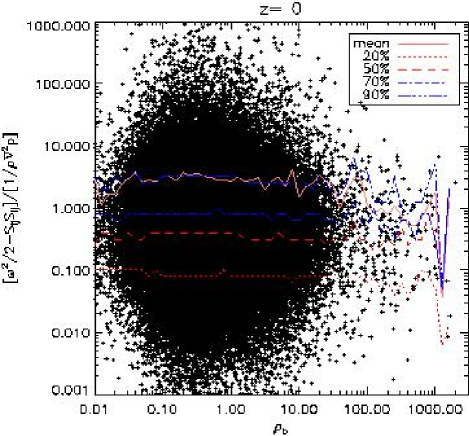
Figure 10: Comparison of effects of turbulent pressure and thermal pressure on the divergence $d$ (eq.(3)), $[\frac{1}{2}\omega^{2}-S_{ij}S_{ij}]/[\frac{1}{\rho}\nabla^{2}p]$, to baryon density of randomly selected cells with $\frac{1}{2}\omega^{2}>S_{ij}S_{ij}$ at redshift $z=0$. Solid line gives the mean value of this ratio at every density bin. Broken lines give the cumulative probability $20\%$,$50\%$,$70\%$ and $90\%$, from bottom to up.

In order to compare the effects of turbulent pressure and thermal pressure on the divergence $d$, we calculate the ratio of $(1/2)\omega^{2}-S_{ij}S_{ij}$ to $-\nabla^{2}p$ , taken from eq.(3), cell by cell. The result is presented in Figure 10, in which the cells are randomly selected from those with $\frac{1}{2}\omega^{2}>S_{ij}S_{ij}$ in the whole simulation samples. We find that for most densities nearly $30\%$ of those cells with $\frac{1}{2}\omega^{2}>S_{ij}S_{ij}$ have a value of this ratio larger than $1$ and indicate that mean turbulent pressure dominates over thermal pressure in them. Obviously, the dynamical prevention provided by turbulence could be comparable to that of thermal pressure and even become dominate in a considerable fraction of the whole volume.

6 Discussions and Concluding Remarks

The relationship between the fields of vorticity and velocity is similar to the relationship between the current of charge density and magnetic field, and thus, vorticity would be a measurement of the coherent spatial structures of velocity field. Moreover, the dynamical equation of vorticity is free from the gravitational field of dark matter and cosmic fluid. These remarkable features are very useful to study the nonlinear behavior of cosmic baryon fluid, especially the clustering behavior of the turbulent cosmic fluid in the gravitational field of underlying dark matter.

We show that the vorticity field of baryonic matter is significantly increasing with time when redshift $z\leq 2$. It can be understood that vorticity is effectively generated by shocks and complex structures of the baryon fluid, and then amplified by the rate-of-strain. At redshift $z=4$, the largest vorticity is only of the order of $\omega t\simeq 10$, while it is $\omega t\simeq 10^{2}$ at present universe. The IGM vorticity field is non-Gaussian and intermittent at all redshifts. The PDF of vorticity evolves from approximately exponential distributions at high redshifts to a distribution with log-normal long tail at present epoch.

The spatial configuration of the vorticity field is found to be very different from that of velocity and mass density. The distribution of vorticity does not follow the underlying matter structures, such as filaments and sheets. It always shows 3-D cloudy structures around gravitational collapsed regions, i.e. the knots in the filament-sheets structures. Even in regions surrounding high density structures, vorticity can be strong because complex structures, such as curved shocks and collision of shocks, are already formed around knots at their early phase of formation. Vorticity would be more effective to reveal the clustering behavior, which is overlooked by the mass density field in some way.

The fluctuations of vorticity field is useful to measure the development of a fully developed turbulence in the cosmic fluid. The relation between the power spectra of vorticity and velocity provides a measurement on the scale of velocity fluctuations where turbulence is fully developed. We find that the cosmic fluid is in the state of fully developed homogeneous and isotropic turbulence in the scale range of $0.2h^{-1}$Mpc to $3.0h^{-1}$Mpc at present epoch. With this result, we calculate the turbulent pressure. It is of the order of $1.5\times 10^{-17}$ g cm^-1s^-2 at $z=0$ in average, which is equivalent to the thermal pressure of gas with mean cosmic baryon density at temperature $1.0\times 10^{6}$ K. It tends to slow down the gravitational clustering of the baryon fluid. Moreover, the spectrum of turbulence pressure is weakly dependent on scale $k$, and then the effect of turbulent pressure would be relatively stronger on smaller objects.

The turbulent pressure may shed light on the problem of overcooling, i.e. the fraction of cold gas and stars in regions of galaxies, galaxies groups and clusters given by $\Lambda$CDM simulations is significantly higher than the observed value at $z\sim 0$ ( Nagai & Kravtsov, 2004, Crain et al. 2007, Keres et al. 2009). A possible way to solve this problem is to assume that the IGM undergo a pre-heating at low redshift (e.g. de Silva et al 2004). However, the pre-heating model is strongly in contradiction with the observations of the low-redshift Ly$\alpha$ forest of quasars, which cannot exist if the temperature of the IGM is $\geq 10^{5}$ K. Galactic winds is another mechanism proposed to suppress star formation in galaxies. Hydrodynamic simulations, however, suggest that such feedback would be inefficient in galaxies with $M_{gal}\geq 10^{9}M_{\odot}$(Mac Low & Ferrara 1999). Turbulent pressure essentially is dynamical and nonthermal. It can play the similar role as thermal pressure to prevent the gravitational clustering, while does not affect the thermal state and ionizing process of hydrogen in the IGM. The turbulent IGM can remain a temperature of $10^{4-5}$K and hence consistent with the observation of Ly$\alpha$ forest. If the IGM is turbulent, the Ly$\alpha$ absorption lines will not only show thermal broadening but also turbulent broadening. Observation of Ly$\alpha$ line widths of HI and HeII indicates that the broadening of Ly$\alpha$ forest is partially given turbulence broadening (Shull et al 2004, Zheng et al 2004, Liu et al 2006).

Vorticity enhances the transportation of mass, momentum and kinetic energy. The cascade of vortical structures leads to transfer of kinetic energy of vortical motion from large scales to small scales. The turbulence energy will further dissipate into thermal motion. This processes will enhance efficiently the entropy production via the thermalization and virialization. In addition, the turbulent motion can cause diffusive mixing of materials, which tends to wipe out gradients in the distribution of chemical composition. The details will be reported in the near future.

Appendix A The basic equations

A.1 Hydrodynamical equations for the IGM

The IGM is assumed to be an ideal fluid with polytropic index $\gamma$. The hydrodynamic equations for the IGM in the expanding universe can be written in the following form

$$\dot{U}+\partial_{i}f_{i}[U]=f(t,U)$$ (A1)

where $\partial_{i}\equiv\partial/\partial X_{i}$ ($i=1,2,3$), $X_{i}$ denote the proper coordinates, which are related to comoving coordinates $x_{i}$ by $X_{i}=a(t)x_{i}$, $a(t)$ being the scale factor. The quantity $U$ in eq.(A1) contains five components as

$$U=(\rho,\rho{\bf v},E)$$ (A2)

where $\rho$ is the comoving density of the IGM, ${\bf v}=\{v_{i}\}$ ($i=1,2,3$) are the peculiar velocity on three axes, $E=P/(\gamma-1)+\frac{1}{2}\rho{\bf v}^{2}$ is the total energy per unit comoving volume, $P=a^{3}p$, and $p$ is the pressure of the IGM. The quantities $f_{i}(U)$ in Eq.(A1) are given by the conservation laws of mass, momentum and energy as

$$f_{1}(U) = [\rho v_{1},\rho(v_{1})^{2}+P,\rho v_{1}v_{2},\rho v_{1}v_{3},v_{1}(E+P)]$$

$$f_{2}(U) = [\rho v_{2},\rho v_{1}v_{2},\rho(v_{2})^{2}+P,\rho v_{2}v_{3},v_{2}(E+P)]$$

$$f_{3}(U) = [\rho v_{3},\rho v_{1}v_{3},\rho v_{2}v_{3},\rho(v_{3})^{2}+P,v_{3}(E+P)]$$ (A3)

The ”force” term $f(t,U)$ on the right hand side of Eq. (A1) is given by

$$f(t,U)=(0,-\frac{\dot{a}}{a}\rho{\bf v}+\frac{1}{a}\rho{\bf g},-2\frac{\dot{a}}{a}E+\frac{1}{a}\rho{\bf v}\cdot{\bf g}-\Lambda_{rad}).$$ (A4)

The term of $-(\dot{a}/a)\rho{\bf v}$ is from the expansion of the universe. The term of $\Lambda_{rad}$ in Eq.(A4) is given by the radiative heating-cooling of the baryon gas. The gravitational force ${\bf g}=-\nabla\phi$ is produced by the matter including CDM and baryon , given by

$$\nabla^{2}\phi=\frac{4\pi G}{a}\bar{\rho}_{tot}\delta_{tot}.$$ (A5)

where the operator $\nabla$ acts on the comoving coordinate ${\bf x}$. $\delta_{tot}=[\rho_{tot}({\bf x},t)-\bar{\rho}_{tot}]/\bar{\rho}_{tot}$, and $\rho_{tot}$ is the total comoving mass density. Its mean value is $\bar{\rho}_{tot}(t)=1/6\pi Gt^{2}\propto a^{-3}$. The gravitational potential $\phi$ is zero (or constant) when the density perturbation $\delta_{tot}=0$.

A.2 Vorticity equation

Euler equation in comoving coordinates

$$\partial_{t}{\rho v_{i}}+\frac{1}{a}(\partial_{j}\rho v_{j}v_{i}+\partial_{j}\delta_{ij}P)=-\frac{\dot{a}}{a}\rho v_{i}+\frac{1}{a}\rho g_{i},$$ (A6)

or

$$\rho\partial_{t}{v_{i}}+v_{i}\partial_{t}\rho+\frac{1}{a}(v_{i}\partial_{j}\rho v_{i}+\rho v^{j}\partial_{j}v_{i}+\partial_{j}\delta_{ij}P)=-\frac{\dot{a}}{a}\rho v_{i}+\frac{1}{a}\rho g_{i},$$ (A7)

,where $\partial_{t}\equiv\partial/\partial t$. Therefore

$$\rho\partial_{t}{v_{i}}+\frac{1}{a}(\rho v_{j}\partial_{j}v_{i}+\partial_{j}\delta_{ij}P)=-\frac{\dot{a}}{a}\rho v_{i}+\frac{1}{a}\rho g_{i},$$ (A8)

or

$$\partial_{j}\delta_{ij}P\partial_{t}{v_{i}}+\frac{1}{a}v_{j}\partial_{j}v_{i}=-\frac{1}{a}(\frac{1}{\rho}\partial_{j}\delta_{ij}P+\dot{a}v_{i}-g_{i}).$$ (A9)

Using Levi Civita symbol

$$\epsilon_{ijk}\epsilon_{ilm}=\delta_{jl}\delta_{km}-\delta_{jm}\delta_{kl}$$ (A10)

we have

$$v_{j}\partial_{j}v_{i}=\frac{1}{2}\partial_{i}v_{j}v_{j}-\epsilon_{ijk}v_{j}\omega_{k},$$ (A11)

where $\omega_{i}=\epsilon_{ijk}\partial^{j}v_{k}$ is vorticity.

Taking operator of curl $\epsilon_{ijk}\partial^{j}$ on eq.(A9), we have term by term.

$$\epsilon_{ijk}\partial^{j}\partial_{t}{v_{k}}=\partial_{t}\epsilon_{ijk}\partial^{j}v_{k}=\partial_{t}\omega_{i}$$ (A12)

$$\epsilon_{ijk}\partial^{j}v_{l}\partial_{l}v_{k}=\epsilon_{ijk}\partial^{j}\frac{1}{2}\partial_{k}v_{l}v_{l}-\epsilon_{ijk}\partial^{j}\epsilon_{klm}v_{l}\omega_{m}$$ (A13)

$$\epsilon_{ijk}\partial^{j}\frac{1}{2}\partial_{k}v_{l}v_{l}=0$$ (A14)

$$\epsilon_{ijk}\partial^{j}\epsilon_{klm}v_{l}\omega_{m}=\epsilon_{kij}\epsilon_{klm}\partial^{j}v_{l}\omega_{m}=\partial^{m}v_{i}\omega_{m}-\partial^{l}v_{l}\omega_{i}=\omega_{m}\partial^{m}v_{i}-\omega_{i}\partial^{l}v_{l}-v_{l}\partial^{l}\omega_{i}$$ (A15)

Therefore, we have vorticity equation as

$$\partial_{t}\omega_{i}+\frac{1}{a}v_{l}\partial^{l}\omega_{i}=\frac{1}{a}(\omega_{m}\partial^{m}v_{i}-\omega_{i}\partial^{l}v_{l}+\frac{1}{\rho^{2}}\epsilon_{ijk}\partial_{j}\rho\partial_{k}p-\dot{a}\omega_{i}).$$ (A16)

Because $\omega_{i}(\partial^{j}v_{i}-\partial^{i}v_{j})=0$, we have

$$\partial_{t}\omega_{i}+\frac{1}{a}v_{l}\partial^{l}\omega_{i}=\frac{1}{a}(S_{ij}\omega_{j}-d\omega_{i}+\frac{1}{\rho^{2}}\epsilon_{ijk}\partial_{j}\rho\partial_{k}p-\dot{a}\omega_{i})$$ (A17)

where

$$S_{ij}=\frac{1}{2}(\partial^{j}v_{i}+\partial^{i}v_{j})$$ (A18)

and $d=\partial_{i}v_{i}$. In vector format

$$\partial_{t}{\bf\omega}+\frac{1}{a}{\bf v}\cdot{\nabla}\omega=\frac{1}{a}({\bf S}\cdot{\bf\omega}-d{\bf\omega}+\frac{1}{\rho^{2}}\nabla\rho\times\nabla p-\dot{a}\omega)$$ (A19)

A.3 Equation of divergence

Taking operator $\partial^{i}$ on eq.(A9), we have term by term,

$$\partial^{i}\partial_{t}{v_{i}}=\partial_{t}d$$ (A20)

$$\partial^{i}v_{j}\partial_{j}v_{i}=v_{j}\partial_{j}\partial^{i}v_{i}+(\partial^{i}v_{j})(\partial_{j}v_{i})=v_{j}\partial_{j}d+(\partial^{i}v_{j})(\partial_{j}v_{i})$$ (A21)

Using

$$\partial^{i}v_{j}=\frac{1}{2}(\partial^{i}v_{j}+\partial^{j}v_{i})+\frac{1}{2}(\partial^{i}v_{j}-\partial^{j}v_{i}),$$ (A22)

we have

$$(\partial^{i}v_{j})(\partial_{j}v_{i})=S_{ij}S_{ij}+\frac{1}{4}(\partial^{i}v_{j}-\partial^{j}v_{i})(\partial^{j}v_{i}-\partial^{i}v_{j})=S_{ij}S_{ij}+\frac{1}{2}\epsilon_{ijk}\partial_{j}v_{k}\epsilon_{ilm}\partial_{l}v_{m}.$$ (A23)

Therefore, the equation of divergence is

$$\partial_{t}d+\frac{1}{a}v_{l}\partial^{l}d=\frac{1}{a}(\frac{1}{2}\omega_{i}\omega_{i}-S_{ij}S_{ij}-\frac{1}{\rho}\partial_{i}\partial_{i}p+\frac{1}{\rho^{2}}\partial_{j}\rho\partial_{j}p-\dot{a}d-\frac{4\pi G}{a}(\rho-\rho_{0})).$$ (A24)

or in vector format

$$\partial_{t}d+\frac{1}{a}{\bf v}\cdot{\bf\nabla}d=\frac{1}{a}(\frac{1}{2}{\bf\omega}\cdot{\bf\omega}-S_{ij}S_{ij}-\frac{1}{\rho}\nabla^{2}p+\frac{1}{\rho^{2}}(\nabla\rho)\cdot(\nabla p)-\dot{a}d-\frac{4\pi G}{a}(\rho-\rho_{0})).$$ (A25)

A.4 A brief description of the numerical algorithm.

We use the fifth order finite difference WENO scheme (Jiang & Shu 2006) to demonstrate the basic idea of the WENO methodology. The fifth order WENO finite difference spatial discretization to a conservation law such as

$$u_{t}+f(u)_{x}+g(u)_{y}+h(u)_{z}=0$$ (A26)

approximates the derivatives, for example $f(u)_{x}$, by a conservative difference

$$f(u)_{x}|_{x=x_{j}}\approx\frac{1}{\Delta x}\left(\hat{f}_{j+1/2}-\hat{f}_{j-1/2}\right)$$ (A27)

along the $x$ axis, with $y$ and $z$ fixed, where $\hat{f}_{j+1/2}$ is the numerical flux. $g(u)_{y}$ and $h(u)_{z}$ are approximated in the same way. Hence finite difference methods have the same format for one and several space dimensions, which is a major advantage. For the simplest case of a scalar equation (A26) and if $f^{\prime}(u)\geq 0$, the fifth order finite difference WENO scheme has the flux given by

$$\hat{f}_{j+1/2}=w_{1}\hat{f}_{j+1/2}^{(1)}+w_{2}\hat{f}_{j+1/2}^{(2)}+w_{3}\hat{f}_{j+1/2}^{(3)}$$ (A28)

where $\hat{f}_{j+1/2}^{(i)}$ are three third order accurate fluxes on three different stencils given by

$$\hat{f}_{j+1/2}^{(1)}=\frac{1}{3}f(u_{j-2})-\frac{7}{6}f(u_{j-1})+\frac{11}{6}f(u_{j}),$$ (A29)

$$\hat{f}_{j+1/2}^{(2)}=-\frac{1}{6}f(u_{j-1})+\frac{5}{6}f(u_{j})+\frac{1}{3}f(u_{j+1}),$$ (A30)

$$\hat{f}_{j+1/2}^{(3)}=\frac{1}{3}f(u_{j})+\frac{5}{6}f(u_{j+1})-\frac{1}{6}f(u_{j+2}).$$ (A31)

Notice that the combined stencil for the flux $\hat{f}_{j+1/2}$ is biased to the left, which is upwinding for the positive wind direction due to the assumption $f^{\prime}(u)\geq 0$. The key ingredient for the success of WENO scheme relies on the design of the nonlinear weights $w_{i}$, which are given by

$$w_{i}=\frac{\tilde{w}_{i}}{\sum_{k=1}^{3}\tilde{w}_{k}},\qquad\tilde{w}_{k}=\frac{\gamma_{k}}{(\varepsilon+\beta_{k})^{2}},$$ (A32)

where the linear weights $\gamma_{k}$ are chosen to yield fifth order accuracy when combining three third order accurate fluxes, and are given by

$$\gamma_{1}=\frac{1}{10},\qquad\gamma_{2}=\frac{3}{5},\qquad\gamma_{3}=\frac{3}{10};$$ (A33)

the smoothness indicators $\beta_{k}$ are given by

$$\beta_{1} = \frac{13}{12}\left(f(u_{j-2})-2f(u_{j-1})+f(u_{j})\right)^{2}+\frac{1}{4}\left(f(u_{j-2})-4f(u_{j-1})+3f(u_{j})\right)^{2}$$ (A34)

$$\beta_{2} = \frac{13}{12}\left(f(u_{j-1})-2f(u_{j})+f(u_{j+1})\right)^{2}+\frac{1}{4}\left(f(u_{j-1})-f(u_{j+1})\right)^{2}$$ (A35)

$$\beta_{3} = \frac{13}{12}\left(f(u_{j})-2f(u_{j+1})+f(u_{j+2})\right)^{2}+\frac{1}{4}\left(3f(u_{j})-4f(u_{j+1})+f(u_{j+2})\right)^{2},$$ (A36)

and they measure how smooth the approximation based on a specific stencil is in the target cell. Finally, $\varepsilon$ is a parameter to avoid the denominator to become 0 and is usually taken as $\varepsilon=10^{-6}$ in the computation. There are no other parameters needed to be tuned by the user in the WENO method.

Meanwhile, the time step in simulation is set to the minimum value among two time scales. One is given by Courant condition as

$$\Delta t_{cfl}\leq\frac{CFL[a(t)\Delta x]}{max(|v_{1}+c_{s},v_{2}+c_{s},v_{3}+c_{s})},$$ (A37)

where $\Delta x$ is the cell size, $c_{s}$ is the local sound speed, $v_{1}$, $v_{2}$, and $v_{3}$ are fluid velocities, and CFL is the Courant number, here $CFL=0.60$. The other one is from cosmic expansion, which requires that $\Delta a/a<0.02$ within a single time step.

The WENO scheme is proven to be uniformly fifth order accurate including at smooth extrema, and this is verified numerically. Near discontinuities the scheme produces sharp and non-oscillatory discontinuity transition. The approximation is self-similar. Namely, when fully discretized with the Runge-Kutta methods, the scheme is invariant when the spatial and time variables are scaled by the same factor. This is a major advantage for approximating conservation laws which are invariant under such scaling.

References

- (1)
- (2) Bahcall, N. A., & Fan, X.H., 1998, ApJ, 504, 1
- (3)
- (4) Balsara, D., & Shu, C.-W., 2000, J. Comput. Phys., 160, 405
- (5)
- (6) Batchelor, G.K. 1959, The Theory of Homogeneous Turbulence, (Canbridge University Press)
- (7)
- (8) Benzi, R., Biferale, L. & Trovatore, E., 1996, Phys. Rev. Lett. 77, 3114
- (9)
- (10) Binney, J. 1974, MNRAS, 168, 73
- (11)
- (12) Bonazzola, S., Falgarone, Heyvaerts, J., Perault, M. & Puget, J. 1987, A&A, 172, 293
- (13)
- (14) Bonazzola, S., Perault, M., Puget, J., Heyvaerts, J., Falgarone, E. & Panis, J. 1992, J. of Fluid Mech. 245, 1
- (15)
- (16) Cassano, R. 2009, ASPC, 407, 223
- (17)
- (18) Carrillo, J. A., Gamba, I. M., Majorana, A., & Shu, C.-W. 2003, J. Comput. Phys., 184, 498
- (19)
- (20) Chandrasekhar, S. 1951a, Proc. Roy. Soc. A210, 18
- (21)
- (22) Chandrasekhar, S. 1951b, Proc. Roy. Soc. A210, 26
- (23)
- (24) Constantin. P., Procaccia, I., & Segel, D. 1995, PRE, 51, 3207
- (25)
- (26) Cooray, A., & Sheth, R., 2002, Physics Reports, 372, 1
- (27)
- (28) Crain. R. A., Eke V. R., Frenk C. S., Jenkins A., McCarthy I. G., Navarro J. F., & Pearce F. R., 2007, MNRAS, 377, 41
- (29)
- (30) Davis, G., & Widrow, L.M. 2000, ApJ, 540, 755
- (31)
- (32) de Silva, A,C., Kay, S.T., Lidde, A. R. & Thomas, P. A. 2004, MNRAS, 348, 1401
- (33)
- (34) Del Zanna, L., Velli, M., & Londrillo, P. 1998, A&A, 330, L13
- (35)
- (36) Dolag, K., Vazza, F., Brunetti G., & Tormen G. 2005, MNRAS, 364, 753
- (37)
- (38) Dubrulle, B. 1994, Phys. Rev. Lett. 73, 959
- (39)
- (40) Feng, L.L., Shu, C.-W., & Zhang, M.P. 2004, ApJ, 612, 1
- (41)
- (42) He, P., Feng, L.L., & Fang, L.Z. 2004, ApJ, 612, 14
- (43)
- (44) He, P., Feng, L.L., & Fang, L.Z. 2005, ApJ, 623, 601
- (45)
- (46) He, P., Liu, J., Feng, L.L., Shu, C.-W., & Fang, L.Z. 2006, Phys. Rev. Lett, 96, 051302
- (47)
- (48) Iapichino, L., & Niemeyer, J. C. 2008, MNRAS, 338, 1089
- (49)
- (50) Jiang, G. & Shu, C.-W, 2006, J. of Comput Phys, 126, 202
- (51)
- (52) Keres, D., Katz, N., Dav , R., Fardal, M., & Weinberg, David H., 2009, MNRAS, 396, 2332
- (53)
- (54) Kolmogorov, A. N. 1941, Dokl. Akad. Nauk. SSSR, 30, 301
- (55)
- (56) Komatsu, E., et al. 2009, ApJS, 180, 330
- (57)
- (58) Landau, L., & Lifshitz, E. 1959, Fluid Mechanics, (Pergamon Press)
- (59)
- (60) Liang, S., & Chen, H. 1999, AIAA J., 37, 1010
- (61)
- (62) Liu, J.R., Jamkhedkar, P., Zheng, W., Feng, L.L., & Fang, L.Z. 2006, ApJ, 645, 861
- (63)
- (64) Liu, J.R., & Fang, L.Z. 2008, ApJ, 672, 11
- (65)
- (66) Lu, Y., Chu, Y.Q., & Fang, L.Z. 2009, ApJ, 691, 43
- (67)
- (68) Mac Low M.-M., Ferrara A., 1999, ApJ, 513, 142
- (69)
- (70) Nagai, D., Kravtsov, A. V., 2004, Proceedings IAU Colloquium No. 195
- (71)
- (72) Pichon, C. & Bernardeau, F. 1999 A&A 343, 663
- (73)
- (74) Ryu, D., Kang, H., Cho, J., & Das, S. 2008, Science, 320, 909
- (75)
- (76) She, Z.S., Jackson, E., & Orsazg, S.A. 1990, Nature, 344, 226
- (77)
- (78) She, Z.S., & Leveque, E. 1994, Phys. Rev. Lett. , 72, 336
- (79)
- (80) She, Z.S. & Waymire, E.C., 1995, Phys. Rev. Lett. 74, 262
- (81)
- (82) Shi, J., Zhang, Y.T., & Shu, C.-W. 2003, J. Comput. Phys., 186, 690
- (83)
- (84) Shu, C.-W. 1998, in Lecture Notes in Mathematics, volume 1697, 325, (Springer).
- (85)
- (86) Shu, C.-W. 1999, in Lecture Notes in Computational Science and Engineering, volume 9, 439 (Springer).
- (87)
- (88) Shull, M. I., Tumlinson, J., Giroux, M. L., Kriss, G. A., & Reimers, D. 2004, ApJ, 600, 570
- (89)
- (90) Schmidt, W. 2007, arXiv:0712.0954v1
- (91)
- (92) Tanaka, M., & Kida, S. 1993, Physics of Fluids, 5, 2079
- (93)
- (94) Theuns, T., Leonard, A., Efstathiou, G. ,Pearce, F. R., & Thomas, P. A. 1998, MNRAS, 301,478
- (95)
- (96) Yang, X.H., Feng, L.L., Chu, Y.Q. & Fang, L.Z., 2001, ApJ, 560, 549.
- (97)
- (98) Zhang, S., Jiang, S., & Shu, C.-W. 2008, J. of Comp. Phys., 227, 7294
- (99)
- (100) Zhang, S., Jiang, S., Zhang, Y.-T., & Shu, C.-W. 2009, Phys. of Fluids, 21, 076101.
- (101)
- (102) Zhang, W.Q., Woosley, S.E., & MacFadyen, A. I. 2003, ApJ, 586, 356
- (103)
- (104) Zheng, W., et al. 2004, ApJ, 605, 631
- (105)