ELECTROMAGNETIC NON-CONTACT GEARS: PRELUDE

Abstract

We calculate the lateral Lifshitz force between corrugated dielectric slabs of finite thickness. Taking the thickness of the plates to infinity leads us to the lateral Lifshitz force between corrugated dielectric surfaces of infinite extent. Taking the dielectric constant to infinity leads us to the conductor limit which has been evaluated earlier in the literature.

1 Introduction

In past decade significant attention has been given to evaluation of the lateral force between corrugated surfaces (for example see Ref. Emig:2003,Chen:2002zz,Lambrecht:2008zz, CaveroPelaez:2008tj,CaveroPelaez:2008tk and references there-in). In an earlier work we calculated the contribution of the next-to-leading order to the lateral Casimir force between two corrugated semi-transparent $\delta$-function plates interacting with a scalar field [4], and the leading order contribution for the case of two concentric semi-transparent corrugated cylinders[5] using the multiple scattering formalism (see Ref. Milton:2007wz,Milton:2008st and references there-in). We observed that including the next-to-leading order contribution significantly reduced the deviation from the exact result in the case of weak coupling. Comparison with experiments requires the analogous calculation for the electromagnetic case. Here we present preliminary results of our ongoing work on the evaluation of the lateral Lifshitz force between two corrugated dielectric (non-magnetic) slabs of finite thickness interacting through the electromagnetic field (see Fig. 1).

From the general result it is easy to take various limiting cases. Taking the thickness of the dielectric slabs to infinity leads us to the lateral Lifshitz force between dielectric slabs of infinite extent. The lateral Casimir force between corrugated conductors was evaluated by Emig et al[1]. In our situation this is achieved by taking the dieletric constants $\varepsilon_{i}\rightarrow\infty$. Our results agree with the results in Emig et al[1]. Taking the thin-plate approximation based on the plasma model we have calculated the lateral force between corrugated plasma sheets. Our goal is to extend these results to next-to-leading order. Most of these will appear in a forthcoming paper.

2 Interaction energy

We consider two dielectric slabs of infinite extent in $x$-$y$ plane, which have corrugations in $y$-direction, as described in Fig. 1. We describe the dielectric slabs by the potentials

$$V_{i}(z,y)=(\varepsilon_{i}-1)\,\left[\theta(z-a_{i}-h_{i}(y))-\theta(z-b_{i}-h_{i}(y))\right],$$ (1)

where $i=1,2$, designates the individual dielectric slabs. $\theta(z)$ is the Heaviside theta function defined to equal 1 for $z>0$, and 0 when $z<0$. $h_{i}(y)$ describes the corrugations on the surface of the slabs. We define the thickness of the individual slabs as $d_{i}=b_{i}-a_{i}$, such that $a=a_{2}-b_{1}>0$ represents the distance between the slabs. The permittivities of the slabs are represented by $\varepsilon_{i}$.

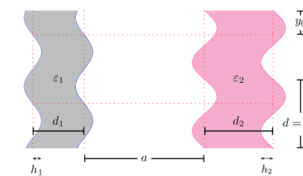
Figure 1: Parallel dielectric slabs with sinusoidal corrugations.

Using the multiple scattering formalism for the case of the electromagnetic field [8, 9] based on Schwinger’s Green’s dyadic formalism [10] and following the formalism described in Gears-I [4] we can obtain the contribution to the interaction energy between the two slabs in leading order in the corrugation amplitudes to be

$$E_{12}^{(2)}=\frac{i}{2}\,\int\frac{d\omega}{2\pi}\,\text{Tr}\left[\bm{\Gamma}^{(0)}\Delta V_{1}^{(1)}\cdot\bm{\Gamma}^{(0)}\,\Delta V_{2}^{(1)}\right],$$ (2)

where $\Delta V_{i}^{(1)}$ are the leading order contributions in the potentials due to the presence of corrugations. In particular, we have

$$\Delta V_{i}^{(1)}(z,y)=-h_{i}(y)\left(\varepsilon_{i}-1\right)\left[\delta(z-a_{i})-\delta(z-b_{i})\right].$$ (3)

Note that $V_{i}^{(0)}$ describes the potential for the case when the corrugations are absent and represent the background in the formalism. $\bm{\Gamma}^{(0)}=\bm{\Gamma}^{(0)}(\bm{x},\bm{x}^{\prime};\omega)$ is the Green’s dyadic in the presence of background potential $V_{i}^{(0)}$ and satisfies

$$\left[-\frac{1}{\omega^{2}}\bm{\nabla}\times\bm{\nabla}\times\;+\;\bm{1}+V_{1}^{(0)}+V_{2}^{(0)}\right]\cdot\bm{\Gamma}^{(0)}=-\bm{1}.$$ (4)

The corresponding reduced Green’s dyadic $\,\bm{\gamma}^{(0)}(z,z^{\prime};k_{x},k_{y},\omega)$ is defined by Fourier transforming in the transverse variables as

$$\bm{\Gamma}^{(0)}(\bm{x},\bm{x}^{\prime};\omega)=\int\frac{dk_{x}}{2\pi}\frac{dk_{y}}{2\pi}\,e^{ik_{x}(x-x^{\prime})}e^{ik_{y}(y-y^{\prime})}\,\bm{\gamma}^{(0)}(z,z^{\prime};k_{x},k_{y},\omega).$$ (5)

Using the fact that our system is translationally invariant in the $x$-direction, we can write

$$\frac{E_{12}^{(2)}}{L_{x}}=\int_{-\infty}^{\infty}\frac{dk_{y}}{2\pi}\int_{-\infty}^{\infty}\frac{dk_{y}^{\prime}}{2\pi}\,\tilde{h}_{1}(k_{y}-k_{y}^{\prime})\,\tilde{h}_{2}(k_{y}^{\prime}-k_{y})\,L^{(2)}(k_{y},k_{y}^{\prime}),$$ (6)

where $L_{x}$ is the length in the $x$-direction and $\tilde{h}_{i}(k_{y})$ are the Fourier transforms of the functions $h_{i}(y)$ describing the corrugations. The kernel $L^{(2)}(k_{y},k_{y}^{\prime})$ is given by

$$L^{(2)}(k_{y},k_{y}^{\prime})=-\frac{1}{2}\int\frac{d\zeta}{2\pi}\int\frac{dk_{x}}{2\pi}\,I^{(2)}(k_{x},\zeta,k_{y},k_{y}^{\prime}),$$ (7)

where

$$I^{(2)}(k_{x},\zeta,k_{y},k_{y}^{\prime}) = \left(\varepsilon_{a}-1\right)\left(\varepsilon_{b}-1\right)\hskip 113.81102pt$$ (8)

$$\times\Big{[}\,\bm{\gamma}^{(0)}(a_{2},a_{1};k_{x},k_{y},\omega)\cdot\bm{\gamma}^{(0)}(a_{1},a_{2};k_{x},k_{y}^{\prime},\omega)$$

$$\hskip 8.53581pt-\,\bm{\gamma}^{(0)}(b_{2},a_{1};k_{x},k_{y},\omega)\cdot\bm{\gamma}^{(0)}(a_{1},b_{2};k_{x},k_{y}^{\prime},\omega)$$

$$\hskip 8.53581pt-\,\bm{\gamma}^{(0)}(a_{2},b_{1};k_{x},k_{y},\omega)\cdot\bm{\gamma}^{(0)}(b_{1},a_{2};k_{x},k_{y}^{\prime},\omega)$$

$$\hskip 8.53581pt+\,\bm{\gamma}^{(0)}(b_{2},b_{1};k_{x},k_{y},\omega)\cdot\bm{\gamma}^{(0)}(b_{1},b_{2};k_{x},k_{y}^{\prime},\omega)\Big{]},$$

where the reduced Green’s dyadics are evaluated after solving Eq. (4). We note that $\bm{\gamma}^{(0)}(z,z^{\prime};k_{x},k_{y},\omega)={\bm{\gamma}^{(0)}}^{\dagger}(z^{\prime},z;k_{x},k_{y},\omega)$. Our task reduces to evaluating the reduced Green’s dyadic in the presence of the background. The details of this evaluation will be described in the forthcoming paper.

2.1 Evaluation of the reduced Green’s dyadic

The Green’s dyadic satisfies Eq. (4) whose solution can be determined by following the procedure decribed in Schwinger et al[10]. The expression for the reduced Green’s dyadic

$$\bm{\gamma}^{(0)}(z,z^{\prime};k,0,\zeta)=\left[\begin{array}[]{ccc}\frac{1}{\varepsilon(z)}\frac{\partial}{\partial z}\frac{1}{\varepsilon(z^{\prime})}\frac{\partial}{\partial z^{\prime}}\,g^{H}&0&\frac{ik}{\varepsilon(z^{\prime})}\frac{1}{\varepsilon(z)}\frac{\partial}{\partial z}\,g^{H}\\[8.53581pt] 0&-\zeta^{2}\,g^{E}&0\\[8.53581pt] -\frac{ik}{\varepsilon(z)}\frac{1}{\varepsilon(z^{\prime})}\frac{\partial}{\partial z^{\prime}}\,g^{H}&0&\frac{k^{2}}{\varepsilon(z)\varepsilon(z^{\prime})}\,g^{H}\end{array}\right]$$ (9)

is given in terms of the electric and magnetic Green’s functions $g^{E}(z,z^{\prime})$ and $g^{H}(z,z^{\prime})$, which satisfy the following differential equations:

$$-\left[\frac{\partial^{2}}{\partial z^{2}}-k^{2}-\zeta^{2}\varepsilon(z)\right]\,g^{E}(z,z^{\prime})=\delta(z-z^{\prime}),$$ (10)

$$-\left[\frac{\partial}{\partial z}\frac{1}{\varepsilon(z)}\frac{\partial}{\partial z}-\frac{k^{2}}{\varepsilon(z)}-\zeta^{2}\right]\,g^{H}(z,z^{\prime})=\delta(z-z^{\prime}).$$ (11)

We have used the definitions $k^{2}=k_{x}^{2}+k_{y}^{2}$ and $\varepsilon(z)=1+V_{1}^{(0)}(z)+V_{2}^{(0)}(z)$.

The reduced Green’s dyadic for arbitrary $k_{y}$ is generated by the rotation

$$\bm{\gamma}^{(0)}(z,z^{\prime};k_{x},k_{y},\zeta)=\mathbf{R}\cdot\bm{\gamma}^{(0)}(z,z^{\prime};k,0,\zeta)\cdot\mathbf{R}^{T},$$ (12)

where

$$\mathbf{R}=\frac{1}{k}\left(\begin{array}[]{ccc}k_{x}&-k_{y}&0\\ k_{y}&k_{x}&0\\ 0&0&k\end{array}\right).$$ (13)

We have dropped delta functions in Eq. (9) because they are evaluated at different points and thus do not contribute. We shall not present explicit solutions to the electric and magnetic Green’s functions here which will be presented in our forthcoming paper.

2.2 Interaction energy for corrugated dielectric slabs

Using the solutions to the electric and magnetic Green’s function in Eq. (9) we can evaluate $I^{(2)}(k_{x},\zeta,k_{y},k_{y}^{\prime})$ in Eq. (8) as

$$-\, \frac{1}{k^{2}}\frac{1}{{k^{\prime}}^{2}}\frac{1}{2\kappa}\frac{1}{2\kappa^{\prime}}\Bigg{[}\frac{1}{\Delta}\frac{1}{\Delta^{\prime}}M(-\alpha_{1},-\alpha_{1}^{\prime})M(-\alpha_{2},-\alpha_{2}^{\prime})(k_{x}^{2}+k_{y}k_{y}^{\prime})^{2}\zeta^{4}\hskip 85.35826pt$$

$$+\frac{1}{\Delta}\frac{1}{\bar{\Delta}^{\prime}}M(-\alpha_{1},\bar{\alpha}_{1}^{\prime})M(-\alpha_{2},\bar{\alpha}_{2}^{\prime})k_{x}^{2}(k_{y}-k_{y}^{\prime})^{2}\zeta^{2}{\kappa^{\prime}}^{2}\hskip 85.35826pt$$

$$+\frac{1}{\bar{\Delta}}\frac{1}{\Delta^{\prime}}M(\bar{\alpha}_{1},-\alpha_{1}^{\prime})M(\bar{\alpha}_{2},-\alpha_{2}^{\prime})k_{x}^{2}(k_{y}-k_{y}^{\prime})^{2}\zeta^{2}\kappa^{2}\hskip 85.35826pt$$

$$+\frac{1}{\bar{\Delta}}\frac{1}{\bar{\Delta}^{\prime}}\left\{M(\bar{\alpha}_{1},\bar{\alpha}_{1}^{\prime})(k_{x}^{2}+k_{y}k_{y}^{\prime})\kappa\kappa^{\prime}+M(-\bar{\alpha}_{1},-\bar{\alpha}_{1}^{\prime})k^{2}{k^{\prime}}^{2}\frac{1}{\varepsilon_{1}}\right\}\hskip 85.35826pt$$

$$\hskip 28.45274pt\times\left\{M(\bar{\alpha}_{2},\bar{\alpha}_{2}^{\prime})(k_{x}^{2}+k_{y}k_{y}^{\prime})\kappa\kappa^{\prime}+M(-\bar{\alpha}_{2},-\bar{\alpha}_{2}^{\prime})k^{2}{k^{\prime}}^{2}\frac{1}{\varepsilon_{2}}\right\}\Bigg{]},$$ (14)

where

$$\Delta = \big{[}(1-\alpha_{1}^{2}\,e^{-2\kappa_{1}d_{1}})(1-\alpha_{2}^{2}\,e^{-2\kappa_{2}d_{2}})\,e^{\kappa a}$$ (15)

$$\hskip 14.22636pt-\alpha_{1}\alpha_{2}(1-e^{-2\kappa_{1}d_{1}})(1-e^{-2\kappa_{2}d_{2}})\,e^{-\kappa a}\big{]},$$

$$M(\alpha_{i},\alpha_{i}^{\prime}) = (\varepsilon_{i}-1)\big{[}(1-\alpha_{i}^{2})\,e^{-\kappa_{i}d_{i}}(1-{\alpha_{i}^{\prime}}^{2})\,e^{-\kappa_{i}^{\prime}d_{i}}$$ (16)

$$\hskip 14.22636pt-(1+\alpha_{i})(1-\alpha_{i}\,e^{-2\kappa_{i}d_{i}})(1+\alpha_{i}^{\prime})(1-\alpha_{i}^{\prime}\,e^{-2\kappa_{i}^{\prime}d_{i}})\big{]},$$

where $\kappa_{i}^{2}=k^{2}+\zeta^{2}\varepsilon_{i}$, $\bar{\kappa}_{i}=\kappa_{i}/\varepsilon_{i}$, and $\alpha_{i}=(\kappa_{i}-\kappa)/(\kappa_{i}+\kappa)$. Quantities with primes are obtained by replacing $k_{y}\rightarrow k_{y}^{\prime}$ everywhere, and quantities with bars are obtained by replacing $\kappa_{i}$ with $\bar{\kappa}_{i}$ except in the exponentials.

2.3 Conductor limit

In the conductor limit ($\varepsilon_{i}\rightarrow\infty$) the above expression takes the form

$$I^{(2)}_{\varepsilon\rightarrow\infty}(\kappa,\kappa^{\prime},k_{y}-k_{y}^{\prime})=-\frac{\kappa}{\sinh\kappa a}\frac{\kappa^{\prime}}{\sinh\kappa^{\prime}a}\left[1+\frac{\{\kappa^{2}+{\kappa^{\prime}}^{2}-(k_{y}-k_{y}^{\prime})^{2}\}^{2}}{4\,\kappa^{2}{\kappa^{\prime}}^{2}}\right].$$ (17)

For the case of sinusoidal corrugations described by $h_{1}(y)=h_{1}\sin[k_{0}(y+y_{0})]$ and $h_{2}(y)=h_{2}\sin[k_{0}y]$ the lateral force can be evaluated to be

$$F^{(2)}_{\varepsilon\rightarrow\infty}=2k_{0}a\,\sin(k_{0}y_{0})\left|F^{(0)}_{\text{Cas}}\right|\frac{h_{1}}{a}\frac{h_{2}}{a}A^{(1,1)}_{\varepsilon\rightarrow\infty}(k_{0}a),$$ (18)

where

$$A^{(1,1)}_{\varepsilon\rightarrow\infty}(t_{0})=\frac{15}{\pi^{4}}\int_{-\infty}^{\infty}dt\int_{0}^{\infty}\bar{s}d\bar{s}\frac{s}{\sinh s}\frac{s_{+}}{\sinh s_{+}}\left[\frac{1}{2}+\frac{(s^{2}+s_{+}^{2}-t_{0}^{2})^{2}}{8\,s^{2}s_{+}^{2}}\right],$$ (19)

where $s^{2}=\bar{s}^{2}+t^{2}$ and $s_{+}^{2}=\bar{s}^{2}+(t+t_{0})^{2}$. The first term in Eq. (19) corresponds to the Dirichlet scalar case [4], which here corresponds to the E mode (referred to in Ref. Emig:2003 as TM mode). We note that $A^{(1,1)}_{\varepsilon\rightarrow\infty}(0)=1$. See Fig. 2 for the plot of $A^{(1,1)}_{\varepsilon\rightarrow\infty}(k_{0}a)$ versus $k_{0}a$. We observe that only in the PFA limit is the electromagnetic contribution twice that of the Dirichlet case, and in general the electromagnetic case is less than twice that of the Dirichlet case.

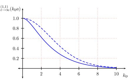
Figure 2: Plot of $A^{(1,1)}_{\varepsilon\rightarrow\infty}(k_{0}a)$ versus $k_{0}a$. The dotted curve represents 2 times the Dirichlet case.

Since the above expression involves a convolution of two functions we can evaluate one of the integrals to get

$$A^{(1,1)}_{\varepsilon\rightarrow\infty}(t_{0}) = \frac{15}{4}\int_{0}^{\infty}du\,\frac{\sin(2t_{0}u/\pi)}{(2t_{0}u/\pi)}\Bigg{[}\frac{\sinh^{2}u}{\cosh^{6}u}\left(\frac{7}{2}-\sinh^{2}u\right)$$ (20)

$$-\frac{1}{2}\left(\frac{2t_{0}}{\pi}\right)^{2}\frac{\sinh^{2}u}{\cosh^{4}u}+\frac{1}{16}\left(\frac{2t_{0}}{\pi}\right)^{4}\frac{\sinh^{2}u}{\cosh^{2}u}\Bigg{]},$$

which reproduces the result in Emig et al [1] apart from an overall factor of 2, which presumably is a transcription error. Even though Eq. (20) involves only a single integral it turns out that the double integral representation in Eq. (19) is more useful for numerical evaluation because of the oscillatory nature of the function $\sin x/x$ in the former.

3 Conclusion

We have evaluated leading order contribution to the lateral Lifshitz force between two corrugated dielectric slabs. Taking the dielectric constants of the two bodies to infinity gives the lateral Casimir force between corrugated conductors. We shall extend these results to next-to-leading order contribution for a better comparison with experiments in future publication as well as include various other limiting cases, which can be readily obtained from Eq.  (14).

References

- [1] T. Emig, A. Hanke, R. Golestanian and M. Kardar, Phys. Rev. A 67, 022114 (2003).
- [2] F. Chen, U. Mohideen, G. L. Klimchitskaya and V. M. Mostepanenko, Phys. Rev. A 66, 032113 (2002).
- [3] A. Lambrecht and V. N. Marachevsky, Phys. Rev. Lett. 101, 160403 (2008).
- [4] I. Cavero-Peláez, K. A. Milton, P. Parashar and K. V. Shajesh, Phys. Rev. D 78, 065018 (2008) [arXiv:0805.2776 [hep-th]].
- [5] I. Cavero-Peláez, K. A. Milton, P. Parashar and K. V. Shajesh, Phys. Rev. D 78, 065019 (2008) [arXiv:0805.2777 [hep-th]].
- [6] K. A. Milton and J. Wagner, J. Phys. A 41, 155402 (2008) [arXiv:0712.3811 [hep-th]].
- [7] K. A. Milton, J. Phys. Conf. Ser. 161, 012001 (2009) [arXiv:0809.2564 [hep-th]].
- [8] K. A. Milton, P. Parashar and J. Wagner, Phys. Rev. Lett. 101, 160402 (2008) [arXiv:0806.2880 [hep-th]].
- [9] K. A. Milton, P. Parashar and J. Wagner, in The Casimir Effect and Cosmology, ed. S. D. Odintsov, E. Elizalde, and O. B. Gorbunova, in honor of Iver Brevik (Tomsk State Pedagogical University), pp. 107-116 (2009) [arXiv:0811.0128 [math-ph]].
- [10] J. S. Schwinger, L. L. . DeRaad and K. A. Milton, Annals Phys. 115, 1 (1979).
- [11] K. A. Milton, The Casimir Effect: Physical Manifestations of Zero-Point Energy (World Scientific, Singapore, 2001).