Phenomenology of event shapes at hadron colliders
Abstract
We present results for matched distributions of a range of dijet event shapes at hadron colliders, combining next-to-leading logarithmic (NLL) accuracy in the resummation exponent, next-to-next-to leading logarithmic (NNLL) accuracy in its expansion and next-to-leading order (NLO) accuracy in a pure expansion. This is the first time that such a matching has been carried out for hadronic final-state observables at hadron colliders. We compare our results to Monte Carlo predictions, with and without matching to multi-parton tree-level fixed-order calculations. These studies suggest that hadron-collider event shapes have significant scope for constraining both perturbative and non-perturbative aspects of hadron-collider QCD. The differences between various calculational methods also highlight the limits of relying on simultaneous variations of renormalisation and factorisation scale in making reliable estimates of uncertainties in QCD predictions. We also discuss the sensitivity of event shapes to the topology of multi-jet events, which are expected to appear in many New Physics scenarios.
January 2010
1 Introduction
Event shapes measure the geometrical properties of the energy flow in QCD events and, notably, its deviation from that expected based on pure lowest order partonic predictions. Event shapes, as well as being among the first observables proposed to test QCD [1], have been inextricably tied with the progress of QCD. They have played a crucial role in the extraction of the strong coupling from properties of the final-state [2]. They have been essential in tuning the parton showers and non-perturbative components of Monte Carlo event generators [3, 4, 5, 6] and have also provided a laboratory for developing and testing analytical insight into the hadronisation process (e.g. refs. [7] and the reviews [8, 9]). From a technical point of view, the development of resummations and fixed-order calculations has benefited from comparisons of predictions for event-shape distributions obtained with both kinds of methods [10, 11, 12, 13, 14, 15, 16]. Additionally, they are one of the several tools that are used for classifying hadronic final states in new physics searches.
The majority of investigations of event shapes has been performed for colliders, with significant work also in DIS. A review of some of that work is given in [17]. In contrast, few dedicated studies have been performed on them at hadron colliders, with a handful of measurements at the Tevatron [18, 19, 20], a pure fixed order study [21], pure resummations in [22, 23, 24], and a recent experimental simulation study by CMS [25], as well as some investigation of the use of event shapes applied to jet contents for the identification of hadronic decays of boosted massive particles [26, 27, 28] (other approaches are reviewed e.g. in ref. [29]). The purpose of this article is to help bring our understanding of hadron-collider event-shape phenomenology closer to the level of sophistication that is standard in the and DIS cases, concentrating specifically on event shapes in hard QCD (dijet) events.
As is well known from the and DIS cases, accurate studies of event shapes involve the simultaneous use of two kinds of calculation. Fixed-order calculations provide expansions of event-shape distributions in powers of the strong coupling, . They are available up to next-leading-order (NLO) for hadron-collider event shapes, through the nlojet++ [21] program. When the event shape has a value , for each power of in the distribution there can be up two powers of a large logarithm, , associated with soft and collinear enhancements. This compromises the convergence of the perturbative series. The enhanced terms can however be resummed to all orders, providing the dominant contribution to the distribution for . Such resummed predictions tend to be carried out for the distribution integrated up to some value , which generally has an exponentiated structure . 111Not all event-shape distributions exponentiate, see e.g. [30, 31]. The term gives leading logarithmic (LL) accuracy in the exponent, is next-to-leading-logarithmic (NLL), etc. For suitable (recursively infrared and collinear safe, global) observables, the caesar program [31] calculates both and . To obtain a reliable prediction for an event shape distribution, one must combine both types of calculations, via a “matching” procedure [32]. An appropriately performed matching of NLO fixed order and NLL exponentiated resummation allows one to ensure that in the expansion of the resummation one correctly accounts for all terms , with , which is NNLL in the expansion. While NLO+NLL with NNLL in the expansion is the state-of-the-art for generic and DIS event shapes,222 For specific observables, higher logarithmic and/or fixed-order accuracies have been reached. This is e.g. the case with NNLL accuracy in the exponent for the energy-energy correlation [33], NNNLL for the thrust distribution in [15] and NNLL for the Higgs or vector boson transverse momentum spectrum at hadron colliders [34, 35]. Additionally NNLO accuracy has been achieved for a range of event shapes [14], with NNLO+NLL matching in [36] and NNLO+NNNLL in [15]. matching of this kind had not so far been achieved for hadron-collider event shapes.
Our study here will give NLL+NLO predictions for event shape distributions both at Tevatron (, TeV) and at the LHC (, TeV). We start in Sec. 2 by recalling the definitions of three classes of global event shapes for hadron colliders,333 For non-global observables [11], those sensitive to emissions only in a restricted phase space region, the angular-ordered branching underlying caesar’s resummations does not account for all NLL effects. Additional soft, large-angle contributions have to be resummed, which is currently possible only in the large- limit [11, 37] (though see also [38]). This is the reason why, in this work, we consider only the global case. addressing also the question of event shapes defined in terms of jets rather than particles. In Sec. 3 we describe the structure of the perturbative resummation as well as its matching to the NLO result. We also discuss possible general event-shape resummation issues associated with “super-leading” logarithms [39, 40]. In Sec. 4 we present our results for matched distributions, paying particular attention to the issue of theoretical uncertainties. We also compare our results to those obtained with parton-level shower Monte Carlo event generators, in some cases also matched to exact multi-parton tree-level matrix elements. In Sec. 5 we briefly discuss the impact of non-perturbative effects, the hadronisation and the underlying event. Finally, switching to more phenomenological questions, in Sec. 6 we compare various event shapes’ ability to distinguish characteristically different event topologies, and examine their robustness in such tasks, both with respect to parton showering and to the orientation of the final state event. Our results are summarised in Sec. 7. Some technical details are collected in Appendices A and B. Many further additional plots can be obtained from the URL [41].
2 Event-shape definitions at hadron colliders
In this article, we shall consider observables that measure the extent to which an event’s energy flow departs from a dijet structure. The lowest-order contribution to a dijet event consists of just two incoming and two outgoing partons. Throughout the paper we refer to these QCD configurations as the “Born limit”. Many of the event shapes studied here were presented for the first time in [23]. All share the property of continuous globalness [42, 31], which is a necessary condition for being able to carry out a resummation to NLL accuracy without a leading- approximation, and which also contributes to the simplicity of caesar’s generalised resummation approach (independently of the question of large- approximations). For an observable to be continuously global, it has to be sensitive to all emissions in an event (this is the requirement of globalness), and moreover it should have definite scaling properties with respect to secondary emission’s transverse momenta (see sec. 3.1.1 for a mathematical formulation). The continuously global event shapes we propose fall into three main classes: observables that are directly global, others that are supplemented with “exponentially suppressed forward terms” and observables with “recoil terms”.
2.1 Directly global observables
We first consider observables that are defined in terms of all hadrons in the event, therefore the name ‘directly’ global. The global transverse thrust is defined as
| (2.1) |
where the sum runs over all particles in the final state, represents the two momentum components transverse to the beam, its modulus, and is the transverse vector that maximises the sum. The observable which is resummed is then , which vanishes in the Born limit. The normalization of event shape observables to a hard transverse scale of the event is important because it reduces uncertainties associated with the experimental jet-energy scale, which partially cancel between numerator and denominator [43]. For most event shapes (except ) the choice of specific hard scale to which one normalises is arbitrary, and could for example also be the sum of the transverse momenta of the two hardest jets.
The transverse thrust axis and the beam form the so-called event plane. One can then define a directly global thrust minor, which is a measure of the out-of-event-plane energy flow
| (2.2) |
In close analogy with the case [44], one can formulate a transverse spherocity:
| (2.3) |
where the minimisation is carried over all possible unit transverse -vectors .444Numerically, the minimisation is simplified by the observation (based on extensive numerical tests) that the that provides the minimal sum always coincides with the transverse direction of one of the . This variable ranges from for pencil-like events, to a maximum of for circularly symmetric events.
An alternative observable, which makes use of a linearised version of the transverse momentum tensor (with direct analogy to the and parameters [45] used in ), is the -parameter:
| (2.4) |
where are the two eigenvalues of . Related variables have been considered in the plane transverse to the thrust axis in (resummed for -jet events in [46]) and in the plane transverse to a jet in the context of boosted top-quark decays [26, 28, 27], where forms involving the determinant of , e.g. , have been used. There is a one-to-one mapping between different forms, and we have chosen eq. (2.4) because it gives clearer separation between different kinematic regions.
Finally, we consider the exclusive variant of the -algorithm [47] (closely related to the inclusive variant [48] as adopted for Run II of the Tevatron [49] and expected to be used also at the LHC)
-
1.
One defines, for all final-state (pseudo)particles still in the event,
(2.5) and for each pair of final state particles
(2.6) where is the rapidity of particle and its azimuthal angle. The jet-radius parameter sets the angular reach of the jet algorithm. Throughout this paper, we will take .
-
2.
One determines the minimum over and of the and the and calls it . If the smallest value is then particle is included in the beam and eliminated from the final state particles. If the smallest value is then particles and are recombined into a pseudoparticle (jet). A number of recombination procedures exist. We adopt the E-scheme, in which the particle four-momenta are simply added together,
(2.7) -
3.
The procedure is repeated until only 3 pseudoparticles are left in the final state.
The observable we resum is the directly global three-jet resolution parameter
(2.8) where is defined by further clustering the event until only two jets remain and taking as the sum of the two jet transverse momenta,
(2.9)
While directly global event-shapes are defined in terms of all particles in the event, experimental measurements can be carried out only up to some given pseudorapidity ( at the Tevatron and at the LHC). However, as long as the event-shape’s value is not too small [22], , one can safely neglect the contribution of hadrons beyond the rapidity cut. The value up to which a NLL resummation is valid is observable specific. In particular, it depends on the behaviour of each event shape under a soft and collinear emission, as derived in [22, 23]. Further discussion is given in appendix B.
2.2 Observables with exponentially suppressed forward terms
One way to address the difficulty in performing measurements near the beam is to define event-shapes using only particles in a central region and to add a term sensitive to emissions along the beam direction, so as to render them global, but with an exponential suppression in the forward or backward directions. We define the central region by requiring that the rapidity of particles in satisfies , where specifies the rapidity region in which the two highest jets should lie, and is a rapidity buffer around the jets of size .
Given the central region , we introduce the mean transverse-energy weighted rapidity of this region,
| (2.10) |
and define the exponentially suppressed (boost-invariant) forward term as
| (2.11) |
We can then define non-global variants of the event-shapes defined in sec. 2.1 by restricting the sums to just the central region. For example, we have a central transverse thrust,
| (2.12) |
a central thrust minor
| (2.13) |
and a central three-jet resolution threshold, defined by the algorithm of section 2.1 applied only to the final state particles in (but maintaining the “beam” distance, eq. (2.5)).
Finally, we define “exponentially suppressed” variants of the event-shapes of sec. 2.1 by adding to the central event-shapes a power of which makes the event-shape continuously global [23]. We obtain the exponentially suppressed transverse thrust, thrust minor and three-jet resolution,
| (2.14) |
| (2.15) |
| (2.16) |
Additionally, one can consider event-shapes which are more naturally defined using particles only in a restricted region, like jet-masses and broadenings. Given a central transverse thrust axis , one can separate the central region into an up part consisting of all particles in with and a down part with respectively. One then defines, in analogy with [50], the normalised squared invariant masses of the two regions
| (2.17) |
from which one can obtain a (non-global) central sum of masses and heavy-mass,
| (2.18) |
and the corresponding global event-shapes, the exponentially-suppressed sum of masses and heavy-mass
| (2.19) |
With the same division into up and down regions as for the jet masses, one can define jet broadenings. To do so in a boost-invariant manner, one first introduces rapidities and azimuthal angles of axes for the up and down regions,
| (2.20) |
and defines broadenings for the two regions,
| (2.21) |
from which one can obtain central total and wide-jet broadenings,
| (2.22) |
Adding the forward term one obtains the global exponentially-suppressed total and wide-jet broadenings,
| (2.23) |
We note that an observable that effectively has exponentially suppressed forward behaviour has also been studied in [24].
2.3 Observables with recoil term (indirectly global observables)
Because of transverse momentum conservation, if radiation is emitted in the forward region , recoil effects will cause the vector sum of the transverse momenta in the complementary, central region to be non-vanishing. It is then possible to exploit this effect to make observables (continuously) global, despite the fact that only a central subset of particles in the event effectively enters the definition of the event shapes. To do so, we add to the central event-shapes a suitable power of a recoil term, the two-dimensional vector sum of the transverse momenta in ,
| (2.24) |
We obtain than recoil enhanced transverse thrust, thrust minor, three-jet resolution, sum- and heavy-jet masses, total and wide broadenings
| (2.25a) | ||||
| (2.25b) | ||||
| (2.25c) | ||||
| (2.25d) | ||||
| (2.25e) | ||||
2.4 Particles versus jets as inputs
The event shapes discussed so far have all been defined in terms of the particles in the event. The experiments don’t measure particles directly. They do, however, have methods such as the combination of information from electromagnetic and hadronic calorimeters into “Topoclusters” (ATLAS [51]) and, with tracking, “particle flow” (CMS [52]), that provide inputs to jet algorithms that are quite close to particles. These same inputs would probably also be well suited to event-shape studies.
In uses of event shapes to cut on event topology in beyond-standard-model searches, as well as in the study of ref. [25], it is not particles but instead jets that have been used as inputs. The jets are usually defined through an angular resolution parameter (as in eq. (2.6)) and a transverse momentum cutoff, which we will denote . One of the interests of using jets is that the cutoff eliminates much of the contamination from the underlying event, which can easily contribute of transverse momentum to the rapidity region covered by LHC detectors.
From the point of view of resummation, the use of jets as inputs poses two main problems. One comes from the presence of the new scale in the problem: in terms of the parameters and defining the event-shape’s sensitivity to radiation along the incoming legs (cf. table 1 and section 3.1.1), this new scale causes separate regions of event shape value to each involve different logarithmic structure: for cases with the potentially different regions are , and . The first of these regions may be within the scope of caesar if is sufficiently small.
A second problem is that of globalness. Emissions collinear to any outgoing hard parton will be clustered together with its emitter to form a jet. The observable’s sensitivity to these emissions will then depend on the jet recombination scheme. In the -scheme, the current default at the Tevatron and LHC, the jet four-momentum is constructed by simply adding the four momenta of its constituents. Therefore, all observables defined using transverse momenta will get no sensitivity to emissions inside each of the two hard jets, and will therefore be non-global. This statement is true for any recombination scheme that adds three-momenta vectorially. For variables with sensitivity to longitudinal degrees of freedom, globalness can only be assessed on a case by case basis. For instance if one considers any global version of the total and heavy-jet mass (with exponentially suppressed or recoil term), in the -scheme the mass of each central hard jet will enter the hemisphere central jet mass in eq. (2.17). Therefore one obtains the same result for the central component of the event shape as would have been obtained using hadrons as inputs (modulo the fact that the jet clustering may affect which particles are considered central).
One alternative to the use of jets as inputs, in order to avoid the globalness issue, is the following: use as inputs the particles that are inside the two hardest jets, together with all the remaining jet momenta. Note that this does not eliminate the issue of the extra scales related to , though it does maintain the reduced sensitivity to underlying event that comes from the use of jets.
3 Structure of the perturbative calculation
Typically one wishes to consider event shapes only for events that are sufficiently hard, requiring for example at least one jet above some minimum transverse momentum threshold and in some central rapidity region. We will denote this kind of hardness selection cut by a function of the particles in the event; is equal to for events that pass the cuts and otherwise. One can then define the cross section for events that pass the cuts,
| (3.1) |
where is the differential cross section for producing particles in some configuration . One can determine perturbatively as long as corresponds to an infrared and collinear (IRC) safe selection procedure.
One also defines the partial integrated cross section for events that pass the cut and for which additionally the event shape observable is smaller than some value ,
| (3.2) |
The differential normalised distribution for the event shape is then given by
| (3.3) |
Perturbatively we will write and as expansions in the number of powers of the coupling that they contain,
| (3.4) |
where is the leading order (LO) result, the NLO result, etc.; is proportional to . We have chosen not to extract the powers of from the coefficients, because the scale of may depend on the kinematics of the events over which one has integrated.
The expansion for is similar
| (3.5) |
with the property that because the observable vanishes at . looks like a NLO term in eq. (3.5), but it is usually determined from the LO term for the differential cross section of ,
| (3.6) |
The quantity is similarly determined from the NLO term of the differential cross section of . In the following we shall never use explicitly , since , the NNLO correction to the dijet cross section, has yet to be calculated and since its effect would lead to terms that are beyond our accuracy in differential distributions.
3.1 Resummation
Resummations are relevant in the region of small , where logarithmically enhanced contributions of soft and collinear origin, as large as , appear at all orders in the integrated cross section , thus making fixed-order predictions unreliable. There is a large class of observables for which one can write a common “master” resummation formula, as was done in [31], in order to sum such terms to all orders in . In this section we will first examine what the class of observables is, and then review the broad structure of the resummation.
3.1.1 Prerequisites for resummation with caesar
In order for an observable to be resummed within the caesar framework, its functional behaviour in the presence of an arbitrary number of soft and/or collinear emissions has to satisfy a number of conditions. These have been extensively discussed in [31], and are checked automatically by caesar given a computer subroutine that computes the value of the an observable given a set of four-momenta. The conditions are:
-
1.
a specific functional form for the observable’s dependence on the momentum of a single soft emission , collinear to one of the hard “Born” partons (“legs”) in the event:
(3.7) where denote the Born momenta (including recoil effects) and is the soft collinear emission; and denote respectively its transverse momentum and rapidity, as measured with respect to the Born parton (‘leg’) labelled ; is the azimuthal angle of the emission with respect to a suitably defined event plane (when relevant); can be any function for which is well defined; is a hard scale of the problem (taken here to be the sum of the transverse momenta of the two hardest jets).
-
2.
continuous globalness [11, 53], a requirement on the observable’s single-emission scaling properties in every region of the phase space. First, all the have to be equal, , and the have to be all non-zero. Second, the observable’s scaling at the boundaries of the soft collinear region has to be consistent with eq. (3.7), i.e. in the soft large-angle region we require for a fixed angle of , whilst for hard emission collinear to leg we must have at fixed energy for .
-
3.
recursive infrared and collinear safety, a subtle mathematical condition (see [31] for its precise formulation) concerning the observable’s scaling in the presence of multiple soft/collinear emissions.
Table 1 summarises the values of the coefficients and for the event shapes presented in section 2. We stress that central observables, like the central transverse thrust eq. (2.12), defined using only hadron momenta in a selected rapidity interval, tend to have , and therefore be non-global. [but not true for .] The exponentially-suppressed term in eq. (2.11) or the recoil term in eq. (2.24), as explained in sections 2.2 and 2.3, are added to central event shapes precisely so as to make them global. The different powers of and that appear in the definition of these modified event shapes (see for instance eqs. (2.14) and (2.16)) are chosen so as to ensure their continuous globalness. This can be seen by observing that, for each event shape, the coefficients corresponding to different legs are equal. This above discussion holds for most observables but there may be exceptions. For example, the central variant of the thrust-minor is actually a global observable because of an indirect sensitivity to non-central emissions due to recoil. This is the reason why the coefficients for are not those that usually appear for observables with exponentially-suppressed components, but are rather those typical of a (linear) recoil term.
| 1 | 0 | 1 | 1 | |
| 1 | 1 | 1 | 1 | |
| 1 | 1 | 1 | 0 | |
| 1 | 0 | 1 | 0 | |
| 1 | 0 | 1 | 0 | |
| 1 | 0 | 1 | 0 | |
| 2 | 0 | 2 | 0 | |
| 2 | 2 | 2 | 0 | |
| 2 | 0 | 2 | 0 | |
| 1 | 1 | 1 | 0 | |
| 1 | 0 | 1 | 0 | |
| 1 | 1 | 1 | 1 | |
| 1 | 0 | 1 | 1 | |
| 1 | 0 | 1 | 1 | |
| 2 | 0 | 2 | 0 |
Recursive infrared and collinear (rIRC) safety, a detailed discussion of which is beyond the scope of the present paper, is trivially satisfied for all observables that we discuss here.
3.1.2 NLL resummation structure
For global observables, in events with , it is possible, unambiguously, to associate the event kinematics with that of a (Born) event. This is because the requirement forces all radiation to be either soft or collinear. At perturbative level it is also possible to unambiguously attribute a partonic subprocess to the event, for example (doing so requires a flavour infrared and collinear safe procedure, as in [54], but the result is independent of the choice of the procedure). Here we will use to label the event’s kinematics and to label its flavour structure. Then we can write as a sum over partonic subprocesses and an integral over Born configurations that pass the hard event cuts,
| (3.8) |
The ambiguities in such a decomposition of are suppressed by powers of .
For observables that satisfy the properties of the previous section, the result of ref. [31] is that we can write
| (3.9) |
where is the LO cross section, differential in the Born configuration, separated into subprocesses, and understood to have been evaluated with a factorisation scale . The function encodes the resummation, and has the form [55, 32]
| (3.10) |
where , with some renormalisation scale of order .
The order-by-order expansion of involves terms of the form . It is because of the property of “exponentiation” (a consequence of rIRC safety and of coherence555The validity of coherence is brought into question by the findings of refs. [39, 40] and we discuss the possible implications of this in section 3.3. ) that one can write it in the form eq. (3.10), whose leading-logarithmic (LL) contribution in the exponent, , resums terms : i.e. corrections to the first order term involve only powers of . The function resums “next-to-leading logarithmic” (NLL) terms in the exponent, , also referred to sometimes as single-logarithmic terms.
The LL function can be computed analytically given only the and values. It is given by
| (3.11) |
where is the colour charge ( or ) of hard parton for the hard-scattering subprocess , and . Since the coefficients and do not depend on the particular momentum configuration of the hard partons, is also independent of . Its dependence on the subprocess arises only through the colour charges of the incoming and outgoing partons.
The NLL function can be decomposed into three types of terms [31]
| (3.12) |
The term accounts for NLL corrections associated with the event kinematics, the particular values of the and coefficients in eq. (3.7), the choice of renormalisation scale and scheme used in in , as well as the non-trivial colour evolution of large-angle soft virtual gluon resummation [56, 57, 58, 59, 60].
The second term on the right-hand side (RHS) of eq. (3.12) involves parton distribution functions (PDF) for the parton flavours in the initial state of the given subprocess, , at a longitudinal momentum fraction for each leg that depends on the Born kinematics. This term arises because the PDFs in in eq. (3.9) were evaluated at a factorisation scale . The presence of a PDF at scale implies that one integrates over all possible incoming collinear emissions, up to . However the requirement that the event shape be small, , restricts collinear emissions to have . Thus the PDFs should actually be evaluated at a factorisation scale (as occurs also in Drell-Yan transverse-momentum resummations [55, 61, 62]). The ratio of PDFs in eq. (3.12) serves to replace as used in the Born cross section with a PDF at the correct factorisation scale.
The third term on the RHS of eq. (3.12) accounts for the NLL corrections associated with the presence of multiple soft and collinear emissions, when each has and they are all widely separated in rapidity. It is a function of
| (3.13) |
and is known analytically for some observables (e.g. ), while in all other cases caesar can compute it numerically via a suitable Monte Carlo procedure. sometimes depends on the underlying scattering channel , but not (for the observables studied here) on the hard momentum configuration.
The behaviour of with increasing (decreasing ) is a characteristic feature of each event shape. It depends on whether multiple emissions tend to increase or decrease the value of the event shape. In the first case, for a fixed value , has to account for an extra suppression of emissions so as to keep the event shape’s value less than , i.e. . For the special case of then (for example the jet resolution threshold [12] in the Cambridge jet algorithm [63]). Conversely if the contributions of multiple emissions tend to cancel, the function has to compensate the excessive suppression given by the LL function , therefore .
This last case appears most dramatically when it is a cancellation between multiple emissions, and not a direct veto on real emissions, that is the dominant effect that keeps the event shape small. In this case the LL function (whose functional form depends only on the effect of single emission) no longer accounts for the dominant contribution to the distribution. Furthermore, no NLL function such as can fully compensate for this. This inconsistency reveals itself through a divergence of at a given critical value , which can be inferred from considerations on the cancellation mechanism, as explained in refs. [23, 31]. Such a divergence is present, for example, for and and occurs at , where and are the colour charges of incoming partons and the total colour charge of the hard parton system. It will prevent us from obtaining sensible NLL resummed results for these observables. In the case of recoil observables there is also a divergence, but at larger (smaller ), for example at for and . The effect on the corresponding differential distributions will be discussed when presenting matched results.
3.1.3 NNLLΣ accuracy
As well as discussing the LL, NLL, etc. accuracy of resummation in the exponent of eq. (3.10), one can also discuss the accuracy in the order by order expansion of itself. In this way of counting logarithms, “LLΣ” terms involve powers , NLLΣ involve , etc. A NLL resummation in the exponent automatically guarantees NLLΣ accuracy. However it is also possible (if not entirely straightforward), given the information at our disposal, to obtain NNLLΣ accuracy. To see how, observe that the terms that we neglect in eqs. (3.9) and (3.10) are an overall correction without logarithms, as well as terms in the exponent, starting at . The latter, if they multiply when expanding the exponent, lead at most to , i.e. they are NNNLLΣ. We can therefore ignore them. As for the overall correction, when multiplied by the double logarithms, it gives us terms , which are NNLLΣ and therefore cannot be neglected. This means that we need to determine the coefficient of the pure term.
To do so, let us define the NLL resummed cross section as
| (3.14) |
with containing only the LL and NLL resummation terms,
| (3.15) |
Then we can determine the coefficient in terms of the first order expansion of the exact and resummed distributions, and in particular their difference as ,
| (3.16) |
The constant involves many contributions, including parts that cancel the and dependence present in the Born cross section, parts that are sensitive the observable’s exact behaviour with respect to soft large-angle emission and hard collinear splitting and parts related to the exact structure of the 1-loop scattering diagram.
Now we can write the NNLLΣ resummed distribution as
| (3.17) |
The fact that we may multiply and in order to get NNLLΣ accuracy is a consequence of the property that soft-collinear virtual corrections, which give powers of , affect neither the flavour, the momentum nor the colour involved in the hard scattering or the PDFs and therefore straightforwardly multiply all the more complicated contributions that are present in .
In practice, it is not feasible to (numerically) determine the exact first order distribution for fully differentially in the Born configurations. Considering instead quantities , (and their order-by-order expansions), integrated over configurations that pass the event cuts, as in eq. (3.8), one can define a coefficient averaged over Born momentum configurations,
| (3.18) |
Writing
| (3.19) |
gives a distribution that is still correct to NNLLΣ accuracy, because the LL, , component of is independent of the momentum configuration.
In contrast, if one considers averaged additionally over subprocesses
| (3.20) |
then
| (3.21) |
is not accurate to NNLLΣ, because
| (3.22) |
since the coefficient of the double logarithms in does depend on the subprocess, through the colour charges of the hard partons.
3.2 Matching of NLL to NLO
While the resummation of logarithms is necessary in the region where event-shape values are small and their logarithms large, the region of large values of is dominated by events with three or more well separated jets. Those types of events are described more reliably by fixed order calculations. It has therefore become standard to match resummed calculations to next-to-leading order (NLO) to have a reliable prediction over a larger range of values of . In this section we will present the formulae we use to perform the matching.
In the following we will denote with the integrated event-shape fraction, where and are defined in eqs. (3.2) and (3.1) respectively. After a NLL+NLO matching this quantity should satisfy the following requirements
-
1.
it should respect the physical constraints that, when the event shape reaches its maximum value , we have exactly and ;
-
2.
its expansion up to relative should reproduce the exact NLO result for the corresponding differential distribution;
-
3.
one should obtain NNLLΣ accuracy, i.e. all logarithms with should be correctly accounted for, which implies that the matching formula should reduce to eq. (3.19) in the limit of small . Preferably this should be the case without having to go through the tedious procedure of manually determining separately for each event shape.
There are various matching procedures that satisfy these requirements and therefore formally have the same accuracy. We consider here the so-called log- [32] and multiplicative [42] matching schemes, adapted to hadron-hadron collisions. In particular both need to be modified in accordance with the need, section 3.1.3, to have the constant term multiply the resummation separately for each subprocess. Actually, what matters is not so much the subprocess but the colour charges of the incoming and the outgoing Born partons. Therefore we can consider all subprocesses , , , etc., with the same incoming and the same outgoing colour charges as belonging to a single colour channel . The other colour channels are , , and .666 We study here only observables whose double logarithms depend only on the total colour charge of the two incoming and two outgoing partons, so that we do not to distinguish incoming partons and (or outgoing partons and ). This means that for the matching only the colour structure is relevant, therefore this colour labelling does not distinguish quarks from anti-quarks or quarks of different flavour. A given colour channel is then in general a sum over multiple partonic channels .
We denote by the expansion of the resummed cross section corresponding to a specific colour channel and by the corresponding exact fixed order prediction. In analogy with eq. (3.8), where the index is omitted a sum over all possible colour channels is understood. The index denotes the order in of the expansion (relative to the Born cross section).
We have obtained fixed order cross-sections using the code nlojet++ [21]. The publicly available version computes cross-sections summed over the flavour of outgoing partons. We therefore extended it so as to have access to the flavour of both incoming and outgoing partons in the calculation of , and , though not for since its colour-channel separation is not needed for NNLLΣ accuracy. To assign events with more than two outgoing partons to a definite colour channel we used the exclusive flavour- algorithm of [54] to cluster events to a topology while keeping track of flavour in an infrared safe manner. During the clustering procedure, quarks of different flavour might end up in the same jet, giving rise to multi-flavoured jets, i.e. jets whose flavour does not correspond to any QCD parton. These events, which do not correspond to any Born processes and have vanishing weights for , will be labelled as having .
The matching equations are defined in terms of the following resummed distribution (and its fixed order expansions ),
| (3.23) |
where is the resummed probability (eq. (3.15)) with replaced by [32, 42]
| (3.24) |
where is the maximum kinematically allowed value of the event shape, so that . We take the values of from the NLO calculation, which is sensible since we want the differential distributions to reproduce the NLO result at high . The factors and modify the definition of the logarithm that one is resumming. The main effect of is to modify the logarithm at small values of , and it will therefore affect subleading logarithmic terms (the change at NLL is cancelled via a suitable compensatory term in ). The main effect of on the contrary is to modify at large values of , it will therefore mainly affect power suppressed terms. Our default values for , are given by (see Appendix A of ref. [23]) are fixed by setting and
| (3.25) |
In the same way as one varies renormalization and factorization scales around a central value by a factor of 2, we will probe the dependence through a variation of in the range . This will provide an estimate of the error associated with unknown NNLL contributions to the resummation. In principle, one can also vary the power around the value 1 (as a probe of terms that are suppressed by powers of ), though for simplicity in the following we just fix and therefore do not include any uncertainty related to its variation.
We now introduce the log-R matching formula
| (3.26) |
with
| (3.27) |
where has been introduced after eq. (3.6). It is straightforward to verify that with this matching equation satisfies all three requirements listed at the beginning of this section.
The alternative, multiplicative matching (mod-R) scheme that we use is
| (3.28) |
where . This matching equation has the same matching accuracy as eq. (3.26), so that using both matching procedures provides an additional way of estimating the uncertainty in the matched distributions.
In both matching formulae, and require the calculation of the order and expansions of the ratios of PDFs at different scales that appear in eq. (3.12). These have been obtained using hoppet [64].
In the following we will present results for normalised differential distributions
| (3.29) |
Notice that two-loop corrections to , currently unknown, are not needed for a second order matching, as they do not contribute to the differential distribution within the target accuracy.
3.3 Coherence-violating (super-leading) logarithms
One of the assumptions that enters into the derivation of the generalised resummations of [65] is “coherence” [66], the property that real emissions and virtual corrections at large angles are independent of the structure of real emissions that have occurred at small angles (with respect to any of the incoming and outgoing legs). Physically this can be understood as arising because a large-angle emission (or virtual correction) sees only the sum of colour charges of a bunch of collinear partons and that sum of colour charges is conserved under collinear splitting.777For initial-state splittings, large-angle emission sees the difference in colour charges between incoming and outgoing partons that are collinear to an incoming direction.
The assumption of coherence is challenged by the results of ref. [39, 40], which found “super-leading logarithms” (SLL), terms that go as , when calculating the probability of there being no soft radiation (above scale ) in a finite patch of rapidity and azimuth. Based on coherence, one would have expected only terms with for such an observable. Therefore, one might also call the terms of [39, 40] “coherence-violating logarithms” (CVL), a name that is suitable also in the case of observables whose leading-logarithmic structure involves double logarithmic terms (for which is not super-leading).
The interpretation of the result in ref. [39, 40] is that one specific class of (soft) single logarithmic virtual correction, “Coulomb-gluon exchange,” can be affected by small-angle (collinear) initial-state gluon emission, independently of how small that angle is. This is because in the calculation of [39, 40] Coulomb gluons are exchanged either between two incoming partons or between two outgoing partons but not between one incoming and one outgoing parton (whereas other classes of soft contribution treat incoming and outgoing partons on an equal footing); real initial-state splittings, however small in angle, lead to a redistribution in colour between incoming and outgoing states and therefore Coulomb-gluon exchange cares about them (but not about the corresponding collinear virtual initial-state corrections). This means that the coefficient of the Coulomb single logarithms is proportional to the probability of soft-collinear initial state emission, and hence one obtains terms , which are super-leading with respect to the expected .
The calculation of the impact of this effect requires that one follow through the soft colour evolution of the scattering [56, 57, 58, 59, 60], for which the Coulomb-exchange terms provide imaginary contributions. For the purposes of our discussion here it is not necessary to enter into the full detail of the soft colour evolution. Rather it suffices to be aware, following [40], that for the case of vetoing emissions into a finite patch (gap) the lowest order coherence-violating terms are contributions with structures such as
| (3.30a) | ||||
| (3.30b) | ||||
where we have shown only one of the two orderings given in [40] (the other gives either the same number or fewer logarithms, depending on the observable). In the integration measures, we have labelled each momentum with if it can only be virtual, and if we are considering the difference between real and virtual cases. Gluon , the collinear, possibly real gluon, can have an angle corresponding to anywhere outside the gap region, down to the smallest kinematically allowed angles . Gluons , and have only transverse momentum integrations because they are either Coulomb exchange gluons or the virtual counterparts of large-angle soft-gluon emission. (In the other ordering it is gluon that is collinear and possibly real). The integral for gluon is limited to be above because below that scale the observable places no constraint on real emissions and so all real and virtual effects should cancel, by virtue of unitarity. Finally, the constant depends on the kinematics of the hard scattering and the definition of the gap region.
The extension to the event-shapes case involves restricting the integration for gluon 2 to regions of phase-space that are consistent with the the real gluon’s contribution to the event shape being . Eq. (3.30) therefore becomes
| (3.31) |
where the coefficients and are those that appear in eq. (3.7) for the incoming legs, , for simplicity we have neglected the and factors there, and the constant may differ somewhat from that in eq. (3.30) (since there it could depend on the gap definition). Three cases arise:
| (3.32a) | ||||
| (3.32b) | ||||
| (3.32c) | ||||
where for the cases the number of powers of is that obtained when relaxing the constraint to become (consistent with the fact that we have ignored factors of , ). In words, the CVL contributions only appear with a large number of logarithms when the collinear gluon, , if real, is allowed to be harder than the virtual Coulomb gluons (, ).888 Note that for the exponentially-suppressed observables, with , we expect the coefficient of the CVL to be significantly suppressed as compared to the gap case, because of the way in which the event-shape constraint restricts the phase-space integration region. For observables with the one logarithm arises from the integration over , while the constraint forces to be at large angles with , with the knock-on effect that and should also be . For , we instead have just for gluon 2, and an extra logarithm then arises from the integration of in the collinear region.
The expectation for yet higher order terms is that for (all observables of this paper except the exponentially-suppressed ones) the results in eq. (3.32) could be multiplied by additional powers of giving at worst a series , which is subleading both with respect to our NLL accuracy in the exponent and to our NNLLΣ accuracy in its expansion.999This result involves the assumption that there must be at least two large-angle or Coulomb virtual gluons softer than the collinear gluon. While this is the case for the contributions found in the gap case [39, 40] we do not show here that it will always necessarily be the case for event-shapes. If there could instead be coherence-violating contributions with just one large-angle or Coulomb virtual gluon that is softer than the collinear one, one might expect terms up to , which, however, are still subleading relative to the calculations of this paper. For (the exponentially suppressed observables) one would obtain terms . It is not clear how they would fit into the exponential resummation, except that they would certainly destroy NLL accuracy in the exponent; in the expansion of the resummation they would represent terms NNNLLΣ and therefore be subleading with respect to our accuracy.
One caveat with regard to the above discussion is that the results of [39, 40] have been obtained in a strongly ordered eikonal approximation, with the assumption that the “strong ordering” parameter is transverse momentum. With different assumptions, the results change. For example, if the correct ordering parameter were energy, then eq. (3.30) would be modified in such a way as to give an infinite result. If instead one considered emission-time (or virtuality) ordering,101010One gets the same result for the ordering based on two different considerations. Physically, the time scale for the collinear emission to take place is , where is the energy of gluon 2, to be compared with for a large-angle virtual gluon exchange. In terms of the diagrammatic structure, ordering is in part related to the virtualities of propagators and for a hard scattering of partons with energy , the squared propagator virtuality induced by soft and collinear gluon emission is to be compared with for large-angle virtual gluon exchange. which leads to , then the contribution of eq. (3.30) would be halved,
| (3.33) |
and the corresponding result for the event shapes case would become
| (3.34a) | ||||
| (3.34b) | ||||
| (3.34c) | ||||
In this case, for all the observables being discussed in this paper, the CVL terms would be subleading relative to our accuracy.
To conclude: given today’s knowledge it is not clear whether coherence-violating terms matter at our accuracy for event-shape resummations. The critical issue is that of the appropriate ordering parameter (, time or virtuality ordering, or some other ordering). The correct ordering needs to be derived (by going beyond the eikonal approximation), unless of course there exists some yet-to-be found contribution that cancels the CVL terms. If CVL terms do exist and ordering is correct, then they will invalidate our statement of NLL accuracy in the exponent for the exponentially suppressed class of observables, though not our statement of NNLLΣ accuracy in the expansion of the distribution. In practice we have reason to believe that their numerical impact will still be small: partly because the CVL terms were already not very large in [39]; and partly because the large colour factors multiplying the double logarithms of our resummation force the majority of events to be in a region where the logarithms are not actually all that large (a reflection of this will appear in section 4.5, where we will see that naive exponentiation of the NLO calculation is not too different from the full NLO+NLL result, even though it misses classes of LL terms in the exponent and LLΣ terms in its expansion).
4 Perturbative results
In this section, we shall consider numerical results both for Tevatron and LHC collision scenarios. We will start by presenting the event selection cuts that we use. We shall show results for NLL+NLO matched calculations for a range of observables. We will pay particular attention to the estimation of uncertainties on our predictions, and comparisons to separate pure NLO and NLL calculations. We will also compare our results to Monte Carlo parton-shower results, with and without tree-level matrix element matching.
4.1 Event selection cuts
The Tevatron scenarios involve collisions at centre-of-mass energy . Events are clustered with the SISCone jet algorithm [67] (similar to the MidPoint algorithm [49] that is in widespread use at the Tevatron, but infrared safe), with a jet radius and a split–merge overlap threshold . The two hardest (highest-) jets in the event should have rapidities . Events are accepted for a low- sample if the hardest jet has , while they are accepted for a high- sample if the hardest jet has . As concerns the event shapes, the central region is defined by .
The LHC scenarios involve collisions at a centre-of-mass energy .111111The LHC will initially run at centre-of-mass energies that are below , though the exact energy of collisions is subject to uncertainty and will vary over the course of the initial runs. Given that the generation of the NLO results for a single combination of collider energy and event-selection cuts requires many CPU-years of computing time, we have decided to remain with as our default choice for the time being. The general picture as it applies to other centre-of-mass energies can be largely understood by interpolation between the Tevatron and LHC results. Events are clustered with the jet algorithm [47, 48], with a jet radius . The two hardest jets in the event should have rapidities . Events are accepted for a low- sample if the hardest jet has , while they are accepted for a high- sample if the hardest jet has . As concerns the event shapes, the central region is defined by . The larger choice than at the Tevatron reflects the LHC detectors’ larger overall rapidity coverage.
The cross sections for the different selections are given in table 2. These, and all other NLO calculations presented here, have been carried out with nlojet++ 3.0 [21] (modified to provide access to parton flavour information up to ), with CTEQ6M Parton Distribution Functions (PDFs) [68] and FastJet 2.3 [69] for the jet clustering. The renormalisation and factorisation scales have central values , where and are the transverse momenta of the hardest and second hardest jet respectively. The quoted errors correspond to the uncertainties due to scale variation , with .
Given the cross sections in table 2 one easily concludes that with available (anticipated) luminosities at the Tevatron (LHC) there will be large event samples on which to study event shapes. One also observes that NLO corrections are larger than one is used to seeing for (say) inclusive jet cross sections. This is a consequence of our selection based on the value of . A selection based on the average of the two hardest jets would instead have given K-factors rather similar to those for the inclusive cross section.121212The choice of a cut on was originally motivated by the observation in the context of HERA [70, 71, 72] that identical simultaneous cuts on and led to poor convergence of the perturbative series, for reasons discussed in [73, 74]. Cutting on was intended as a way of avoiding this problem, but, as we see here, seems to introduce issues of its own. Note that it is probably not advisable to introduce a staggered cut on and , e.g. and , because that introduces an extra small parameter in the problem, related to the difference between the two cuts.
Table 2 also shows the breakdown into the 3 main partonic scattering channels (as calculated at LO). At each of the colliders, for the lower cut, channels involving gluons are dominant, while for the higher cut channels involving quarks play a bigger role. This difference between low and high- samples will be clearly visible in the final results.
| LO | NLO | ||||
|---|---|---|---|---|---|
| Tevatron, | 10% | 43% | 45% | ||
| Tevatron, | 41% | 43% | 12% | ||
| LHC, | 7% | 40% | 50% | ||
| LHC, | 31% | 51% | 17% |
4.2 Resummed results and uncertainty studies
Here we present resummed results for the global thrust minor, together with a study of its perturbative uncertainties at the Tevatron for the high- sample ( GeV).
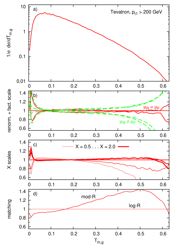
Fig. 1a illustrates the NLL+NLO matched distribution obtained in the log-R matching scheme with . The renormalisation and factorisation scales are chosen, event-by-event, to be in both the resummation and the NLO calculation. The distribution has a peak at small event-shape values that is characteristic of all resummed (and physical) event-shape distributions.
The uncertainty on the prediction is almost as important as the result itself, especially as it will allow us to gauge the significance of any disagreements that we will see with other predictive methods.
The most widely used form of uncertainty estimate is the variation of renormalization and factorization scales. The solid (red) curves in fig. 1b illustrate the effect of varying these scales simultaneously, showing the ratio of results with and to the default result. Except at very small event-shape values or at very large ones, where the distribution vanishes, one sees that the impact of symmetric scale variation is only about . Asymmetric scale variations are shown by the dashed (green) curves, corresponding to while keeping , and while keeping . For moderate and large values of the event shape they have a significantly larger impact than symmetric scale variations, of the order of for moderate . This highlights the importance of considering both symmetric and asymmetric variations.
Fig. 1c shows the impact of varying in eq. (3.24), with the line thickness increasing from to . As discussed in Sec. 3.2, this variation can be used to estimate the effect of higher order logarithms not included in our NLL resummation. We find that for moderate and large values of the effect is similar in size to the asymmetric renormalization/factorization scale variation. Closer to the peak of the distribution (where the bulk of events sits), the impact of the -scale variation is mildly larger. We also note that the variation is quite asymmetric: smaller values distort the central distribution much more than larger values.
Finally, in Fig. 1d we estimate uncertainties that arise from the details of the matching procedure. In particular we show the ratio of the mod-R matched distribution to the log-R (see eqs. (3.26), (3.27) and (3.28)). It is clear that at large values of , the difference between the two matched distributions is large, with differences of up to 45% for . These very large discrepancies occur however only in the tail of the distribution, where few events are present. Comparison to NLO at high (not shown) indicates that of the two matching schemes, log-R matching is the one with smaller higher order terms (i.e. its NLO+NLL result is closer to NLO) at large . In the following we will therefore use log-R matching as our default.
The above findings are representative of the results for the other event shapes considered here, both at the Tevatron and at the LHC and for the low- and high- samples (further NLO+NLL results are shown in Sec. 4.4 and on the website associated with this article [41]). In particular symmetric renormalization and factorization scale variation (as is currently done in many phenomenological studies) systematically underestimates the true size of theoretical uncertainties. While detailed error-estimate studies such as variation of X-scale and matching procedure are possible only for specific (resummed) calculations, an asymmetric and variation can be carried out for generic observables. This is perhaps most relevant for multi-scale observables, where the scale of is a priori not clear.
4.3 Comparison of resummed, NLO and matched results
In this section we compare various levels of fixed order calculations (LO, NLO), pure resummed ones (NLL) and matched ones (NLO+NLL) at the Tevatron for the high- sample. Because NLL+NLO resummations are rarely available (e.g. they are currently not available for non-global observables), we discuss in particular the extent to which NLO alone can be used to describe event shape distributions. As in the previous section we will use to illustrate our findings, but results are fairly independent of the specific event shape, the collider and the details of the hard cuts.
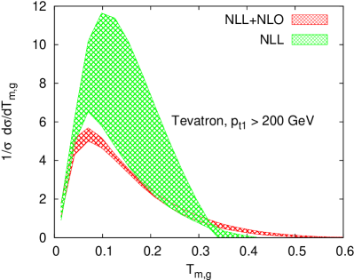
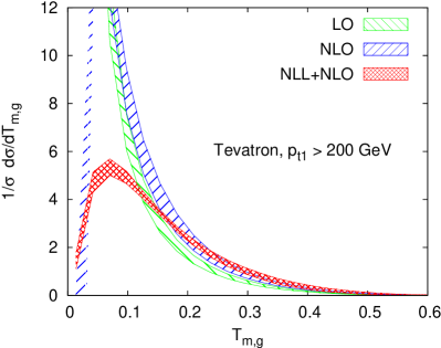
Fig. 2 shows the result for the log-R matched distribution compared to pure resummation (left) and pure NLO, and LO for reference (right). For the matched resummed result, the band corresponds to the span of all the uncertainties shown in fig. 1, while in the fixed order calculations it corresponds to the variations of just the renormalisation and factorisation scales (, with ); for the pure resummed result the band corresponds to the renormalisation, factorisation and -scale uncertainties.
As expected, the matched distribution agrees with the NLO results at large values of . However for the pure NLL resummation without any coefficient function obtained from eq. (3.23), the level of agreement with NLO+NLL is quite poor even at fairly small values of . For example, the position of the peak of the distribution is not all that well predicted (at rather than at ). As far as the height of the peak is concerned, both NLL and NLO+NLL distributions are normalized to one, however the NLL distribution becomes negative at , and this negative tail causes the distribution to be far too high at low . It is on the other hand reassuring that these large differences with the matched distribution are reflected in the very large uncertainty band of the NLL distribution.
As far as the fixed-order results are concerned, Fig. 2b, they are as expected divergent at small . The LO distribution essentially never agrees with the matched distribution, while the NLO does within uncertainties for . It is on the other hand evident that scale uncertainties of the NLO results at small underestimate the size of higher order corrections not included in the fixed order calculations.
Altogether, figure Fig. 2 highlights how neither NLO nor resummation alone can provide a sensible prediction, while the combination of NLO and resummation gives significantly reduced scale-dependence compared to either on its own. Furthermore the matching procedure gives the general shape that is associated with the resummation, while maintaining the large- behaviour of the NLO prediction. We finally note that for the event shapes presented here a LO+NLL resummation agrees well neither with the LO, nor with the NLO+NLL matched result.
4.4 NLL+NLO matched results for a range of observables
In the previous section we established that contrary to NLO or NLL alone, NLO+NLL provides robust theoretical predictions for event shapes distributions over a large range of the event-shape values. This section contains the bulk of results of the present work: we discuss NLL+NLO resummed distributions for a number of event shapes variables, both at the Tevatron and at the LHC and for both, low- and high- samples.
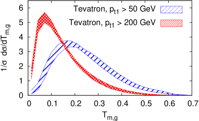
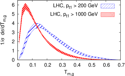
We start by looking at the effect of changing the hard selection cuts and the collider (Tevatron vs LHC) for the same observable discussed previously, , Fig. 3. There is a striking similarity between the Tevatron (left) and the LHC plot (right), both for the low- (Tevatron, GeV and LHC, GeV) and for the high- (Tevatron, GeV and LHC, GeV) samples. We also notice that low- curves are broader and peaked at a higher value of . This is a consequence of the higher prevalence of gluons in both the initial and final states of the hard scattering.
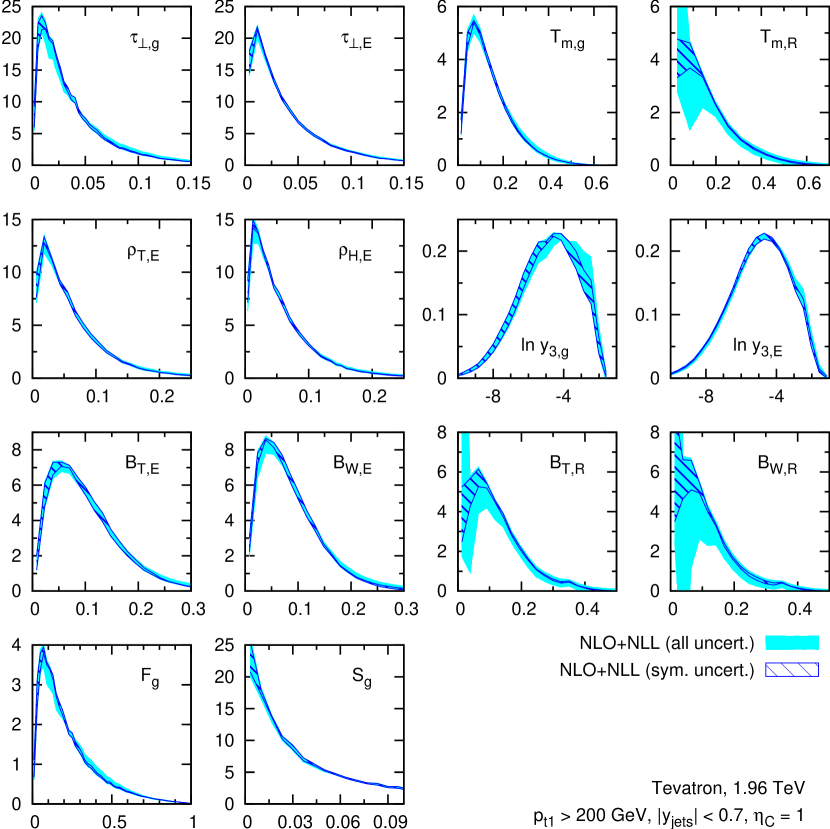
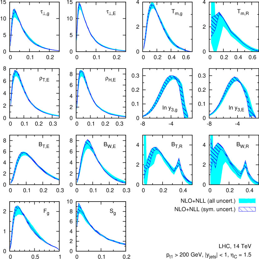
Because of this similarly between low- and high- samples at the two colliders, we examine results for a large range of observables, as defined in Sec. 2, just for the high- cuts at the Tevatron, Fig. 4, and for the low- cuts at the LHC, Fig. 5. For each observable, we give two uncertainty bands, one corresponding to a symmetric scale variation (hatched, dark blue) and one defined in terms of all theoretical uncertainties as discussed in Sec. 4.2 (solid, light blue). Comparing Fig. 4 and Fig. 5 we see that, as observed earlier for , the peaks of the distributions are further to the right and the distributions are broader for the LHC (low ) than for the Tevatron (high ). Looking at specific observables we see that, as already remarked in the case of for all observables the symmetric scale variation uncertainties are considerably smaller than the full uncertainties, and we stress that only the latter are really indicative of the size of all kinds of neglected higher order terms.
Some final remarks concerns the NLO+NLL results for , and . As discussed in [23] and at the end of Sec. 3.1.2, recoil variables are more difficult to resum than other variables, because in the caesar approach, the NLL term has an unphysical divergence at small values of the observable. This difficulty is reflected in the substantially larger uncertainty bands for these observables than for the directly global variants and those with an exponentially-suppressed forward term. Among the recoil variables, the thrust minor and broadenings were the only ones for which an even partially acceptable result could be obtained. In order to obtain results for recoil variables of similar quality to those for the other observables requires a resummation of initial state emissions in appropriate Fourier transform variables, as done e.g. for the Drell-Yan resummation [75], mixed with a Sudakov type resummation, as was done for the DIS broadening [76]. This is beyond the scope of caesar. Another characteristic to be commented on is the spike for and near . We believe this could be related to a Sudakov shoulder [77] type phenomenon, and similar (though less pronounced) artifacts have also been observed in DIS event-shape distributions. Again, it is beyond the scope of caesar to resum the enhanced higher-order terms associated with these structures.
4.5 Naive exponentiation of NLO
In the previous Section we presented full NLO+NLL resummations for a range of event shapes. Both the NLO Monte Carlo calculation and the NLL resummation are highly CPU intensive and are usually both run across many CPUs. While the NLO part of the calculation is the most computer intensive, this is to some degree counterbalanced by the fact that many observables can be computed in the same NLO run. The NLL resummation on the other hand requires essentially a separate run with caesar for each observable. Altogether, a single combination of collider energy and event-selection cuts requires many CPU-years of computing time. NLO+NLL resummation also requires that the NLO total cross section and LO distributions be decomposed into flavour channels, and this information is not available in the public version of nlojet++ (nor in most other public NLO codes). Furthermore, caesar is currently not public, the range of observables that can be resummed with caesar is not as broad as one might like (see Sec. 3.1.1), and the matching procedure at hadron colliders is not as straightforward as in , as discussed in Sec. 3.2. For the above reasons, it is interesting to explore the possibility of obtaining predictions with accuracy close to NLO+NLL using publicly available NLO results only. For instance the following combination of LO and NLO integrated, flavour summed distributions, and , and the corresponding total cross sections, and , as obtained directly from nlojet++,
| (4.1) |
has the following properties:
-
•
goes to 1 at , without corrections;
-
•
the fixed order expansion of the corresponding differential distribution, up to relative order reproduces the normalized NLO differential distribution;
-
•
the formal accuracy is not even LLΣ: starting from order the terms are only correct in the limit in which the event sample is dominated by a single colour channel.
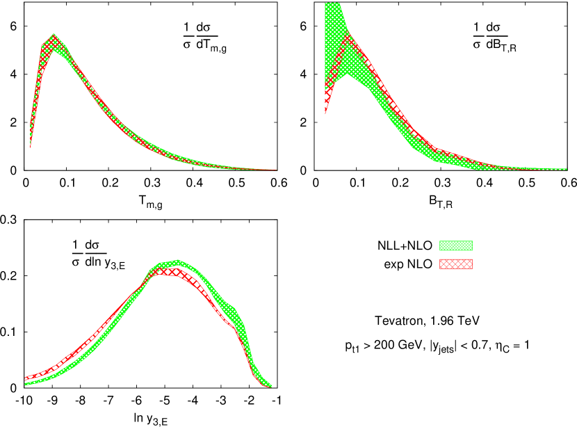
Though the method does guarantee any formal resummation accuracy, it is still instructive to see how it fares in practice. We therefore show in fig. 6 a comparison of NLO+NLL matched results with full uncertainties and the naive exponentiation of NLO, as defined in eq. (4.1) with full scale uncertainties for a representative set of observables for the Tevatron with a 200-GeV jet cut (similar results hold also at the LHC and for other cuts as well as other observables [41]). We see that for the directly global thrust minor (top, left) the exponentiation result is well-contained in the uncertainty band of the NLO+NLL matched result, suggesting that the naive exponentiation of NLO is indeed a quite reasonable procedure (similar results hold in general for global observables). The same observation is true also for the total broadening with recoil term (top, right) but with one important difference. In this case the NLO+NLL uncertainty band at small values of the observable is divergent, signaling the breakdown of the resummation (as discussed in [23] and at the end of Sec. 3.1.2). The scale uncertainty band of the naive exponentiation does of course not account for this and is small for all values of the observable. Therefore for observables like the recoil event shapes, whose double logarithms do not fully exponentiate, the naive exponentiation of the NLO results can only be used as long as one is far from the divergence of the pure NLL resummation (whose position is one of the pieces of information provided by caesar).
Finally, we show in fig. 6 (bottom, left) how well the naive exponentiation does in the case of the three-jet resolution parameter with exponentially suppressed term. We see that in this case the naive exponentiation result is not contained in the full uncertainty band of the NLO+NLL resummation. This is true for the tail of the distribution, where there seems to be too little radiation suppression and, similarly, for the peak, whose position is slightly displaced to the left. This softer spectrum is a feature of other exponentially suppressed observables as well (though the effect is not as remarkable).
Altogether it seems that naive exponentiation is a sensible procedure to extend the range of validity of pure NLO predictions. However, since it is not guaranteed to provide any formal logarithmic accuracy, one should rely on full NLO+NLL predictions for precision studies. In any case, we stress that before carrying out this exponentiation procedure, one should understand the basic soft/collinear properties of the observable (be it with caesar or in whatever other way).
4.6 Comparison with (matched) parton showers
For most practical applications, it is far more convenient to use parton-shower Monte Carlo event generators, like Herwig [3] or Pythia [4], or event generators merged with LO matrix elements, rather than a full NLL+NLO calculation. It can however be difficult to estimate the accuracy of these tools and the reliability of the error estimates that come with them. The purpose of this section is therefore to compare the NLL+NLO results with parton-shower based predictions (at parton level, in order to avoid non-perturbative corrections from hadronisation and the underlying event).
We will start with Herwig (v6.5) events showered from exact tree-level matrix elements for , and partonic scatterings, as generated with Alpgen [78]. We use the MLM prescription [79] to avoid double counting between emissions generated in the hard scattering and those generated by the parton shower. This combination of parton-shower and tree-level matrix elements is the standard tool for many Tevatron and LHC predictions.
To gauge uncertainties in the resulting matched samples we shall simultaneously vary the renormalisation and factorisation scales in the tree-level matrix elements by a factor of two around their default settings in the MLM procedure (which are taken as in the CKKW procedure [80]). The MLM procedure also involves a separation scale between the region of phase-space to be accounted for by the tree-level matrix elements or by the parton shower. We take this separation scale to be when we look at event samples whose hardest jet has and the angular distance for a jet and a parton to be matched is restricted to be . The hard events have been generated with a threshold for all partons (constrained to have ), which must separated from each other by a distance . In principle the MLM separation scale should also be varied in order to gauge uncertainties. However, the generation threshold should also be kept lower than the separation scale and the production of the tree-level event samples with the threshold already turned out to have very low efficiency and would have become prohibitive with much lower a threshold. Therefore we will only show results with a fixed separation scale. The PDF that we used was CTEQ5L [81], the default choice in Alpgen, but we also verified that the effect of switching to CTEQ6M (as used in our NLO+NLL calculations) was small.
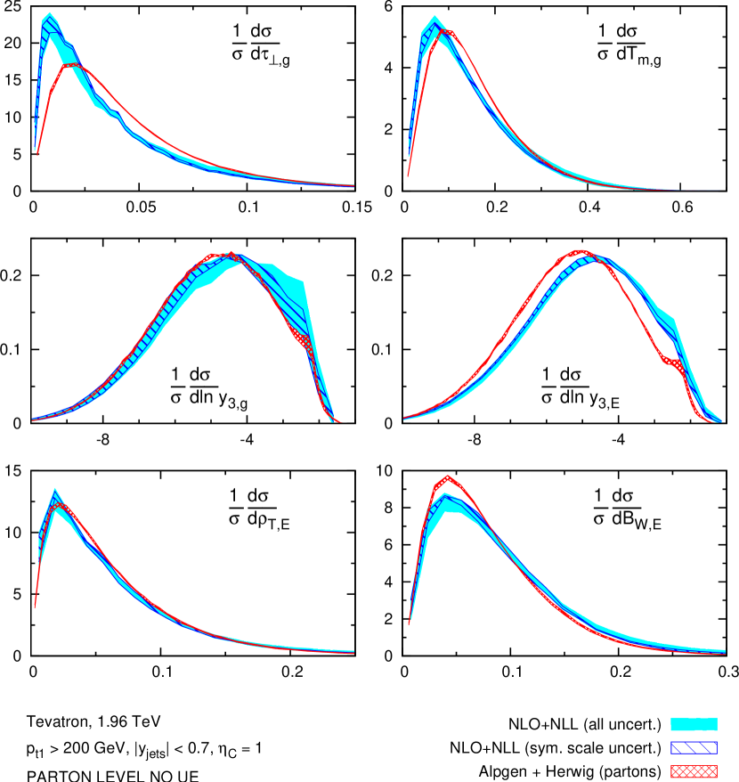
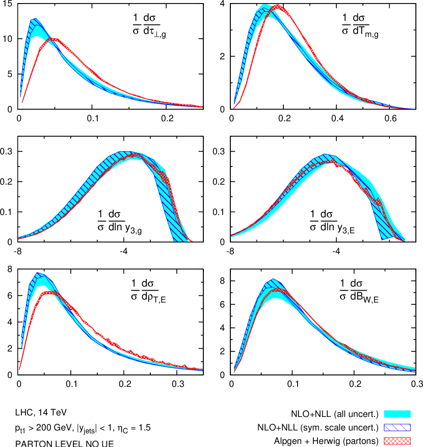
A comparison of the parton-level Alpgen+Herwig (Tree+PS) results with the NLL+NLO results is given in figs. 7 and 8, for collisions at Tevatron and LHC, with a cut of on the transverse momentum of the hardest jet. The Alpgen+Herwig results are shown as red cross-hatched bands. The NLO+NLL results are shown as two bands: a blue hatched band whose width corresponds to the uncertainty from just the symmetric variation of renormalisation and factorisation scales; and a cyan, solid band corresponding to the full set of uncertainties represented in fig. 1.
Generally, there is reasonable agreement between the Tree+PS and the NLO+NLL results. One feature of note is that the Tree+PS uncertainty band is significantly narrow than the NLO+NLL band (even that with just symmetric scale variation). It is not immediately obvious that this truly reflects smaller uncertainties in the Tree+PS case, which, based as it is on LO calculations, would be expected to show larger uncertainties than the NLO+NLL prediction. We tend instead to interpret this as indicating that symmetric scale variation does not provide a good estimate of the true uncertainty on Tree+PS predictions.131313It should be said that the uncertainty band on the Tree+PS prediction is considerably larger if one considers differential cross sections instead of normalised differential distributions.
There does not seem to be a clear pattern to the cases where there are significant differences between the two kinds of predictions. For example, for the and the variables the Tree+PS predictions seem harder than the NLL+NLO results. Instead, for , the Tree+PS results are generally softer.
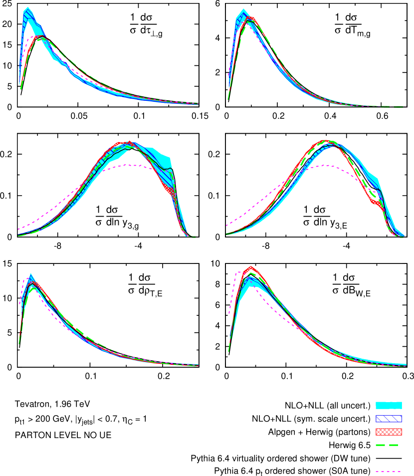
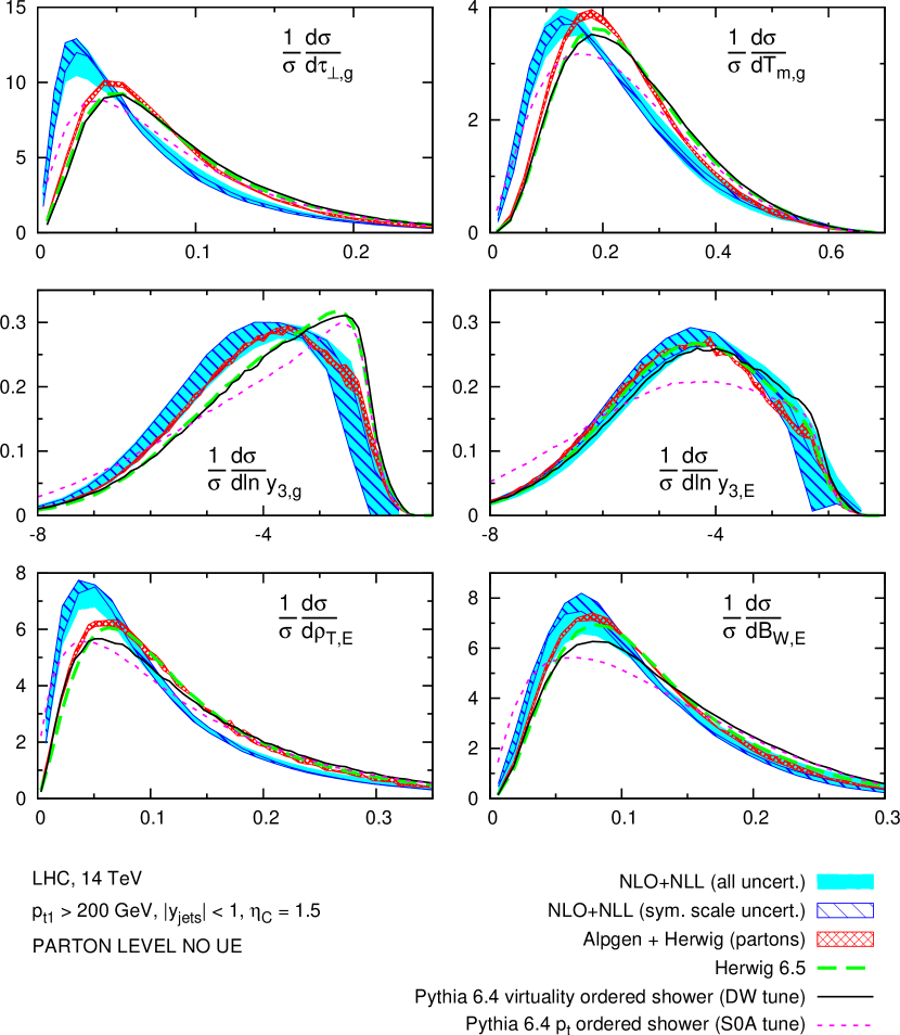
We also show in figs. 9 and 10 a comparison between results obtained from different shower Monte Carlo event generators with and without matching, for the same subset of the observables at the Tevatron and the LHC with a minimum on the hardest jet of . Pythia 6.4 is shown both for the old (virtuality ordered) and new (transverse-momentum ordered) showers. All results are shown at parton-level, without multiple interactions (i.e. no underlying event). For reference we show also the result of NLO+NLL resummation with symmetric scale variation uncertainties (the use of the full band would complicate the plots excessively).
In general Herwig’s angular-ordered shower and Pythia’s virtuality ordered (old) shower give results that are quite similar (or slightly harder) to the full matched results, with deviations visible in some cases, e.g. for at the LHC.
It is perhaps surprising that unmatched, plain parton shower results, are often harder and sometimes even closer to the NLL+NLO band than the Tree+PS matched ones, this is particularly evident for at the LHC. This is an unexpected result as the motivation for carrying out Tree+PS merging is that parton showers are unable to reproduce the structure of hard large-angle emissions.
What is also evident from figs. 9 and 10 is that there are big discrepancies between the newer, transverse-momentum ordered shower in Pythia 6.4 (in the S0A tune) and, essentially, everything else. These distributions appear to be significantly softer than those from other parton showers, with the difference most visible in the case of the variables, and inconsistent with the NLL+NLO calculation.
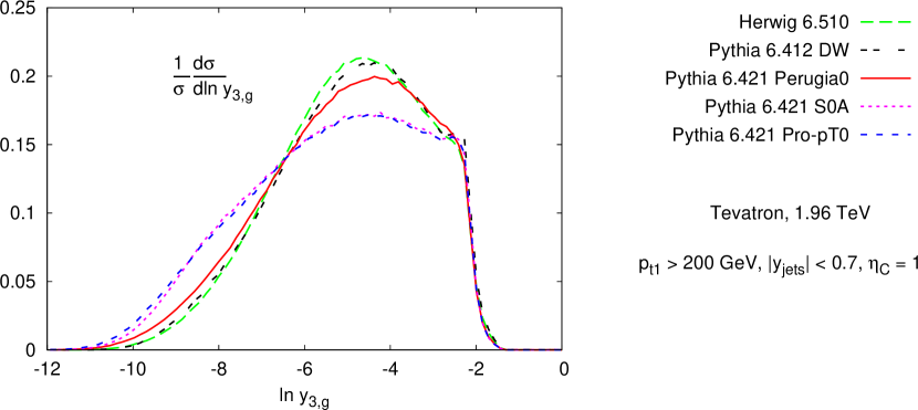
It is therefore useful to try to understand whether the origin of the discrepancies lies in the new shower or in the tuning of the Pythia parameters. To further probe this issue, we show in Figure 11 a comparison among plain Herwig, virtuality ordered (DW) Pythia and different tunings of the new transverse-momentum ordered shower, S0A [82], as used above, and two more recent tunes, Perugia0 [83] Pro-pt0 [84], (shown with version 6.421; version 6.412 yields identical results). Of these the two more recent -ordered tunes, Pro-pt0 gives results very similar to S0A, while Perugia0 is closer (though not identical) to the Herwig and virtuality-ordered Pythia results. The conclusion to be drawn from these results is that for transverse-momentum ordered showers, the shower parameters can have major implications for the reliability of the results and a consensus has yet to emerge among current tunes for the choices of these parameters.
5 Non-perturbative effects
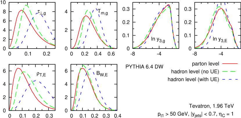
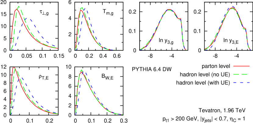
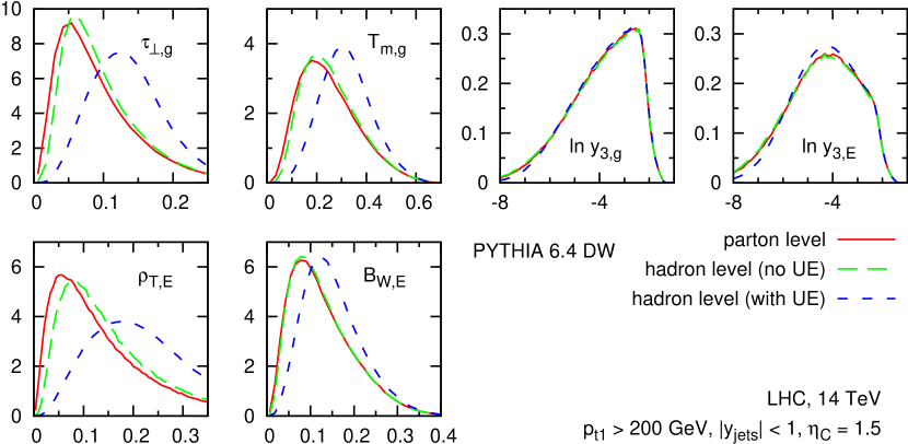
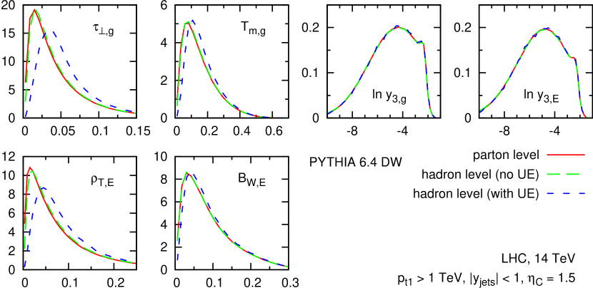
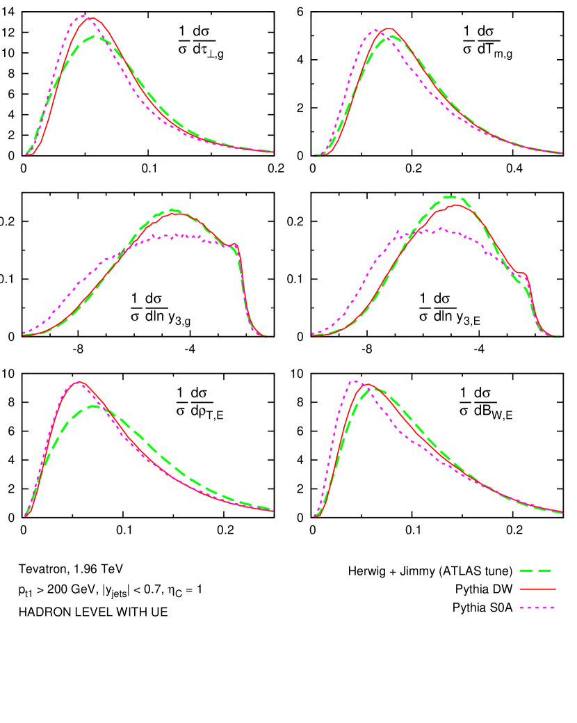
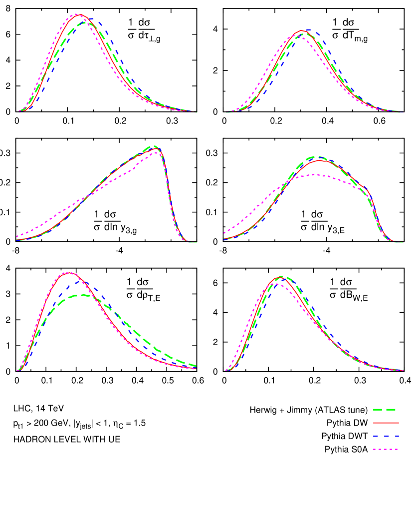
So far we discussed only perturbative effects, however, before any comparison to data can be done, non-perturbative effects have to be included. As in annihilation, there are non-perturbative effects due to hadronisation, i.e. related to the transition of partons to hadrons. In hadron-hadron collisions there are also interactions between the two beam-remnants, the so-called underlying event (UE). Both effects are suppressed by inverse powers of the hard scale of the high- scattering. For event shapes the dependence is linear in [85], while for jet-resolution parameters the dependence is even more suppressed, as will become evident also from the plots presented in this section.141414 A further potential non-perturbative effect is that due to in-time pileup, the additional (usually) soft collisions that take place during the same beam crossing as the hard collision of interest. Its impact can largely be eliminated by considering only events with a single primary interaction in the beam crossing. Given the huge cross-sections for the event selections outlined in table 2, this should not pose too much of a problem except, possibly, at the higher LHC cut.
At hadron colliders, analytical predictions for non-perturbative (NP) effects are available only for a limited number of jet-observbales [85, 86, 87, 88]. A more general way to estimate those effects is to use event generators, such as Herwig [3]or Pythia [4], which can be run at parton- or hadron-level with or without underlying event. The default Pythia underlying event model includes multi-parton interactions, while Herwig needs to be interfaced to Jimmy [89] to have a realistic modelling of the underlying event.
In Figs. 12-15, we compare parton level and hadron level results without and with UE for the set of observables discussed previously for the low- and high- samples at the Tevatron and at the LHC, as obtained with virtuality ordered Pythia 6.4 (DW tune).
As far as hadronisation corrections are concerned, one notices immediately that for event shapes these effects are quite large at the Tevatron for the GeV sample. They systematically shift the distributions to the right and distort them (mostly squeeze them). As expected these effects decrease considerably at GeV. Going from the Tevatron to the LHC, keeping the GeV cut, hadronisation correction are comparable, while again they decrease when going to the GeV sample, where they are completely negligible. Since the majority of events in a sample will have jets with close to the -cut, this patten confirms the expected scaling of hadronisation corrections. For distributions hadronisation effects follow the same pattern but are much smaller, and are already very small at the Tevatron for GeV.
The effect of the underlying event on these distributions is quite different. For event shape distributions at the Tevatron for , the UE broadens significantly the distributions and moves them systematically to the right. For fixed center of mass (c.o.m.) energy, the UE decreases with , but contrary to the hadronisation corrections, increasing the c.o.m. energy, at fixed results in an increased UE activity. As for hadronisation corrections, UE effects are much smaller for distributions than for event shapes. This fact means that at sufficiently high one can compare perturbative predictions directly to data, without additional NP corrections. This also makes distributions (in particular the global version) suitable for direct tuning of shower parameters. We note also that different event shapes have different NP sensitivities, broadenings seem to have smaller corrections, while masses and thrust distributions tend to have larger ones. Therefore the latter seem better suited to study NP effects and to tune models of hadronisation and underlying event.
To address this last issue further, we show in Fig. 16 how different Monte Carlo showers and tunes to the same Tevatron data differ from each other for the same set of observables. Specifically we use Herwig+Jimmy 151515 The parameters used are PRSOF=0, PTJIM, an inverse (anti)proton radius of JMRAD(73)JMRAD(91) and CTEQ6L1 [68] PDFs, as per the ATLAS tune in [90]. Pythia’s virtuality ordered shower with the DW tune and Pythia with the -ordered shower (S0A tune). It is noticeable how the DW, S0A and Herwig+Jimmy tunes differ (sometimes substantially), despite the fact that all have been tuned to Tevatron data. For S0A in particular this is not really surprising: if perturbative predictions already differ substantially, so will full results at hadron level. However it is nevertheless instructive, because it illustrates to what extent hadron-level event-shape distributions can help constrain perturbative aspects of the shower.
Finally, in Fig. 17 we show what happens for the same cut at the LHC. Discrepancies between Herwig and Pythia survive (but are maybe reduced). In addition to the DW Pythia tune, we also show DWT (which was identical at Tevatron energies) and see sizable differences between them. All this suggests that event shapes have significant scope for tunes of event generators.
6 Multi-jet limit
One common use of event shapes is to distinguish two different classes of multi-jet events: those in which the jets cover phase space quite uniformly, as in multi-body heavy-particle decays; and those in which the jets are relatively collimated in few bunches, as induced by the collinear singularities of massless QCD multi-particle emission. For example, the ATLAS [51] and CMS [52] discussions of prospective analyses mention the use of event shapes, most notably the transverse sphericity (see below), in physics studies that range from analyses to searches for supersymmetric particle decays and black-hole decays (yet other applications include hidden-valley searches [91, 92]).
The purpose of this section is to compare various event shapes’ ability to distinguish characteristically different event topologies. Firstly we shall examine to what extent current event shapes are able to distinguish symmetric 3-jet topologies from symmetric multijet topologies. The main finding will be that they discriminate principally between 2-jet pencil-like events and symmetric events, regardless of the number of jets in the latter. We shall then study the robustness of the identification of symmetric events: both with respect to parton showering and to the orientation of the multijet system. The results from these two studies will then lead us to propose event shapes that should have enhanced sensitivity to the symmetric multijet limit.161616 It is worth noting also the event-shape type observable proposed for BSM searches [93], whose aim is not to distinguish multijet “hedgehog” topologies from dijet topologies, but rather to be sensitive to the hadronic structure of BSM signal events with large transverse missing energy (e.g. -parity conserving SUSY), but without making explicit use of the measurement of missing transverse energy.
6.1 The transverse sphericity
One event shape that we have not considered so far is the sphericity. Since it is by far the most widely used for discriminating symmetric multi-jet topologies, let us briefly examine its properties. It is defined in terms of the eigenvalues of the transverse-momentum tensor:
| (6.1) |
It has the property that it tends to for events with circular symmetry in the transverse plane, and is for pencil-like events. However the appearance of a sum of squared momentum components in makes this observable collinear unsafe, as is the case [44] for the related variable in : for example, if a hard momentum along the direction is split into two equal collinear momenta, then their combined contribution to will be half that of the original momentum. Therefore collinear splittings change the sphericity by a factor of order 1. One consequence of this is that it is impossible to make perturbative predictions for the sphericity beyond leading order. Another consequence is that parton showering and hadronisation significantly alter the value of the observable, limiting its ability to discriminate different topologies (at least when the input momenta are particles; often it is jets that are used as inputs). We shall see this explicitly in section 6.3.
6.2 The circular limit
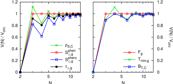
The simplest instructive study that comes to mind for event shapes intended to distinguish symmetrical multi-jet events from dijet events is to examine their values for perfectly symmetrical planar transverse events with varying numbers of momenta, for . This is illustrated in fig. 18. For uniformity the results have been normalised to the value obtained for perfectly circular planar events (), as given in table 3.
The only two observables with a monotonic (and trivial) behaviour are and . The remaining ones have been grouped into the left and right hand plots according to whether they peak for (thrust-like) or (broadening-like) and one sees that the perfectly circular limit does not give the largest value for all observables. Perhaps the most interesting observation from these plots is the modest difference between the -particle and fully circular events — thus they are sensitive to the absence of a unique preferred transverse direction, but not to the overall degree of symmetry of the event.
| 1 | 1 | 1 |
|---|
6.3 Collinear safety and showered events
Let us now ask the question of how much the collinear unsafety of matters in practice. To investigate this we have taken a number of partonic events and showered them with Herwig, using the “inclusive” MLM prescription [78] to reject events in which the showering introduces a fourth, harder jet, or other strong modifications of the event. Figure 19 shows the distribution of , and for two kinds of input partonic event, which are both planar with all particles at rapidity :
| Event 1 (generic) | Event 2 (Mercedes) | ||
|---|---|---|---|
| GeV, | GeV, | ||
| GeV, | GeV, | ||
| GeV, | GeV, | ||

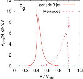
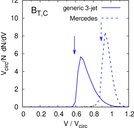
One clearly sees that the collinear unsafe has much less discriminating power between the two events than do or (or for that matter any of the other event shapes that were shown in fig. 18). Furthermore it is clear for the Mercedes event that the peak at has little connection with the expected 3-parton Mercedes value of . In contrast, the distributions for the other two observables are peaked close to the expected values (indicated by the arrows). This should of course be of no surprise given the collinear unsafety of . However, in view of the latter’s widespread current use (albeit with jets, rather than particles, as inputs), we feel that the point is worth noting.
6.4 Impact of event orientation
One of the interests of event-shape studies is in identifying massive particle decays. Most of the event shapes above have the counterproductive characteristic that they give very different results for particles that decay with just transverse components (in the particle’s centre of mass) or with both longitudinal and transverse components. To illustrate this, we take the generic event given above and rotate it by around the axis of particle , giving GeV, and rapidities . We shower it, as explained above, and the resulting distributions for three event shapes (normalised to their values in the circular limit) are shown in fig. 20.

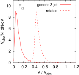
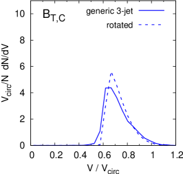
For and there is a large difference between the distributions for the generic and rotated-generic events (and similarly for e.g. , and ). For the broadening in contrast, which we recall involves both the and dispersions of particles with respect to axes in each of the two central half-regions, the generic and rotated-generic events give rather similar distributions. A similar phenomenon occurs with the invariant masses of those regions, in that masses too are sensitive to both directions of dispersion, though their intrinsic rotational invariance is in part spoiled when one normalises to as in eq. (2.17). The rotational invariance is probably in part the origin of the usefulness of “cluster-masses” in the context of hidden-valley studies [92]. Note however that masses are significantly more sensitive to (initial-state) forward semi-hard radiation than are broadenings.
6.5 Increasing sensitivity to the spherical limit
As is clear from figure 18, none of the event shapes above are particularly effective at distinguishing truly spherical events from simpler multi-jet topologies, like symmetric transverse-planar events.
What one has in mind when discussing spherical events is that they have significant “volume”, symmetrically distributed around the event. One way of obtaining sensitivity to this is to consider the following matrix, separately for the up and down central regions of an event:
| (6.2) |
where and , and similarly for the central down region, . The eigenvalues of have the property that is non-zero if there are two non-collinear particles in the hemisphere, while is non-zero if there are three non-coplanar particles in the hemisphere. The observable
| (6.3) |
which we name “supersphero”, is therefore non-zero only if there are 3 non-coplanar particles in each of the hemispheres of the event — i.e. for events that truly bear some resemblance to spherical events.
For a perfectly spherical event the two eigenvalues in each hemisphere are and .171717 One may balance the two eigenvalues more closely for example by replacing (i.e. with the first two terms of the expansion of ) in eq. (6.2), though there is a significant degree of arbitrariness in this choice.
The observable, in terms of its use of eigenvalues of a matrix, relates of course to the -parameter of eq. (2.4) and to the event shapes studied for boosted top-quark identification [26, 28]. The latter’s use of a matrix defined in the plane transverse to a jet is actually quite similar to our use of a matrix defined in a central half-region.
A detailed study of the observable would benefit from comparisons of high jet-multiplicity QCD samples and multijet samples from new-physics scenarios. Such a study is beyond the scope of this paper, but would, we believe, be of interest.
7 Summary of main results
Given the length of the paper, and the fact that we have addressed quite a range of issues, we find it useful, before concluding, to summarise here the main results of the paper.
There are a number of reason why event shapes provide a powerful laboratory for studying of a range of aspects of strong-interaction physics at hadron colliders. From an experimental point of view, cross sections for the QCD (dijet) events on which one carries out event-shape studies are very large both at the Tevatron and at the LHC. This means that high-statistics event samples are already available at the Tevatron and can be expected early on at the LHC. Since event shapes are defined as dimensionless ratios of combinations of hadron-momenta, and since their differential distributions are also dimensionless, many experimental uncertainties are reduced. From a theoretical point of view, one of the attractive characteristics of event-shape studies is that different variables provide complementary sensitivities to a broad variety of features of hadronic events, such as the topology of the final state, the nature of initial and final-state jet-fragmentation, hadronisation, and the underlying event.
The above points motivated us to study many hadron-collider event shapes in a single context. We exploited the automated NLL resummation procedure implemented in caesar to obtain next-to-leading logarithmic resummed distributions matched to next-to-leading order exact predictions from nlojet++ for a large number of event shapes at the Tevatron and at the LHC.
The matching procedure is conceptually simple, but technically involved, as discussed in detail in Sec. 3.2. One issue is that the best logarithmic accuracy achievable once NLO and NLL predictions are available, namely in the expansion of the integrated distribution, NNLLΣ, can be obtained only if the NLO code provides full information about the flavour of all incoming and outgoing partons. This decomposition into flavour channels is not present in the publicly available version of nlojet++, so we used the extended version developed in [94] in order to extract this information. We also needed to use the flavour- jet-algorithm of ref. [54] to map the flavour of events into that of an underlying Born-like event. Additionally we needed the order-by-order expansion of PDF evolution, which was provided by hoppet [64]. The computing effort should also not be neglected: our directory of resummed results contains files, and we estimate that several tens of years of CPU time have gone into the NLO and NLL calculations used here. Part of this complexity stems from our choice to consider several different classes of uncertainties associated with uncalculated higher-order terms: those from separate variation of renormalisation and factorisation scales; redefinition of the argument of the logarithm being resummed (-scale); and two choices of schemes for combining (matching) the NLO and NLL results.
Among the questions we asked was whether this considerable complexity is needed. It turned out that the flavour decomposition had only a modest effect (cf. Appendix A). We also found that a simple exponentiation of the NLO result, as presented in Sec. 4.5, not even correct to LL or LLΣ accuracy, comes remarkably close to reproducing most of the NLO+NLL distributions (albeit not close enough that one would forgo NLO+NLL if it is available). One interpretation is that the large amount of radiation that comes from the 4 Born legs in a process causes event-shape distributions to be dominated by regions where the logarithm that is being resummed is not all that large. Note, however, that plain (unexponentiated) NLO predictions are very inadequate substitutes for the full NLL+NLO result and their uncertainty bands are misleadingly small.
We studied three generic classes of event shapes: the directly global ones, those with exponentially suppressed terms and those with a recoil term. The definition of the observables is recaleld in sections. 2.1, 2.2, and 2.3 respectively. While stable numerical results could be obtained for observables belonging to the first two classes, for the last of these it was sometimes impossible to obtain numerically sensible results. This is in part due to cancellations among contributions from multiple emissions in the recoil term, which cause the resummation provided by caesar to have a divergence at small , as explained in Sec. 3.1.2. It is also due to structures in the middle of the physical region, akin to Sudakov shoulders [77], which would require an additional resummation. Such shoulders are visible e.g. for the broadenings with recoil term in Figs. 4 and 5. These observables are also challenging experimentally because the measurement of the recoil term is affected by cancellations between large transverse momenta of the two hard jets.
A question mark that hangs over NLL resummations is that of coherence-violating logarithms (CVL, referred to as super-leading logarithms (SLLs) in the context of interjet energy flow) [39, 40], terms potentially starting at , related to a violation of coherence, whose validity was a crucial assumption in the resummations of [31]. There is a risk that this could therefore invalidate our claim of NLL accuracy for some observables. We investigated this point in Sec. 3.3, and found that the answer depends critically on the ordering parameter used in the calculation of the SLL terms. If, as in [39, 40], one makes the assumption that the ordering parameter is transverse momentum, then the claim of NLL accuracy breaks down for our “exponentially suppressed” class of observable (not for the others), while NNLLΣ remains valid for all observables. If one instead assumes virtuality ordering, then both NLL and NNLLΣ accuracies should be valid for all our observables. This highlights the importance of understanding the question of ordering for SLLs, which also affects the coefficient of the terms in [39, 40] and probably requires that one go beyond the eikonal approximation that was used there. Nevertheless, practically we tend to believe that SLLs will not seriously affect our results, one reason being that we still retain NNLLΣ accuracy.
Turning to our phenomenological results, a feature common to all observables is that the shape of the distributions is strongly influenced by the ratio of quarks to gluons among the incoming partons. This is because the double-logarithmic Sudakov exponent, responsible for the position and width of the peak of the distribution for each underlying subprocess, is determined by the total color charge of the hard emitting partons. Event samples dominated by gluon scattering (Tevatron with GeV, LHC with GeV) have broader distributions than those dominated by quark scattering (Tevatron with GeV, LHC with GeV). This is evident e.g. in Fig. 3 in the case of our representative observable and is discussed in Sec 4.3. We remark that dijet event-shapes at hadron colliders are the first case in which a change in a kinematical cut modifies the double logarithmic behaviour of the event-shape distributions. This would not be the case for event shapes in hadron-collider processes such as Drell-Yan production, or +jet or +jet.
In the absence of data on the event shapes discussed here, one of the interesting uses of our NLL+NLO results is to compare them to the results of two Monte Carlo parton shower programs, this is discussed in Sec. 4.6. We considered Pythia 6.4 and Herwig 6.5 both without and (in the case of Herwig) with matching to multi-parton tree-level matrix elements (Alpgen, MLM prescription). The quality of the agreement between plain parton showers and the resummations depends significantly on the quark/gluon admixture: in quark-dominated event samples it is often adequate, while in gluon-dominated samples it is somewhat poorer. This may be a reflection of the extensive tuning of quark parton showers carried out with LEP data, while gluon parton showers have seen fewer constraints. The importance of tuning parton showers in a context with incoming beams is highlighted particularly strongly by the results of the newer -ordered shower in Pythia 6.4. In two tunes, S0A and Pro-Pt0, the agreement both with NLO+NLL and with other showers is quite poor; in the Perugia0 tune it improves, as can be seen from Fig. 11.
One might expect that supplementing parton showers with matching to multi-parton tree-level events (Tree+PS) should improve the agreement with NLO+NLL results. This is the case only for some of the observables. We also examined the impact of (simultaneous) renormalisation and factorisation scale variation on the Tree+PS results and found that it leads to an uncertainty estimate that is far smaller than the actual differences between Tree+PS and NLO+NLL results, as can be seen in Figs. 7 and 8.181818More precisely: it was significant on the 2, 3 and 4-jet differential cross sections, but mostly cancelled in the normalised event-shape distributions. This should not be surprising: in the NLO+NLL calculations simultaneous scale variation represented only a small part of the full uncertainties. Questions that remain open therefore are whether in the Tree+PS approach uncertainties can be more faithfully estimated if one examines further “handles” (independent scale variation, matching scale, etc.), and whether we would have reached similar conclusions with other matching schemes (e.g. CKKW) and programs.
From a non-perturbative point of view, we estimated both hadronisation and UE corrections using Monte Carlo event generators, as discussed in Sec. 5. As expected, hadronisation corrections decrease when increasing the -cut on the jets. They are fairly negligible with cuts of the order of GeV both at the Tevatron and at the LHC, as can be seen in Figs. 13 and 14. For lower cuts, they shift the distributions to the right and, for some observables they squeeze them, see e.g. Figs. 12. For jet resolution parameters ( and ) hadronisation effects are always small, just a few percent correction for at the Tevatron, much smaller in all other cases. These observations are consistent with the experience obtained from and DIS event-shape studies.
As concerns the UE, there are observables for which it has a sizable effect even at , most notably for the thrusts and jet-masses, as can be seen in Fig. 15. This means that these event shapes are particularly good for tunes of the UE. Jet-resolution parameters are the only observables for which the UE effects remain consistently small (a few percent for the lower -cut samples, even smaller for the large ones). They are therefore well suited for tunes of perturbative parameters of showers and in general for perturbative studies.
Finally, in Sec. 6 we examined how well event shapes can discriminate QCD-like two-jet events from BSM-like multi-jet events, and how robust this discriminating power is with respect to parton shower (radiative) corrections. In general we find that event-shapes discriminate well between events with two or more than two jets, but they do not discriminate well between three or any large number of jets: the value of event-shapes does not even increase monotonically with the number of jets for symmetric events, see Fig. 18 in Sec. 6.2. On the other hand it is possible to design new event shapes, which start with six jets in the final state, as is the case for our “supersphero” event shape defined in Sec. 6.5. We believe these might be particularly promising for extracting new-physics signals that involve relatively isotropic events with high jet multiplicity. Other considerations that we examined in Sec. 6.3 include how well event shapes retain their discriminatory power after parton showering (the collinear-unsafe, but widely used transverse sphericity, whose definition is recalled in Sec. 6.1 is particularly poor in this respect); and also their sensitivity not just to transverse event structure, but also to longitudinal event structure (the broadenings do well at treating both on an equal footing).
8 Conclusions
In this article we have shown the first NLO+NLL (NNLLΣ) predictions, with full uncertainty bands, for hadronic observables at and colliders. We opted to make these predictions for event shapes in the context of dijet production, bringing together calculations with caesar and a specially adapted version of nlojet++, despite the fact that the NLO+NLL matching is technically more challenging than for event shapes in other hadron-collider processes such as Drell-Yan [24] or W/Z+jet [22] production.
Several properties of the dijet process motivated our choice: it involves both initial and final-state partons; it offers the freedom to vary the proportion of quarks and gluons involved in the Born process, through the cut on the hard jets; when that cut is placed at moderate , dijet production involves a substantial scattering component, offering the most accessible example of a gluon-dominated process; and the cross sections imply large event samples.
Comparisons of our results with parton-shower Monte Carlo predictions revealed adequate agreement for historic showers (Herwig 6.5, virtuality-ordered Pythia 6.4) in quark-dominated cases, while the showers were generally too hard in gluon-dominated processes. Some common tunes of the newer, -ordered shower in Pythia 6.4 fared noticeably worse than the historic showers. We also examined one framework for matching to multi-parton tree-level matrix elements (MLM matching of Alpgen+Herwig 6.5). Though it led to some improvements, it was not immediately sufficient to bring about systematic agreement with the NLO+NLL results. These findings illustrate how event shapes can provide substantial input to the quest of understanding perturbative QCD at hadron colliders.
At hadron level, some event shapes are subject to significant non-perturbative corrections from hadronisation and the underlying event. We saw this to be the case, for example, for the thrusts and jet masses, while other observables, notably the variants, were largely unaffected by non-perturbative effects. Studying a broad range of event shapes, as done here, therefore provides complementary information on QCD phenomena at hadron colliders at many different physical scales.
Event shapes are of interest not just for constraining QCD dynamics, but also for discriminating BSM-like multi-jet topologies from more QCD-like events. There are many interesting questions to ask about event shapes in this context. Some that we addressed here include their robustness to parton showering (the widely used transverse sphericity fares poorly), their sensitivity to longitudinal versus transverse event structure and their behaviour in the high jet multiplicity limit, where new dedicated event shapes, like the supersphero variable introduced here, can have particular advantages.
These first steps of ours in exploring the phenomenology of event shapes at hadron colliders open a window onto a broad range of possible new studies, both theoretical and experimental. We look forward to their future development.
9 Acknowledgments
We thank Mrinal Dasgupta, Günther Dissertori, Pino Marchesini, Lester Pinera, Peter Skands, Mike Seymour, Matt Strassler, Jesse Thaler and Matthias Weber for fruitful discussions on this subject. We thank CERN, Milano-Bicocca University, the LPTHE (UPMC Univ. Paris 6) and ETH Zürich for hospitality while part of this work was carried out. A.B. would like to thank Craig Prescott and the High Performance Computer center at the University of Florida for the use of computing facilities in an earlier stage of this work. G.Z. is supported by the British Science and Technology Facilities Council. The work of G.P.S. is supported in part by the Agence Nationale de la Recherche under contract ANR-09-BLAN-0060.
Appendix A Cross-checking fixed order and resummation
Part of the value of having separate resummed and fixed-order calculations for event-shape distributions is that they provide cross-checks as to the validity of each of the approaches. This check is usually performed by a comparison of the exact fixed order results in eq. (3.5) with the expansion of the resummed result from section 3.1. At small the two results should differ order-by-order only by terms suppressed by powers of or by logarithmically enhanced terms that are neglected within the resummation accuracy of .
At order , the distribution of eq. (3.2) has the expansion at small
| (A.1) |
where is the coefficient of , has the dimension of a cross section and implicitly contains (notice that is of order ). A NLL resummation predicts and , while is obtained from the coefficient of eq. (3.18) by summing over all subprocesses corresponding to the same colour channel , as indicated in eq. (A.1). The constant can be extracted from the exact fixed cross sections and , defined as in eq. (3.6), as follows:
| (A.2) |
Fig. 21a shows the prediction for the differential distribution obtained from eq. (A.1), compared to the exact result from nlojet++, for the total transverse thrust . The two distributions agree at small .
Since fig. 21a contains large logarithms, a better visual constraint can be obtained by plotting the difference between and its logarithmically-enhanced part , which should go to a constant at small , and indeed does. By performing this exercise separately for each colour channel one can obtain the individually, and can also verify that vanishes for small . From one can extract the colour-decomposed average coefficient constant .
The coefficients obtained in this way are not precisely the ones that multiply the resummed distribution according to either of the two matching procedures described in section 3.2, because there one resums not logarithms of but of a rescaled quantity , eq. (3.24). To get an idea of the size of the term as it is relevant in the matched resummations, instead of plotting , in fig. 21b we plot the difference between and the distribution
| (A.3) |
where is the constant of eq. (3.25) computed for the reference Born configuration used for the analysis of the event-shape properties in caesar (two hard jets in the centre-of-mass frame with an angle with respect to the beam corresponding to ). The constants and are defined in terms of the so as to give equality between the middle and right-hand sides of eq. (A.3). One observes that the difference in fig. 21b (normalised to ) goes, as expected, to a constant. That constant should be of order , whereas numerically it is . However, we also know from table 2 that the order corrections can come with large coefficients.
Given the and the corresponding NLL resummations , one can predict the NNLLΣ terms in the expansion of , i.e. terms with . Specifically, to second order in , we have
| (A.4) |
and to NNLLΣ accuracy we should control , and . To see that this is the case we compare to the resummation prediction for the modified integrated distribution
| (A.5) |
where again the constants and are defined so as to given agreement between the middle and right-hand sides of eq. (A.5). Fig. 21c shows the exact second-order differential distribution ,191919 As mentioned at the beginning of section 3, there is an unknown overall constant in , which relates to the NNLO coefficient of the dijet cross-section. This is irrelevant for us here, since we only use the derivative of . compared to obtained from eq. (A.5).
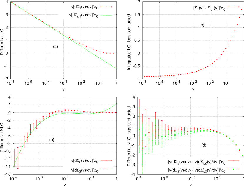
Again one sees good agreement, which is more readily verified by examining the difference between the two distributions, fig. 21d, which is supposed to be (and is) flat (the constant results from differentiation of the term in eq. (A.5)). We also include the result that is obtained (lower points with errorbars) if one does not carry out the colour decomposition for , but just computes . This gives rise to a different expansion, , whose coefficient of is different from that of . For one notices that the corresponding difference between the exact result and the distribution exhibits a hint of a slope at small , indicating a missing term in .
Fig. 22 shows the same comparison of fig. 21 for the global thrust-minor . In this case one is not able, within errorbars, to see any difference between a resummed prediction containing , giving the correct , and one based on , as is evident from Fig. 22d. This is possibly due to the fact that the difference between the full results and the first order expansion of the resummation, shown in Fig. 22a, is small.
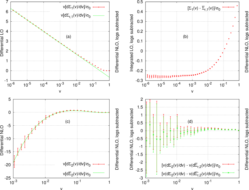
A.1 Weighted recombination in NLO calculations
NLO Monte Carlo calculations for multi-jet processes are highly CPU intensive. Consequently, one carries out multiple calculations (runs), spread across many CPUs, and averages them so as to get the final result. The correct way of determining the average is to weight each run in proportion to its number of events. In practice, however, it is common for the distribution of each run to contain one or two bins that are “outliers”, obviously inconsistent with the distribution as a whole, and which are a consequence of a handful of real and subtracted NLO events with very large opposite-sign weights that end up in different bins. These outliers lead to visible anomalies also in the number-weighted average and make it almost impossible to use the final distribution without some (often questionable) prescription to deal with the outlying bins.
A common alternative to number-weighted averaging is, for each bin of a run, to choose a weight that is inversely proportional to the square of the bin’s error in that run. This is an option for example in nlojet++ (and is implicit also for the total cross section in programs like MCFM [95] that use VEGAS). Since outlier bins tend to have much larger errors than normal bins, they contribute little to the average, resulting in much smoother final distributions. However, the error-weighted averaging procedure introduces a bias, because there tends to be a correlation between the value in a bin and its error: for example, in event samples with positive-definite weights, it is well known that runs with larger bin values also have larger errors, and the final error-weighted average systematically undershoots the correct result.
Fig. 23 shows the analogue of fig. 21, comparing event number-based and error-based weighting. At large negative values of there is a clear slope, i.e. the bias in the error-weighted procedure causes the result to disagree with the expectations based on resummation. Only with number-weighted averaging does one obtain results like fig. 21, which show agreement between the logarithmic structure of the NLO and resummed calculations.
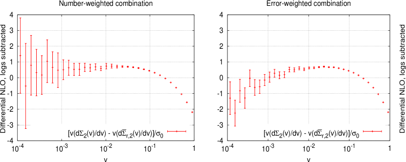
So as to deal systematically with the issue of outlying bins figs. 21 and 22 use a modified version of the number-based weighting, as follows. One first determines an error-based average for a bin , and a corresponding uncertainty on its contents — this provides an estimate for the correct value. One then carries out the number-based average with the following modification: for a given bin, one excludes runs whose result is further than from the (we use for 15 runs; should scale as the square-root of the number of runs). This then gives us a final result that is smooth and with a substantially reduced bias relative to an error-weighted recombination.
Note that in the phenomenological plots of sections 3 and 4 we have used the error-based recombination weights. On one hand the bias that it introduces is modest compared to uncertainties from subleading effects. On the other, some of our runs used Rambo [96] phase space and others the dipole [97] phase space, and this automatically privileges whichever of the two gives best convergence in a given phase-space region.
Appendix B Comment on effect of forward rapidity cut
For both generic global event shapes and those with an exponentially suppressed forward term, in order to satisfy the globalness requirement needed for the NLL resummation, we included all particles in the event, including those in the forward/backward regions. Experimentally however, it is not possible to perform measurements up to infinite rapidity. At the Tevatron the forward detector coverage goes up to and, at the LHC, measurements up to are viable. Theoretical arguments suggest that as long as the event-shape’s value is not too small, the effect of not including forward emissions should be negligible [22], specifically if , with given by [23]
| (B.1) |
where the and parameters were discussed in section 3.1.1. Examining the pure resummed distributions in [23], we came to the conclusion that the result in eq. (B.1) for ensured that the cutoff would usually have an impact only well below the maximum of the distributions. Here we supplement this analysis with a numerical study that investigates the impact of the rapidity cut in practice.
For this purpose we compute the NLO+NLL prediction using a rapidity cut on input particles for the NLO part of the calculation and compare this to the full NLO+NLL without forward rapidity cuts. In parallel we carry out an estimate using a Monte Carlo event generator, since it is straightforward to run it with a rapidity cut.
Fig. 24 shows comparisons between NLO+NLL with (solid line) and without the cut (full uncertainty band), as well as the corresponding Monte Carlo predictions obtained with Herwig (without UE) at parton level at the Tevatron ( GeV). Fig. 25 shows the corresponding results at LHC ( GeV). The results with the rapidity cut are always contained in the full uncertainty band of the results without. Furthermore, there is in general very little difference between the two Monte Carlo predictions, with the exception of the directly global transverse thrust, which is the observable most sensitive to forward emissions, as the weight of emissions in the forward region is large compared to that of emissions inside the jets. We note that this is also the one observable where the difference between Monte Carlo predictions and NLO+NLL is largest.
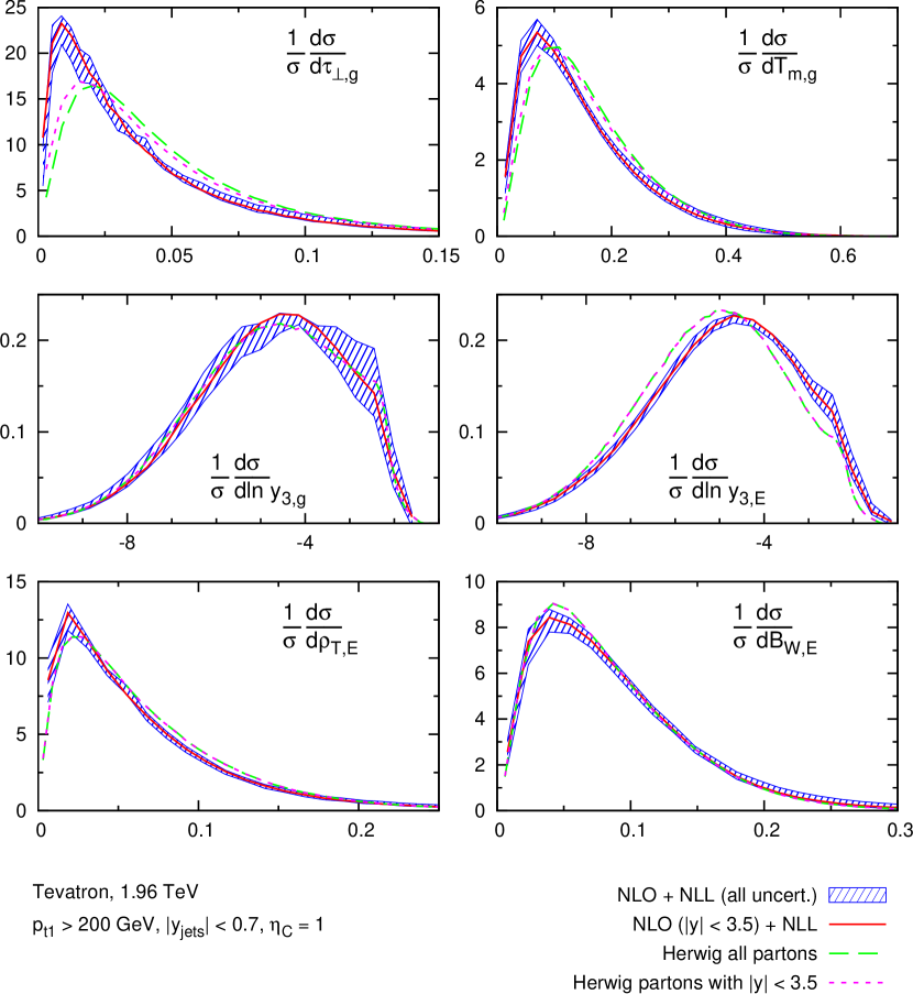
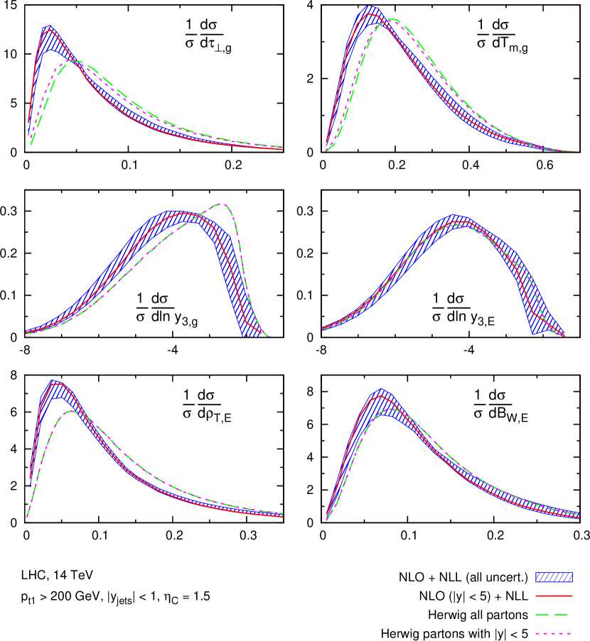
References
- [1] S. Kluth et al., Eur. Phys. J. C 21, 199 (2001) and references therein.
- [2] S. Bethke, Nucl. Phys. Proc. Suppl. 121 (2003) 74 [hep-ex/0211012].
- [3] G. Marchesini, B. R. Webber, G. Abbiendi, I. G. Knowles, M. H. Seymour and L. Stanco, Comput. Phys. Commun. 67 (1992) 465. G. Corcella et al., JHEP 0101 (2001) 010 [hep-ph/0011363].
- [4] T. Sjostrand, S. Mrenna and P. Skands, JHEP 0605 (2006) 026 [arXiv:hep-ph/0603175].
- [5] L. Lönnblad, Comput. Phys. Commun. 71 (1992) 15.
- [6] P. Abreu et al. (DELPHI Collaboration), Z. Phys. C73 (1996) 11.
- [7] G. P. Korchemsky and G. Sterman, Nucl. Phys. B 437 (1995) 415 [hep-ph/9411211]; Y. L. Dokshitzer and B. R. Webber, Phys. Lett. B 352 (1995) 451 [hep-ph/9504219]; M. Beneke and V. M. Braun, Nucl. Phys. B 454 (1995) 253 [hep-ph/9506452]; R. Akhoury and V. I. Zakharov, Nucl. Phys. B 465 (1996) 295 [hep-ph/9507253]. Yu. L. Dokshitzer, G. Marchesini and B. R. Webber, Nucl. Phys. B 469, 93 (1996) [hep-ph/9512336]; M. Dasgupta and B. R. Webber, Eur. Phys. J. C 1 (1998) 539 [hep-ph/9704297]; Y. L. Dokshitzer and B. R. Webber, Phys. Lett. B 404 (1997) 321 [hep-ph/9704298]. Y. L. Dokshitzer, A. Lucenti, G. Marchesini and G. P. Salam, JHEP 9805, 003 (1998) [hep-ph/9802381]; G. P. Korchemsky and G. Sterman, Nucl. Phys. B 555 (1999) 335 [hep-ph/9902341]; M. Dasgupta, L. Magnea and G. Smye, JHEP 9911 (1999) 025 [hep-ph/9911316]; E. Gardi and J. Rathsman, Nucl. Phys. B 638 (2002) 243 [arXiv:hep-ph/0201019]; C. Lee and G. Sterman, In the Proceedings of FRIF workshop on first principles non-perturbative QCD of hadron jets, LPTHE, Paris, France, 12-14 Jan 2006, pp A001 [arXiv:hep-ph/0603066].
- [8] M. Beneke, Phys. Rept. 317, 1 (1999). [hep-ph/9807443].
- [9] M. Dasgupta and G. P. Salam, J. Phys. G 30 (2004) R143 [hep-ph/0312283].
- [10] Y. L. Dokshitzer, A. Lucenti, G. Marchesini and G. P. Salam, JHEP 9801 (1998) 011 [arXiv:hep-ph/9801324].
- [11] M. Dasgupta and G. P. Salam, Phys. Lett. B 512, 323 (2001) [hep-ph/0104277]; JHEP 0203 (2002) 017 [hep-ph/0203009].
- [12] A. Banfi, G. P. Salam and G. Zanderighi, JHEP 0201 (2002) 018 [arXiv:hep-ph/0112156].
- [13] V. Antonelli, M. Dasgupta and G. P. Salam, JHEP 0002, 001 (2000) [arXiv:hep-ph/9912488].
- [14] A. Gehrmann-De Ridder, T. Gehrmann, E. W. N. Glover and G. Heinrich, JHEP 0712 (2007) 094 [arXiv:0711.4711 [hep-ph]].
- [15] T. Becher and M. D. Schwartz, JHEP 0807 (2008) 034 [arXiv:0803.0342 [hep-ph]].
- [16] S. Weinzierl, Phys. Rev. Lett. 101 (2008) 162001 [arXiv:0807.3241 [hep-ph]].
- [17] M. Dasgupta and G. P. Salam, J. Phys. G 30 (2004) R143 [arXiv:hep-ph/0312283].
- [18] F. Abe et al. [CDF Collaboration], Phys. Rev. D 44 (1991) 601.
- [19] I. A. Bertram [D0 Collaboration], Acta Phys. Polon. B 33, 3141 (2002).
- [20] Christina Mesropian, Talk given at the “XVII International Workshop on Deep-Inelastic Scattering and Related Subjects”, DIS 2009, 26-30 April 2009, Madrid, see http://indico.cern.ch/materialDisplay.py?contribId=286&sessionId=3&materialId=slides&confId=53294
-
[21]
Z. Nagy,
Phys. Rev. Lett. 88, 122003 (2002);
[hep-ph/0110315];
Z. Nagy, Phys. Rev. D 68 (2003) 094002 [arXiv:hep-ph/0307268]. - [22] A. Banfi, G. Marchesini, G. Smye and G. Zanderighi, JHEP 0108 (2001) 047 [hep-ph/0106278].
- [23] A. Banfi, G. P. Salam and G. Zanderighi, JHEP 0408 (2004) 062 [arXiv:hep-ph/0407287].
- [24] I. W. Stewart, F. J. Tackmann and W. J. Waalewijn, arXiv:0910.0467 [hep-ph].
- [25] G. Dissertori, F. Moortgat and M. A. Weber, arXiv:0810.3208 [hep-ph].
- [26] J. Thaler and L. T. Wang, JHEP 0807 (2008) 092 [arXiv:0806.0023 [hep-ph]].
- [27] L. G. Almeida, S. J. Lee, G. Perez, I. Sung and J. Virzi, Phys. Rev. D 79, 074012 (2009) [arXiv:0810.0934 [hep-ph]].
- [28] L. G. Almeida, S. J. Lee, G. Perez, G. Sterman, I. Sung and J. Virzi, Phys. Rev. D 79, 074017 (2009) [arXiv:0807.0234 [hep-ph]].
- [29] G. P. Salam, arXiv:0906.1833 [hep-ph].
- [30] N. Brown and W. J. Stirling, Phys. Lett. B 252 (1990) 657.
- [31] A. Banfi, G. P. Salam and G. Zanderighi, JHEP 0503 (2005) 073 [arXiv:hep-ph/0407286].
- [32] S. Catani, L. Trentadue, G. Turnock and B. R. Webber, Nucl. Phys. B 407 (1993) 3.
- [33] D. de Florian and M. Grazzini, Nucl. Phys. B 704 (2005) 387 [arXiv:hep-ph/0407241].
- [34] D. de Florian and M. Grazzini, Phys. Rev. Lett. 85 (2000) 4678 [arXiv:hep-ph/0008152].
- [35] G. Bozzi, S. Catani, D. de Florian and M. Grazzini, Phys. Lett. B 564 (2003) 65 [arXiv:hep-ph/0302104].
- [36] T. Gehrmann, G. Luisoni and H. Stenzel, Phys. Lett. B 664 (2008) 265 [arXiv:0803.0695 [hep-ph]].
- [37] A. Banfi, G. Marchesini and G. Smye, JHEP 0208 (2002) 006 [arXiv:hep-ph/0206076].
- [38] H. Weigert, Nucl. Phys. B 685 (2004) 321 [arXiv:hep-ph/0312050].
- [39] J. R. Forshaw, A. Kyrieleis and M. H. Seymour, JHEP 0608 (2006) 059 [arXiv:hep-ph/0604094].
- [40] J. R. Forshaw, A. Kyrieleis and M. H. Seymour, JHEP 0809 (2008) 128 [arXiv:0808.1269 [hep-ph]].
-
[41]
A. Banfi, G. P. Salam and G. Zanderighi,
http://www.lpthe.jussieu.fr/~salam/pp-event-shapes/ . - [42] M. Dasgupta and G. P. Salam, JHEP 0208 (2002) 032 [arXiv:hep-ph/0208073].
- [43] M. Weber, private communication.
- [44] E. Farhi, Phys. Rev. Lett. 39 (1977) 1587.
- [45] G. C. Fox and S. Wolfram, Phys. Rev. Lett. 41 (1978) 1581; ibid., Nucl. Phys. B 149 (1979) 413 [Erratum-ibid. B 157 (1979) 543].
- [46] A. Banfi, G. P. Salam, G. Zanderighi, unpublished 2004, at http://www.qcd-caesar.org/ and http://home.fnal.gov/~zanderi/Caesar/Observables/Obs_ee/node7.html.
- [47] S. Catani, Y. L. Dokshitzer, M. H. Seymour and B. R. Webber, “Longitudinally invariant K(t) clustering algorithms for hadron hadron collisions,” Nucl. Phys. B 406, 187 (1993).
- [48] S. D. Ellis and D. E. Soper, “Successive Combination Jet Algorithm For Hadron Collisions,” Phys. Rev. D 48, 3160 (1993) [hep-ph/9305266].
- [49] G. C. Blazey et al., hep-ex/0005012.
- [50] L. Clavelli, Phys. Lett. B 85 (1979) 111; T. Chandramohan and L. Clavelli, Nucl. Phys. B 184 (1981) 365; L. Clavelli and D. Wyler, Phys. Lett. B 103 (1981) 383.
- [51] G. Aad et al. [The ATLAS Collaboration], arXiv:0901.0512 [hep-ex].
- [52] G. L. Bayatian et al. [CMS Collaboration], J. Phys. G 34 (2007) 995.
- [53] M. Dasgupta and G. P. Salam, JHEP 0208, 032 (2002) [hep-ph/0208073].
- [54] A. Banfi, G. P. Salam and G. Zanderighi, Eur. Phys. J. C 47 (2006) 113 [arXiv:hep-ph/0601139].
- [55] J. C. Collins, D. E. Soper and G. Sterman, Nucl. Phys. B 250 (1985) 199.
- [56] J. Botts and G. Sterman, Nucl. Phys. B 325, 62 (1989).
- [57] N. Kidonakis and G. Sterman, Phys. Lett. B 387 (1996) 867; Nucl. Phys. B 505 (1997) 321 [hep-ph/9705234].
- [58] N. Kidonakis, G. Oderda and G. Sterman, Nucl. Phys. B 531, 365 (1998) [hep-ph/9803241].
- [59] G. Oderda, Phys. Rev. D 61 (2000) 014004 [hep-ph/9903240].
- [60] N. Kidonakis and J. F. Owens, Phys. Rev. D 63, 054019 (2001) [hep-ph/0007268].
- [61] J. Kodaira and L. Trentadue, Phys. Lett. B 112 (1982) 66; J. Kodaira and L. Trentadue, Phys. Lett. B 123 (1983) 335.
- [62] J. C. Collins and D. E. Soper, Nucl. Phys. B 193 (1981) 381 [Erratum-ibid. B 213 (1983) 545]; J. C. Collins and D. E. Soper, Nucl. Phys. B 197 (1982) 446.
- [63] Y. L. Dokshitzer, G. D. Leder, S. Moretti and B. R. Webber, “Better jet clustering algorithms,” JHEP 9708, 001 (1997) [hep-ph/9707323];
- [64] G. P. Salam and J. Rojo, Comput. Phys. Commun. 180, 120 (2009) [arXiv:0804.3755 [hep-ph]].
- [65] A. Banfi, G. P. Salam and G. Zanderighi, Phys. Lett. B 584, 298 (2004) [hep-ph/0304148].
-
[66]
V. S. Fadin,
Yad. Fiz. 37 (1983) 408;
B. I. Ermolaev and V. S. Fadin,
JETP Lett. 33 (1981) 269
[Pisma Zh. Eksp. Teor. Fiz. 33 (1981) 285];
A. H. Mueller, Phys. Lett. B 104, 161 (1981); Y. L. Dokshitzer, V. S. Fadin and V. A. Khoze, Z. Phys. C 15 (1982) 325; A. Bassetto, M. Ciafaloni and G. Marchesini, Phys. Rept. 100 (1983) 201. - [67] G. P. Salam and G. Soyez, JHEP 0705 (2007) 086 [arXiv:0704.0292 [hep-ph]].
- [68] J. Pumplin, D. R. Stump, J. Huston, H. L. Lai, P. M. Nadolsky and W. K. Tung, JHEP 0207 (2002) 012 [arXiv:hep-ph/0201195].
-
[69]
M. Cacciari and G. P. Salam,
“Dispelling the myth for the k(t) jet-finder,”
Phys. Lett. B 641 (2006) 57
[arXiv:hep-ph/0512210];
M. Cacciari, G. P. Salam and G. Soyez, http://fastjet.fr/ . - [70] S. Chekanov et al. [ZEUS Collaboration], Eur. Phys. J. C 23 (2002) 13 [arXiv:hep-ex/0109029].
- [71] A. Aktas et al. [H1 Collaboration], Eur. Phys. J. C 33 (2004) 477 [arXiv:hep-ex/0310019].
- [72] M. Klasen and G. Kramer, Phys. Lett. B 366, 385 (1996) [hep-ph/9508337].
- [73] S. Frixione and G. Ridolfi, Nucl. Phys. B 507 (1997) 315 [hep-ph/9707345].
- [74] A. Banfi and M. Dasgupta, JHEP 0401 (2004) 027 [arXiv:hep-ph/0312108].
- [75] G. Parisi and R. Petronzio, Nucl. Phys. B 154 (1979) 427.
- [76] M. Dasgupta and G. P. Salam, Eur. Phys. J. C 24 (2002) 213 [arXiv:hep-ph/0110213].
- [77] S. Catani and B. R. Webber, JHEP 9710 (1997) 005 [arXiv:hep-ph/9710333].
- [78] M. L. Mangano, M. Moretti, F. Piccinini, R. Pittau and A. D. Polosa, JHEP 0307 (2003) 001 [arXiv:hep-ph/0206293].
- [79] J. Alwall et al., Eur. Phys. J. C 53 (2008) 473 [arXiv:0706.2569 [hep-ph]].
- [80] S. Catani, F. Krauss, R. Kuhn and B. R. Webber, JHEP 0111 (2001) 063 [arXiv:hep-ph/0109231].
- [81] H. L. Lai et al. [CTEQ Collaboration], Eur. Phys. J. C 12 (2000) 375 [arXiv:hep-ph/9903282].
- [82] P. Skands and D. Wicke, Eur. Phys. J. C 52 (2007) 133 [arXiv:hep-ph/0703081].
- [83] P. Z. Skands, arXiv:0905.3418 [hep-ph].
- [84] A. Buckley, H. Hoeth, H. Lacker, H. Schulz and E. von Seggern, arXiv:0906.0075 [hep-ph].
- [85] A. Banfi, G. Marchesini, G. Smye and G. Zanderighi, JHEP 0108 (2001) 047 [arXiv:hep-ph/0106278].
- [86] M. Dasgupta and Y. Delenda, JHEP 0711 (2007) 013 [arXiv:0709.3309 [hep-ph]].
- [87] M. Dasgupta, L. Magnea and G. P. Salam, JHEP 0802 (2008) 055 [arXiv:0712.3014 [hep-ph]].
- [88] M. Dasgupta and Y. Delenda, JHEP 0907 (2009) 004 [arXiv:0903.2187 [hep-ph]].
- [89] J. M. Butterworth, J. R. Forshaw and M. H. Seymour, Z. Phys. C 72 (1996) 637 [arXiv:hep-ph/9601371].
- [90] M. G. Albrow et al. [TeV4LHC QCD Working Group], arXiv:hep-ph/0610012.
- [91] T. Han, Z. Si, K. M. Zurek and M. J. Strassler, JHEP 0807 (2008) 008 [arXiv:0712.2041 [hep-ph]].
- [92] M. J. Strassler, arXiv:0806.2385 [hep-ph].
- [93] L. Randall and D. Tucker-Smith, Phys. Rev. Lett. 101 (2008) 221803 [arXiv:0806.1049 [hep-ph]].
- [94] A. Banfi, G. P. Salam and G. Zanderighi, JHEP 0707 (2007) 026 [arXiv:0704.2999 [hep-ph]].
- [95] John Campbell and Keith Ellis, http://mcfm.fnal.gov/.
- [96] R. Kleiss, W. J. Stirling and S. D. Ellis, Comput. Phys. Commun. 40 (1986) 359.
- [97] S. Catani and M. H. Seymour, Nucl. Phys. B 485 (1997) 291 [Erratum-ibid. B 510 (1998) 503] [arXiv:hep-ph/9605323].