Homogenization of plain weave composites with imperfect microstructure: Part II–Analysis of real-world materials

Abstract

A two-layer statistically equivalent periodic unit cell is offered to predict a macroscopic response of plain weave multilayer carbon-carbon textile composites. Falling-short in describing the most severe geometrical imperfections of these material systems, the original formulation presented in [1] is substantially modified, now allowing for nesting and mutual shift of individual layers of textile fabric in all three directions. Yet, the most valuable asset of the present formulation is seen in the possibility of reflecting the influence of meso-scale porosity through a system of distorted voids. Numerical predictions of both the effective thermal conductivities and elastic stiffnesses provided through the application of extended finite element method are compared with available laboratory data and the results derived using the Mori-Tanaka averaging scheme to support credibility of the present approach, about as much as the reliability of local mechanical properties found from nanoindentation tests performed directly on the analyzed composite samples.

, , ,

1 Introduction

Despite a significant progress in theoretical and computational homogenization methods, material characterization techniques and computational resources, the determination of overall response of structural textile composites still remains an active research topic in engineering materials science [2]. From a myriad of modeling techniques developed in the last decades (see e.g. review papers [3, 4, 5]), it is generally accepted that detailed discretization techniques, and the Finite Element Method (FEM) in particular, remain the most powerful and flexible tools available. The major weakness of these methods, however, is the fact that their accuracy crucially depends on a detailed specification of the complex microstructure of a three-dimensional composite, usually based on two-dimensional micrographs of material samples, e.g. [6, 7, 8, 5, and reference therein]. Such a step is to a great extent complicated by random imperfections resulting from technological operations [9, 10], which are difficult to be incorporated to a computational model in a well-defined way. If only the overall, or macroscopic response is the important physical variable, it is sufficient to introduce structural imperfections in a cumulative sense using available averaging schemes such as the Voight and Reuss bounds [11] or the Mori-Tanaka method (MT) [12]. When, on the other hand, details of local stress and strain fields are required, it is convenient to characterize the mesoscopic material heterogeneity by introducing the concept of a Periodic Unit Cell (PUC).

While application of PUCs in problems of strictly periodic media has a rich history, their introduction in the field of random or imperfect microstructures is still very much on the frontier, despite the fact that the roots for incorporating basic features of random microstructures into the formulation of a PUC were planted already in mid 1990s in [13]. Additional extension presented in [14], see also our recent work [15] for an overview, gave then rise to what we now call the concept of Statistically Equivalent Periodic Unit Cell (SEPUC). In contrast with traditional approaches, where parameters of the unit cell model are directly measured from available material samples, the SEPUC approach is based on their statistical characterization. In particular, the procedure involves three basic steps [15]:

• To capture the essential features of the heterogeneity pattern, the microstructure is characterized using appropriate statistical descriptors. Such data are essentially the only input needed for the determination of a unit cell.

• A geometrical model of a unit cell is formulated and its key parameters are postulated. Definition of a suitable unit cell model is a modeling assumption made by a user, which sets the predictive capacities of SEPUC for an analyzed material system.

• Parameters of the unit cell model are determined by matching the statistics of the complex microstructure and an idealized model, respectively. Due to multi-modal character of the objective function, soft-computing global optimization algorithms are usually employed to solve the associated problem.

It should be emphasized that the introduced concept is strictly based on geometrical description of random media and as such it is closely related to previous works on random media reconstruction, in particular to the Yeong-Torquato algorithm presented in [16, 17]. Such an approach is fully generic, i.e. independent of a physical theory used to model the material response. If needed, additional details related to the simulation goals can be incorporated into the procedure without major difficulties, e.g. [18, 19], but of course at the expense of computational complexity and the loss of its generality.

In Part I of this work [1], the authors studied the applicability of the SEPUC concept for the construction of a single-layer unit cell reflecting selected imperfections typical of textile composites. A detailed numerical studies, based on both microstructural criteria and homogenized properties, revealed that while a single-ply unit cell can take into account non-uniform layer widths and tow undulation, it fails to characterize inter-layer shift and nesting. In Part II, we propose an extension of the original model allowing us to address such imperfections, which have a strong influence on the overall response of textile composites [20, 21, 22].

Such extensions, however, are hardly sufficient particularly in view of a relatively high intrinsic porosity of C/C composites, which is in the center of our current research efforts. It has been demonstrated in our previous work [23] that unless this subject is properly addressed, inadequate results are obtained, regardless of how “exactly” the geometrical details of the meso-structure are represented by the computational model. Unfortunately, the perceptible complexity of the porous phase seen also in Figure 1 requires some approximations. While densely packed transverse cracks affect the homogenized properties of the fiber tow through a hierarchical application of the Mori-Tanaka averaging scheme [24], large inter-tow vacuoles (crimp voids), attributed to both insufficient impregnation and thermal treatment, are introduced directly into the originally void-free SEPUC in a discrete manner. This step is addressed in Section 3.5 together with the finite element approximation based on X-FEM methodology as described in [25, 26]. It will be seen that the resulting porous phase well approximates the true porosity observed, e.g. via computational microtomography briefly mentioned in Section 2.1.

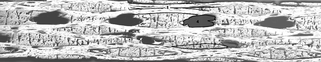
Figure 1: Representative segment of eight-layer plain weave fabric laminate.

Not only microstructural details but also properties of individual composite constituents have a direct impact on the quality of numerical predictions. Information supplied by manufacturers are, however, often insufficient. Moreover, the carbon matrix of the composite has properties dependent on particular manufacturing parameters such as the magnitude and durations of the applied temperature and pressure. Experimental derivation of some of the parameters is therefore needed. In connection with the elastic properties of the fiber and the matrix, the nanoindentation tests performed directly on the composite are discussed in Section 2.2 together with the determination of the necessary microstructural parameters mentioned already in the previous paragraphs.

Still, most of the work presented in this paper is computational. In particular, a brief summary of the procedure for the determination of the two-ply SEPUC for woven composites is given in Section 3. Section 4 is then reserved for the validation of the extracted geometrical and material parameters. To that end, the heat conduction and classical elasticity homogenization problems are compared with available experimental measurements. The concluding remarks are presented in Section 5.

2 Experimental program

As already stated in the introductory part, much of the considered here is primarily computational. However, no numerical predictions can be certified if not supported by proper experimental data [27]. Considering the mesoscopic complexity of C/C composites, the supportive role of experiments is assumed to have the following four components:

• Two-dimensional image analysis providing binary bitmaps of the composite further exploited in the derivation of a two-layer SEPUC.

• X-ray tomography yielding a three-dimensional map of distribution, shape and volume fraction of major pores to be introduced into a void-free SEPUC.

• Nanoindentation tests supplying the local material parameters which either depend on the manufacturing process or are not disclosed by the producer.

• Laboratory evaluation of effective properties both on micro and meso scales to support the experimental predictions. In the present study we adopt the experimental results available in [28] for effective elastic moduli and in [29] for effective thermal conductivities, see Section 4.2.

For the above purposes a carbon-polymer (C/P) laminated plate was first manufactured by molding together eight layers of carbon fabric Hexcel G 1169 composed of carbon multifilament Torayca T 800 HB and impregnated by phenolic resin Umaform LE. A set of twenty specimens having dimensions $25\times 2.5\times 2.5$ mm were then cut out of the laminate and subjected to further treatment (carbonization $C$ at 1000^∘C, reimpregnation $I$, recarbonization, second reimpregnation and final graphitization $G$ at 2200⁰C $(CICICG)$) to produce the carbon-carbon (C/C) composite. One particular illustration together with a binary representative appears in Figure 2.

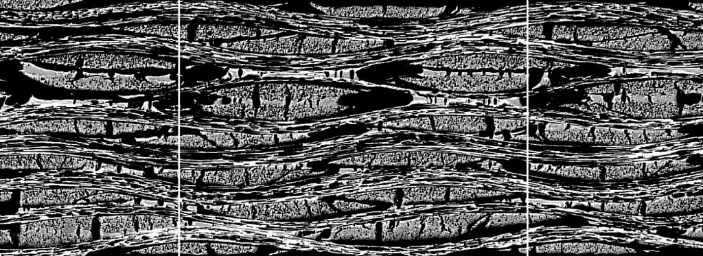
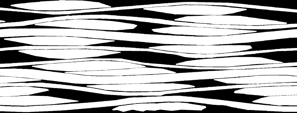
(a)	(b)

Figure 2: Examples of image analysis; (a) multi-layered C/C composite, (b) corresponding binary image

In the light of the first component of the experimental program, this composite was thoroughly studied in [30, 31] to yield basic structural parameters of a single-layer textile composite summarized in Table 1.

Table 1: Parameters of the periodic unit cell [30]

Parameter		Average	Standard deviation
Tow period	[$\mu$m]	4500	300
Tow height	[$\mu$m]	150	20
Inter-tow gap	[$\mu$m]	400	105
Layer height	[$\mu$m]	300	50
Horizontal shift	[$\mu$m]	0	675
Vertical shift	[$\mu$m]	0	110
Porosity	[%]	8	3.5
Pore aspect ratio	[-]	0.4	0.2

2.1 Three-dimensional X-ray microtomography

Porosity of C/C composites plays an important role in the derivation of effective material properties [32]. Although sectioning is typically used to characterize porosity from a two-dimensional images [31], the provided estimates of the porosity may significantly pollute the final predictions of the material response when compared to three-dimensional simulations [24]. The X-ray microtomography, rendering three-dimensional phase information directly, then becomes a valuable tool.

Apart from usual medical diagnostic applications, radiologic imaging is now commonly adopted in many other fields including material research, archeology, biology and other [33, 34]. For particular applications to woven composites the reader is referred to  [35, 36, 37].

The experimental measurements were carried out at the Institute of the Theoretical and Applied Mechanics, Academy of Sciences of the Czech Republic, employing the Microfocus X-ray source L8601-01 (Hamamatsu Photonics K.K.) with emission spot of $5~{}\mu$m and tungsten anode as the source of X-rays. For imaging, a large area X-ray detector C7942CA-22 (Hamamatsu Photonics K.K.) with resolution $2368\times 2240$ pixels and physical dimensions $120\times 120$ mm was used. To reduce the acquisition time $2\times 2$ pixel binning was adopted. The scanning sequence consisted of $720$ scans with $0.5^{\circ}$ step.

A spatial resolution of the resulting 3D images was $12~{}\mu$m³. A particular example of the reconstructed 3D image of C/P multi-layered plane-weave composite (green composite) together with the distribution of major porosity derived for the carbonized ($CICIC$) sample is presented in Figure 3. Note that for the green composite the major porosity amounted to $\approx 11\%$ while after several steps of reimpregnation and carbonization it was reduced to $\approx 8\%$, recall Table 1.

It is clear that these estimates are crucially dependent on the voxel resolution with respect to the pore size. Nevertheless, if considering the volume of an average pore equal to $100~{}\mu$m³ and accept the error of one voxel for each edge of the pore (a rectangular parallelepiped is assumed for simplicity), the error induced by calculation of the volume fraction of pores is less than $7\%$. Thus for the carbonized sample the error ($0.07\times 8\%=0.56\%$) will not exceed $1\%$ of the total volume.

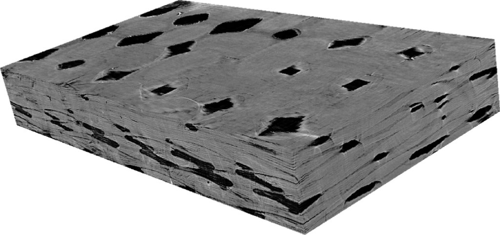
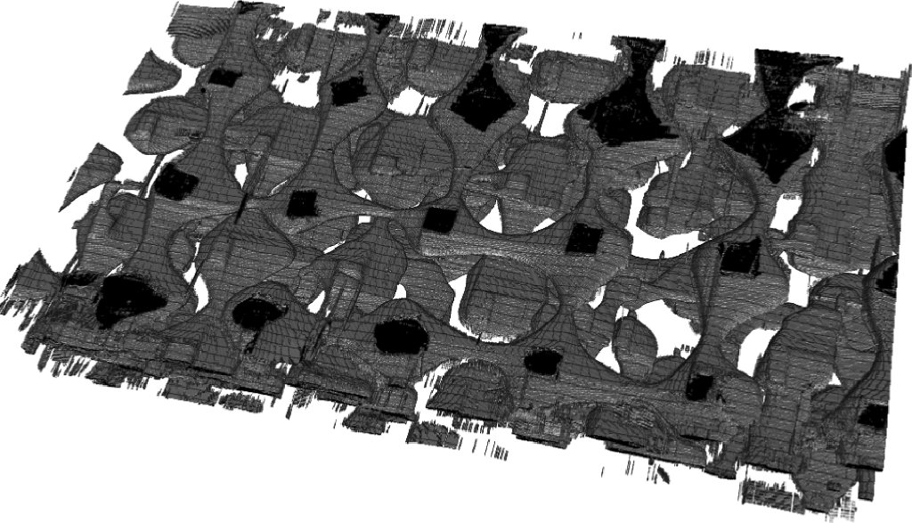
(a)	(b)

Figure 3: (a) Reconstructed 3D image of C/P composite, (b) reconstructed 3D image of porosity of C/C composite

2.2 Phase elastic moduli from nanoindentation

When predicting the effective behavior of composites from computations, we generally rely on information about material properties provided by the producer. Unfortunately, these are often insufficient for a three-dimensional analysis. It is also known that material properties of the matrix much depend on the fabrication of composite and may considerably deviate from those found experimentally for large unconstrained material samples [38]. Additional experiments, preferably performed directly on the composite, are therefore often needed to either validate the available local data or to derive the missing ones.

At present, nanoindentation is the only experimental technique that can be used for a direct measurement of mechanical properties at material micro-level. A successful application of nanoindentation to C/C composites has been reported in [39, 40, 41]. In the present text, our attention is limited to the evaluation of the matrix elastic modulus and the transverse elastic modulus of the fiber. The remaining data are assumed to be estimated from those available in the literature for similar material systems.

The reported measurements were performed at the Department of Mechanics of the Czech Technical University in Prague adopting the CSM Nanohardness tester. The testing head equipped with the Berkovich tip was coupled with an optical microscope ($5\times$ and $100\times$ optical magnifications) and CCD camera. The loading range of this equipment covers $0.1-500$ mN and the maximum penetration depth is $20$ $\mu$m.

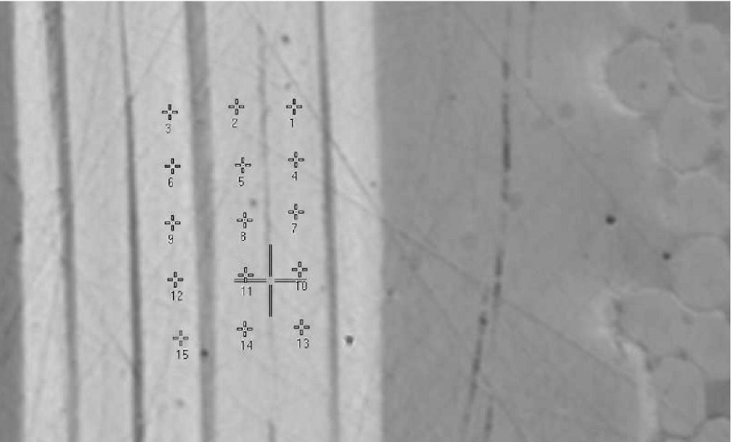
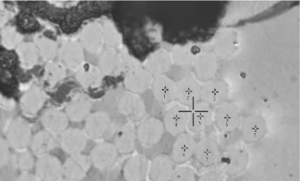
(a)	(b)

Figure 4: Nanoindentation - location of indents: (a) transverse direction, (b) perpendicular direction (compression)

Three locations, distinctly separated in optic microscope, were tested - matrix, parallel fibers Figure 4(a), perpendicular fibers Figure 4(b). The matrix was therefore assumed isotropic and possible anisotropy, which may arise inside the fiber tow, was not considered. As seen in Figure 4 several measurements were recorded for each of the three locations.

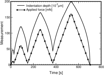
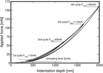
(a)	(b)

Figure 5: Measurements of matrix properties: (a) time variation of load and indentation depth, (b) indentation curves

The loading sequence for the matrix phase appears in Figure 5 showing the results for one particular indent, whereas for the fiber phase it is plotted in Figure 6 displaying several different indents.

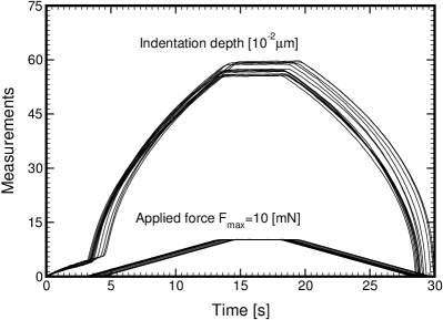
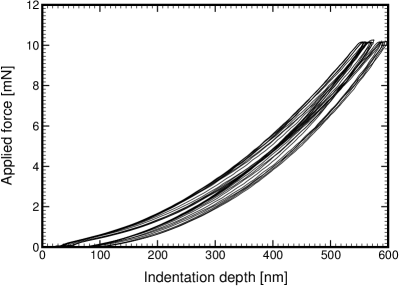
(a)	(b)

Figure 6: Measurements of fiber properties: (a) time variation of load and indentation depth, (b) indentation curves

As evident from Figs. 5(a) and  6(a), no creep was observed for both the matrix and and fibers as can be judged from no increase of an indentation depth for the period of constant load. Also note that the relative shift of individual indentation curves in Figure 6 caused by the difference of the onset of actual measurements is irrelevant (the measuring device introduces a non-zero indentation even before establishing a contact between the indenter and the measured sample, see the initial branches of the time variation of load and indentation depth in Figure 6(a)). The initial slope of the unloading part of indentation curves on the other hand plays a significant role when assessing the quality of measurements, since this branch is adopted to extract the elastic moduli [42] using the well known Oliver-Pharr procedure [43]. In this case, the unloading branch is almost identical for all measurements.

The complete set of material parameters, both measured averages labeled by ^∗ and those adopted from the literature, is available in Table 2. Note that the matrix modulus agrees relatively well with the one found for the glassy carbon in [41].

Table 2: Material parameters of individual phases

		Young modulus	Shear modulus	Poisson ratio
Material		[GPa]	[GPa]	[-]
fiber	longitudinal	294	11.8	0.24
	transverse	14.7∗	4.1	0.4
matrix		23.6∗	9.8	0.2

3 Statistically equivalent period unit cell

The concept of Statistically Equivalent Periodic Unit Cell (SEPUC) for random or imperfect microstructures is now well established. Individual steps, enabling the substitution of real microstructures by their simplified artificial representatives - the SEPUCs - are described, e.g. in [14, 1, 15] and additional references given below. Herein, these steps are briefly reviewed concentrating on the specifics of multi-layer woven composites.

3.1 Geometrical mesostructural model

The basic building block of the adopted SEPUC is provided by a single-ply model of plain weave composite geometry proposed by Kuhn and Charalambides in [44]. The model consists of two orthogonal warp and weft tows embedded in the matrix phase and it is parametrized by four basic quantities, directly measurable by two-dimensional image analysis (recall Table 1): the half-period of tow undulation $a$, the maximal tow thickness $b$, the width of the intra-tow gap $g$ and the overall height of the ply $h$, see Figure 7 (a). The three-dimensional woven composite SEPUC, shown in Figure 7 (b), is formed by two identical one-layer blocks, relatively shifted by distances $\Delta_{1}$, $\Delta_{2}$ and $\Delta_{3}$ in the direction of the corresponding coordinate axes. Finally, cutting a SEPUC by the plane $X_{2}=\pm a$ or $X_{1}=\pm a$ yields the warp or weft two-dimensional sections, used as the basis for the determination of the unit cell parameters.

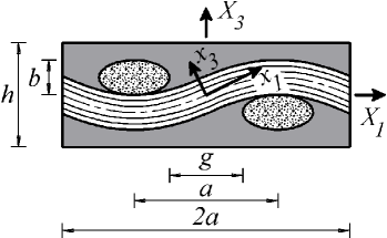
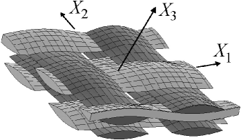
(a)	(b)

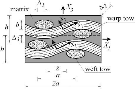
(c)

Figure 7: Geometrical model of SEPUC; (a) Two-dimensional cut of a one-layer model, (b) two-layer model including periodic extension of upper layer, (c) two-dimensional cut

3.2 Quantification of random microstructure

Assuming a statistically homogeneous and ergodic binary material system, two basic statistical functions are available to capture essential characteristics of the analyzed tow-matrix material system. The first descriptor is a two-point probability function $S(\mbox{\boldmath$X$})$ [45], which quantifies the probability of two points, separated by a vector $X$, being both found in the domain occupied by the warp and weft tows. The alternative statistics, proposed by Lu and Torquato [46] to capture long-range effects, is the linear path function $L(\mbox{\boldmath$X$})$ giving the probability that a randomly placed segment $X$ is fully contained in the tow region. Both descriptors can be easily computed for digitized microstructures; in particular, the Fast Fourier transform library FFTW [47] is used to evaluate the $S$ function and the sampling template consisting of $N_{d}$ concentric rays discretized by $N_{\ell}$ pixels (cf. Figure 8) is employed to determine the linear path function. The periodic boundary conditions were adopted for both descriptors to eliminate edge effects [48].

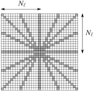
Figure 8: Example of sample template for lineal path function generated by $N_{d}=16$ segments, each of which is discretized using $N_{\ell}=17$ pixels.

3.3 Calibration of SEPUC parameters

In overall, the adopted model of the unit cell involves seven independent parameters

$$\mbox{\boldmath$y$}=\left[a,b,g,h,\Delta_{1},\Delta_{2},\Delta_{3}\right],$$ (1)

to be determined from available microstructural data. For the sake of generality, we assume that the microstructure configuration is characterized by microstructural function associated with (at most) warp and weft directions; i.e. functions $S_{\sf{warp}}$ and $L_{\sf{warp}}$ for the warp cross-section and descriptors $S_{\sf{weft}}$ and $L_{\sf{weft}}$ for the weft cross-section, recall Figure 7(b). In particular, see also [15, 16], the following quantities are introduced to measure the similarity between a SEPUC and the original microstructure:

$$F_{S}^{2}(\mbox{\boldmath$y$}) = \frac{1}{i_{\rm max}j_{\rm max}}\sum_{p\in\{\sf{warp},\sf{weft}\}}\sum_{i=-i_{\rm max}}^{i_{\rm max}}\sum_{j=-j_{\rm max}}^{j_{\rm max}}\left(S_{p}(\mbox{\boldmath$y$},i,j)-\overline{S}_{p}(i,j)\right)^{2},$$ (2)

$$F_{L}^{2}(\mbox{\boldmath$y$}) = \frac{1}{N_{d}N_{\ell}}\sum_{p\in\{\sf{warp},\sf{weft}\}}\sum_{i=1}^{N_{d}}\sum_{j=1}^{N_{\ell}}\left(L_{p}(\mbox{\boldmath$y$},i,j)-\overline{L}_{p}(i,j)\right)^{2},$$ (3)

where, e.g. $S_{\sf{warp}}(\mbox{\boldmath$y$},i,j)$ denotes the two-point probability function determined for the warp cross-section of a SEPUC described by parameters $y$ and the value of argument $\mbox{\boldmath$X$}=[i,j]$, $L_{\sf{weft}}(\mbox{\boldmath$y$},i,j)$ stores the value of the weft-section lineal path function for the $j$-th pixel of the $i$-th segment, $\overline{S}_{\bullet}$ and $\overline{L}_{\bullet}$ denote the statistics related to original media and the dimensions $i_{\rm max}$ and $j_{\rm max}$ are determined as half of the minimum height and width of the bitmaps representing a SEPUC and the reference image.

The two-dimensional data can be complemented by independent experimental measurements of three-dimensional volume fractions of the tow phase, see [31] for further details. Such information is accounted for by an additional discrepancy measure

$$F_{\phi}(\mbox{\boldmath$y$})=|\phi(\mbox{\boldmath$y$})-\overline{\phi}|,$$ (4)

where $\phi(\mbox{\boldmath$y$})$ denotes the SEPUC three-dimensional volume fraction and $\overline{\phi}$ is the target value. The former quantity is determined from the analytical representation of the SEPUC geometry [44] using an adaptive Simpson quadrature [49, Chapter 4] with the relative accuracy set to $10^{-5}$.

Moreover, the multiple descriptors can be arbitrary combined in the form of a weighted sum. For example, if all available information is employed, the objective function attains the form

$$F_{S+L+\phi}(\mbox{\boldmath$y$})=\alpha_{S}F_{S}(\mbox{\boldmath$y$})+\alpha_{L}F_{L}(\mbox{\boldmath$y$})+\alpha_{\phi}F_{\phi}(\mbox{\boldmath$y$}),$$ (5)

with $\alpha_{\bullet}$ denoting scale factors used to normalize the influence of each descriptor, determined from twenty randomly generated SEPUCs in the current study.

The final term is introduced into the objective function to eliminate the intersection of the upper-layer and lower-layer tows. To that end, we compute the overlap $\delta$ as the minimum signed distance between the upper and lower tow surfaces and introduce the constraint $\delta\geq 0$ via a polynomial exterior penalty:

$$f_{D}(\mbox{\boldmath$y$})=\left(1+\frac{\delta_{-}(\mbox{\boldmath$y$})}{h}\right)^{\beta}F_{D}(\mbox{\boldmath$y$}),$$ (6)

where $\delta_{-}$ denotes the negative part of $\delta$, $D$ refers to a particular combination of the descriptors and the value of exponent is set to $\beta=3$. Note that this approach was inspired by work of Collins et al. [50] related to high-density polydisperse particulate composites.

Now, the optimal values of the SEPUC parameters can be determined as the solution to a box-constrained global optimization problem

$$\mbox{\boldmath$y$}\in\operatorname*{Argmin}_{\mbox{\boldmath$l$}\leq\mbox{\boldmath$z$}\leq\mbox{\boldmath$u$}}f_{D}(\mbox{\boldmath$z$}),$$ (7)

where the lower and upper bounds $l$ and $u$ are directly linked to standard deviations in Table 1 acquired from two-dimensional image analysis. A closer inspection reveals that objective functions (6) are multi-modal and discontinuous due to the effect of limited bitmap resolution, cf. [51]. Based on our previous experience with evolutionary optimization, a stochastic optimization algorithm RASA [52, 53], based on a combination of a real-valued genetic algorithm and the Simulated Annealing method, is used to solve the optimization problem (7).

3.4 SEPUC for multi-layered C/C composite

This section is concerned with the analysis of the eight-layer C/C composite represented by the bitmap appearing in Figure 2(c). First, to keep the optimization process manageable, the original $2,261\times 861$ bitmap was down-sampled to a $1,024\times 390$ image, resulting in the pixel size of $4.4~{}\mu$m. In accordance with conclusions of the previous section, all available information was employed to determine SEPUC parameters, constrained to the range $\overline{y}_{i}\pm 3\sigma_{i}$, with $\overline{y}_{i}$ and $\sigma_{i}$ denoting the mean and the standard deviation of the $i$-th structural parameter taken from Table 1. Parameters of the algorithm were set to the identical values as in [51, page 65] and the termination criterion was set to $50,000$ of $f_{S+L+\phi}$ function evaluations. The optimization was executed independently twenty times to obtain reliable results.

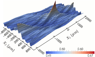
(a)

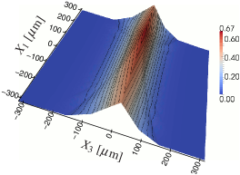
(b)

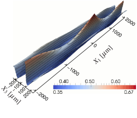
(c)

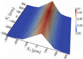
(d)

Figure 9: Statistical descriptors for multi-layered C/C composite and SEPUC; (a) two-point probability function and (b) lineal path function determined for multi-layered composite, (c) two-point probability function and (d) lineal path function corresponding to SEPUC

The resulting two-point and lineal-path functions corresponding to the SEPUC and the original microstructure appear in Figure 9. In the $X_{1}$-axis direction, the original statistics is well-reproduced, particularly at the $X_{3}=0~{}\mu$m plane where the extreme values and the shape of the descriptors are in almost perfect agreement. The SEPUC also partially captures the local peaks appearing in the multi-layer system for $X_{3}\approx\pm 200~{}\mu$m, cf. Figure 9 (a). In the perpendicular direction, we observe that the SEPUC two-point probability function is influenced by periodic boundary conditions, leading to more oscillatory behavior and to a slight shift of the minimum values from $41\%$ to $35\%$. The match between the lineal path functions in terms of extreme values and shape of the function is even closer, since this descriptor is non-periodic even for periodic microstructures. Finally note that the tree-dimensional volume fraction $\phi$ of the SEPUC is $51\%$, which coincides exactly with the reference value taken from [31]. Therefore, we conjecture that the idealized SEPUC captures the dominant geometrical features of the original system; the differences visible from Figure 9 arise mainly due to the periodic boundary conditions and idealized shape of SEPUC.

In Table 3, we present the parameters of the SEPUC together with the standard deviations estimated from independent optimization runs. The scatter in the identified parameters is mainly induced by discretization errors and does not exceed three pixel sizes. The values of the parameters demonstrate that SEPUC captures a moderate horizontal shift of individual layers and their mutual overlap. These conclusions are further supported by a three-dimensional representation in Figure 10(b) and Figure 14, showing that SEPUC reproduces the matrix rich regions together with the strong nesting of individual layers, of course within the constraints of the selected geometrical model and the tow impenetrability condition.

Table 3: Optimal parameters of the two-layer periodic unit cell free of pores; numbers in parentheses correspond to standard deviations

$a$ [$\mu$m]	$b$ [$\mu$m]	$g$ [$\mu$m]	$h$ [$\mu$m]	$\Delta_{1}=\Delta_{2}$ [$\mu$m]	$\Delta_{3}$ [$\mu$m]
$2,181$	$118$	$394$	$251$	$288$	$-47$
($10.0$)	($0.3$)	($0.1$)	($1.3$)	($10.5$)	($2.0$)

3.5 Computational model

A crucial step in the successful calculation of effective properties is the finite element discretization of SEPUC. This step typically implies the use of conforming finite element meshes [6] enabling the implementation of periodic boundary conditions by assigning the same code numbers to homologous nodes on opposite sides of a rectangular unit cell [54, 14]. Such meshes are also expected to explicitly resolve all heterogeneities so that only one phase is present in each finite element. In case of the two layer SEPUC these include not only the warp and weft tow boundaries but also the boundary of major voids. Based on the results provided by X-ray microtomography we assumed disordered voids created by coating each fiber tow with a layer of matrix such that the volume of coating complies with the respective volume fraction of the matrix phase. The remaining space of the total volume of SEPUC then devolves upon the porous phase.

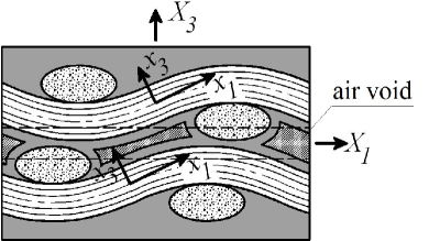
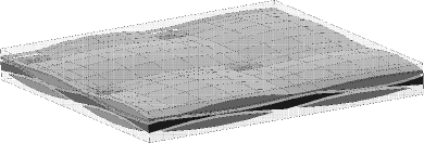
(a)	(b)

Figure 10: (a) Two-dimensional cut of a two-layer model with distorted voids (b) 3D view of the geometry of a two-layer UC model with distorted voids

As evident from Figure 10 relatively sharp areas at fiber-tow crossings may lead to inappropriately distorted elements if attempting to match all geometrical boundaries. To avoid such complications we adopt the approach based on the extended finite element method (X-FEM), which allows us to treat complex geometries relatively easily. More specifically, the method enables an application of regular meshes, which do not have to confirm to physical boundaries. These are captured by enriching the approximation space of the finite element with embedded interface exploiting the partition of unity technique. In the present context, the theoretical formulation described by Moës et al. [26] will be pursued.

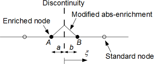
Figure 11: Modified abs-enrichment for 1D problem.

To introduce the subject, consider a one-dimensional problem in Figure 11 with an element AB crossed by a material discontinuity. The principal idea of X-FEM is to augment the standard approximation space of the displacements or temperatures with a specific enrichment function $\psi(\boldsymbol{X})$ which renders the corresponding gradients discontinuous along the material interface. Following [26] and for simplicity limiting attention to the heat conduction case the augmented approximation of the temperature field reads

$${\theta}(\boldsymbol{X})=\sum_{i\in I}{N}_{i}(\boldsymbol{X}){\theta}_{i}+\sum_{j\in I^{*}}{N}_{j}^{*}(\boldsymbol{X})\psi(\boldsymbol{X}){a}_{j},$$ (8)

where ${N}_{i}$ are the standard shape functions, $I$ represents the total number of finite element nodes in the analyzed domain, $I^{*}\subset I$ gives the number of nodes for which the support is split by the interface and ${a}_{j}$ are the additional degrees of freedom. To properly capture the interface location within an element Sukumar et al. [25] applied a level set representation of surfaces through a level set function

$$\phi(\boldsymbol{X})=\sum_{i\in J}{N}^{*}_{i}(\boldsymbol{X})\boldsymbol{\phi}_{i},$$ (9)

where ${N}^{*}_{i}$ are the shape functions building a local partition of unity, in most cases ${N}^{*}_{i}={N}_{i}$. Then, $J$ stands for the number of nodes of the element for temperature discretization containing the point $\boldsymbol{X}$. The nodal values $\boldsymbol{\phi}_{i}$ represent the signed distance of the element node to the interface with either a positive or a negative value depending on the material to which it belongs as sketched in Figure 12(a). This function then locates interfaces implicitly as a union of points for which it attains a zero value (zero-level). An example of a level set function for a square plate with an embedded hole is shown in Figure 12(c). The situation in which two interfaces of the same material phase are found in a given element, see Figure 12(b), should be avoided since the resulting approximation would not yield the iso-zero of the level set function inside the element correctly. This condition thus calls for a minimum mesh refinement at least locally in the vicinity of two interfacases of the same material, i.e. interfaces defined by the same level set function.

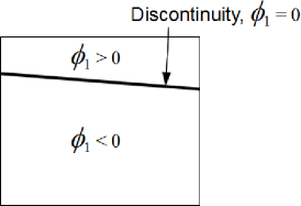
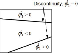
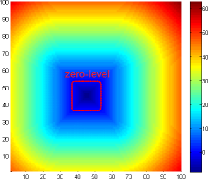
(a)	(b)	(c)

Figure 12: Representation of the level set function function: (a) element crossed by a single material interface, (b) element crossed by two interfaces of the same material phase, (c) example of the level set function for a square plate with a hole

Given the level set function, Moës et al. [26] introduced a specific form of the enrichment function in the form

$$\psi(\boldsymbol{X})=\sum_{i\in J}\left|\phi_{i}\right|{N}_{i}^{*}(\boldsymbol{X})-\left|\sum_{i\in J}\phi_{i}{N}_{i}^{*}(\boldsymbol{X})\right|,$$ (10)

where $\phi_{i}$ denotes the level set value in the node $i$. Note that the actual value of $\psi$ along the interface is irrelevant as long as it captures the weak discontinuity in gradient fields properly. For the general case of $K$ enrichment we get

$${\theta}(\boldsymbol{X})=\sum_{i=1}^{I}{N}_{i}(\boldsymbol{X}){\theta}_{i}+\sum_{k=1}^{K}\sum_{j\in J_{k}}{N}_{j}^{*}(\boldsymbol{X})\psi(\boldsymbol{X})^{k}{a}_{j}^{k},$$ (11)

where $J_{k}$ stands for a nodal subset of the enrichment $k$. In the elasticity case Eq. (11) applies to each component of the local displacement field $\boldsymbol{u}(\boldsymbol{X})$. Notice that for the analyzed porous textile composites three enrichment functions might arise for a single element associated in turn with the weft and warp tows and a void.

Several issues worth of noting arise with numerical implementation. The first two are general and include proper numerical integration and application of periodic boundary conditions as discussed in [55] and [26], respectively.

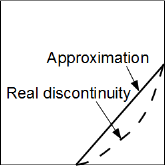
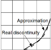
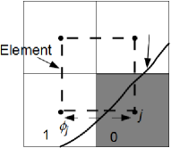
(a)	(b)	(c)	(d)

Figure 13:

Other issues are concerned with the approximation of shape and location of a real interface. The accuracy depends on the interpolation of the level set function, typically on the finite element mesh, and evaluation of the sign distances $\phi_{j}$. It can be expected that the finer the mesh the smaller the geometrical error will be. This is demonstrated in Figs. 13(a)(b) for the case of a linear interpolation of the level set function which intrinsically replaces a curved interface by a straight line in 2D or a plane in 3D problems. To measure the sign distances $\phi_{j}$, we adopted a binary representation of the geometrical model instead of using explicit definition of individual interfaces, which for the porous phase would be rather complicated.

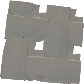
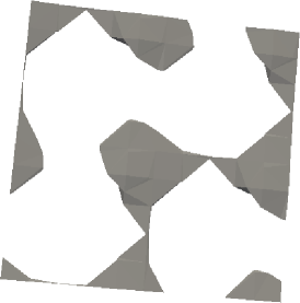
(a)	(b)
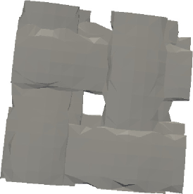
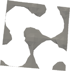
(c)	(d)
(e)	(f)

Figure 14: Iso-zero representation of fiber-tows and a porous phase of the SEPUC in Figure 10 based solely on the finite element approximation for three regular meshes: (a,b) $10\times{10}\times{8}$, (c,d) $15\times{15}\times{10}$, (e,f) $20\times{20}\times{15}$

The images were created consecutively for the three material phases (fiber-tow in warp and weft directions and voids) starting with the resolution corresponding to the underlying uniform finite element mesh. For each interface the value of $\phi_{j}$ was defined as a distance of the zero-value pixel associated with the node $j$ to the nearest non-zero pixel as seen in Figure 13(c). Notice that element nodes are imagined in the centers of pixels. To receive more accurate results each cube can be further subdivided into smaller parts (pixels) as displayed in Figure 13(d).

The need for sufficiently fine meshes to accurately locate the material interfaces becomes particularly important in the light of volume fractions of individual phases, which play a crucial role in the actual predictions of effective properties. Figure 14 displays the iso-zero level set separately for the fiber-tows and the porous phase for the selected three meshes of different refinement. One should notice, apart from an improved representation of the interface location, the change in volume of individual phase.

Table 4: Mesh properties and associate phase volume fractions

Mesh	Conforming	Uniform (X-FEM)
	(FEM)	$20\times{20}\times{15}$	$15\times{15}\times{10}$	$10\times{10}\times{8}$
$\#$ elements	69169	6000	2250	800
$\#$ equations	11696	15148	6893	2726
$\#$ int.points	69169	182340	103076	40372
$c_{m}$	0.431	0.451	0.495	0.553
$c_{f}$	0.497	0.484	0.456	0.409
$c_{p}$	0.071	0.065	0.050	0.038

Table 4 provides summary on individual finite element meshes. The corresponding results attributed to a conforming mesh are also listed for comparison. Clearly, further refinement would be needed in both the X-FEM and standard formulation to arrive at $8$% porosity measured by X-ray microtomography. The actual distribution of porosity plotted in Figure 3(b) is, however, captured by X-FEM approximation relatively well. This issue will yet be commented on in Section 4.2 when discussing the results of numerical analysis.

4 Numerical evaluation of effective properties

Numerical evaluation of effective elastic moduli and thermal conductivities, the most classical subject in micromechanics, is descried in this section in support of the proposed concept of SEPUC applied to multi-layered C/C composites. This selection of mechanical and heat conduction problem is promoted not only by available experimental measurements but also by their formal similarity, considerably simplifying the theoretical treatment as seen hereinafter.

4.1 Theoretical formulation of homogenization

First-order homogenization approaches are now well established and described in many papers [54, 56, to cite a few] to provide estimates of effective properties of material systems with periodic microstructures. Bearing in mind the analogy between basic quantities related to heat conduction problems (i.e. the local microscopic $\mbox{\boldmath$h$}(\mbox{\boldmath$x$})$ and uniform macroscopic $H$ temperature gradients and fluxes $\mbox{\boldmath$q$}(\mbox{\boldmath$x$})$ and $Q$ as their conjugate measures) and the corresponding quantities applied to mechanical problems (local $\mbox{\boldmath$\varepsilon$}(\mbox{\boldmath$x$})$ and uniform $E$ strains and the conjugate stress measures $\mbox{\boldmath$\sigma$}(\mbox{\boldmath$x$})$ and $\Sigma$), we consider a heterogeneous periodic unit cell $Y$ and variations of local temperature $\theta(\mbox{\boldmath$X$})$ and displacement $\mbox{\boldmath$u$}(\mbox{\boldmath$X$})$ fields written in terms of the uniform macroscopic quantities $H$ and $E$ as

$$\theta(\mbox{\boldmath$X$})=\mbox{\boldmath$H$}\cdot\mbox{\boldmath$X$}+\theta^{*}(\mbox{\boldmath$X$}),\hskip 42.67912pt\mbox{\boldmath$u$}(\mbox{\boldmath$X$})=\mbox{\boldmath$E$}\cdot\mbox{\boldmath$X$}+\mbox{\boldmath$u$}^{*}(\mbox{\boldmath$X$}),$$ (12)

where $\theta^{*}$ and $\mbox{\boldmath$u$}^{*}$ are $Y$-periodic temperature and displacements fluctuations, respectively and $\bullet(\mbox{\boldmath$X$})$ is introduced to represent a given quantity in the global coordinate system $X$, recall Figure 7. Next, denoting $\mbox{\boldmath$\chi$}(\mbox{\boldmath$x$})$ the local conductivity matrix and similarly ${\mathbf{L}}(\mbox{\boldmath$x$})$ the local stiffness matrix, the local microscopic constitutive equations in the local coordinate system $x$ become

$$\mbox{\boldmath$q$}(\mbox{\boldmath$x$})=-\mbox{\boldmath$\chi$}(\mbox{\boldmath$x$})\mbox{\boldmath$h$}(\mbox{\boldmath$x$}),\hskip 42.67912pt\mbox{\boldmath$\sigma$}(\mbox{\boldmath$x$})={\mathbf{L}}(\mbox{\boldmath$x$})\mbox{\boldmath$\varepsilon$}(\mbox{\boldmath$x$}).$$ (13)

To complete the set of equations needed in the derivation of effective properties, we recall the Hill lemma for mechanical problem and the Fourier inequality [57] for an equivalent representation of steady state heat conduction problem together with Eqs. (13) and write the global-local variational principles, see e.g. [23, 58, for further details] in the forms

$$\left\langle\delta\mbox{\boldmath$h$}(\mbox{\boldmath$x$}){\sf{}^{T}}\mbox{\boldmath$\chi$}(\mbox{\boldmath$x$})\mbox{\boldmath$h$}(\mbox{\boldmath$x$})\right\rangle=0,\hskip 42.67912pt\left\langle\delta\mbox{\boldmath$\varepsilon$}(\mbox{\boldmath$x$}){\sf{}^{T}}{\mathbf{L}}(\mbox{\boldmath$x$})\mbox{\boldmath$\varepsilon$}(\mbox{\boldmath$x$})\right\rangle=0,$$ (14)

where $\left\langle a(\mbox{\boldmath$x$})\right\rangle$ represents the volume average of a given quantity, i.e. $\left\langle a(\mbox{\boldmath$x$})\right\rangle=\frac{1}{|\Omega|}\int_{\Omega}a(\mbox{\boldmath$x$})\,{\mathrm{d}}\Omega$. In the framework of finite element approximation, the discrete forms of local gradients derived from Eqs. (12) read

$$\mbox{\boldmath$h$}(\mbox{\boldmath$X$})=\mbox{\boldmath$H$}+{\mathbf{B}}^{\theta}(\mbox{\boldmath$X$})\mbox{\boldmath$\theta$}^{*}_{d},\hskip 42.67912pt\mbox{\boldmath$\varepsilon$}(\mbox{\boldmath$X$})=\mbox{\boldmath$E$}+{\mathbf{B}}^{u}(\mbox{\boldmath$X$})\mbox{\boldmath$u$}^{*}_{d},$$ (15)

where ${\mathbf{B}}^{\bullet}$ stores the derivatives of the element shape functions w.r.t. $X$ and $\mbox{\boldmath$\theta$}^{*}_{d}$ and $\mbox{\boldmath$u$}^{*}_{d}$ are the vectors of the fluctuation part of nodal temperatures and displacements, respectively. Substituting Eqs. (15) into Eqs. (14) gives

$$\delta\mbox{\boldmath$\theta$}^{*}_{d}{\sf{}^{T}}\left\langle{\mathbf{B}}^{\theta}(\mbox{\boldmath$X$}){\sf{}^{T}}\mbox{\boldmath$\chi$}(\mbox{\boldmath$X$}){\mathbf{B}}^{\theta}(\mbox{\boldmath$X$})\right\rangle\mbox{\boldmath$\theta$}^{*}_{d} = -\delta\mbox{\boldmath$\theta$}^{*}_{d}{\sf{}^{T}}\left\langle{\mathbf{B}}^{\theta}(\mbox{\boldmath$X$}){\sf{}^{T}}\mbox{\boldmath$\chi$}(\mbox{\boldmath$X$})\right\rangle\mbox{\boldmath$H$},$$ (16)

$$\delta\mbox{\boldmath$u$}^{*}_{d}{\sf{}^{T}}\left\langle{\mathbf{B}}^{u}(\mbox{\boldmath$X$}){\sf{}^{T}}{\mathbf{L}}(\mbox{\boldmath$X$}){\mathbf{B}}^{u}(\mbox{\boldmath$X$})\right\rangle\mbox{\boldmath$u$}^{*}_{d} = -\delta\mbox{\boldmath$u$}^{*}_{d}{\sf{}^{T}}\left\langle{\mathbf{B}}^{u}(\mbox{\boldmath$X$}){\sf{}^{T}}{\mathbf{L}}(\mbox{\boldmath$X$})\right\rangle\mbox{\boldmath$E$},$$ (17)

to be solved for nodal temperatures $\mbox{\boldmath$\theta$}^{*}_{d}$ and nodal displacements $\mbox{\boldmath$u$}^{*}_{d}$. Combining Eqs. (15) and Eqs. (13) now allows us to write the volume averages of local heat fluxes and local stresses as

$$Q = \left\langle{\mathbf{T}}^{\theta}(\mbox{\boldmath$X$}){\sf{}^{T}}\mbox{\boldmath$q$}(\mbox{\boldmath$x$})\right\rangle\,=\,-\frac{1}{|\Omega|}\int_{\Omega}{\mathbf{T}}^{\theta}(\mbox{\boldmath$X$}){\sf{}^{T}}\mbox{\boldmath$\chi$}(\mbox{\boldmath$x$}){\mathbf{T}}^{\theta}(\mbox{\boldmath$X$})\mbox{\boldmath$h$}(\mbox{\boldmath$X$})\,{\mathrm{d}}\Omega,$$ (18)

$$\Sigma = \left\langle{\mathbf{T}}^{\mbox{\boldmath$\varepsilon$}}(\mbox{\boldmath$X$}){\sf{}^{T}}\mbox{\boldmath$\sigma$}(\mbox{\boldmath$x$})\right\rangle\,=\,\frac{1}{|\Omega|}\int_{\Omega}{\mathbf{T}}^{\mbox{\boldmath$\varepsilon$}}(\mbox{\boldmath$X$}){\sf{}^{T}}{\mathbf{L}}(\mbox{\boldmath$x$}){\mathbf{T}}^{\mbox{\boldmath$\varepsilon$}}(\mbox{\boldmath$X$})\mbox{\boldmath$\varepsilon$}(\mbox{\boldmath$X$})\,{\mathrm{d}}\Omega,$$ (19)

also showing the relationship between material matrices in the local and global coordinate systems in terms of transformation matrices ${\mathbf{T}}^{\theta},{\mathbf{T}}^{\mbox{\boldmath$\varepsilon$}}$, see e.g. [59, 51, 23, 24],

$$\mbox{\boldmath$\chi$}(\mbox{\boldmath$X$})={\mathbf{T}}^{\theta}(\mbox{\boldmath$X$}){\sf{}^{T}}\mbox{\boldmath$\chi$}(\mbox{\boldmath$x$}){\mathbf{T}}^{\theta}(\mbox{\boldmath$X$}),\hskip 42.67912pt{\mathbf{L}}(\mbox{\boldmath$X$})={\mathbf{T}}^{\mbox{\boldmath$\varepsilon$}}(\mbox{\boldmath$X$}){\sf{}^{T}}{\mathbf{L}}(\mbox{\boldmath$x$}){\mathbf{T}}^{\mbox{\boldmath$\varepsilon$}}(\mbox{\boldmath$X$}).$$ (20)

The results of Eqs. (18) and (19) renders the macroscopic constitutive laws in the form

$$\mbox{\boldmath$Q$}=-\mbox{\boldmath$\chi$}^{\sf H}\mbox{\boldmath$H$},\hskip 42.67912pt\mbox{\boldmath$\Sigma$}={\mathbf{L}}^{\sf H}\mbox{\boldmath$E$},$$ (21)

where $\mbox{\boldmath$\chi$}^{\sf H}$ and ${\mathbf{L}}^{\sf H}$ are the searched homogenized effective thermal conductivity and elastic stiffness matrices, respectively. In particular, for a three-dimensional SEPUC the components of the $3\times 3$ conductivity matrix $\mbox{\boldmath$\chi$}^{\sf H}$ follow directly from the solution of three successive steady state heat conduction problems. To that end, the periodic unit cell is loaded, in turn, by each of the three components of $H$, while the other two vanish. The volume flux averages, Eq. (18), normalized with respect to $H$ then furnish individual columns of $\mbox{\boldmath$\chi$}^{\sf H}$. The components of the $6\times 6$ elastic stiffness matrix ${\mathbf{L}}^{\sf H}$ are found analogously from the solution of six independent elasticity problems together with Eq. (19).

4.2 Numerical simulations

In the framework of hierarchical modeling the analysis proceeded in two steps. First, the effective elastic properties of a porous yarn were estimated using the Mori-Tanaka [60] averaging scheme and the local properties stored in Table 2. The results appear in Table 5 showing a good agreement with experimental values taken from [28].

Table 5: Effective elastic properties of unidirectional C/C composite (porous fiber tow) and C/C laminate moduli [28] given in [GPa]

parameter	porous tow (MT)	porous tow (EXP)	C/C laminate (EXP)
$E_{11}$	193.8	$\approx$ 200	$\approx$ 65
$G_{12}$	10.3	$\approx$ 11.5	$\approx$ 6

This encouraging result promoted the application of the Mori-Tanaka method also in the derivation of effective thermal conductivities. Both local phase conductivities and the resulting estimates of effective properties of a porous yarn are available in Table 6. Since providing the theoretical details of the Mori-Tanaka method goes beyond the present scope, we suggest the interested reader to consult our recent work on this subject [12, 24] emphasizing the applicability of the Mori-Tanaka method also in the field of imperfect textile composites.

The second step involved application of the 1st order homogenization discussed in the previous section and the computational model developed in Section 3.5. The corresponding results are given Table 7. The table shows how the X-FEM results converge with the uniform mesh refinement to those attributed to a conforming mesh.

Table 6: Phase [31], unidirectional C/C composite (porous fiber tow) and laminate effective thermal conductivities [29]

material	Thermal conductivities [Wm-1K-1]
	$\chi_{11}$	$\chi_{22}$	$\chi_{33}$
air	0.02	0.02	0.02
fiber	35	0.35	0.35
matrix	6.3	6.3	6.3
porous tow (MT)	24.12	1.05	1.42
C/C laminate (EXP)	10 ($\sf{warp}$)	10 ($\sf{weft}$)	1.6

The most pronounced discrepancies, when compared to standard FEM computations exploiting conforming meshes, clearly follow from an inaccurate representation of major porosity when coarse meshes are used. This is also evidenced by plots of the porous phase in Figure 14 and the corresponding error in the estimated volume fractions in Table 4. However, given the complexity of multi-scale analysis, the theoretical predictions when compared to experimental data listed also in Table 5 and Table 6 still provide reasonable confidence in the proposed approach strongly relying on the concept of statistically equivalent periodic unit cell.

Table 7: Comparison of X-FEM and FEM predictions for heat conduction and linear elasticity problem

Problem		Conforming	Uniform X-FEM
properties		FEM (EXP)	$20\times{20}\times{15}$	$15\times{15}\times{10}$	$10\times{10}\times{8}$
Conduction	$\chi_{11}$	8.81 (10)	8.85	8.74	8.52
$[$Wm-1K${}^{-1}]$	$\chi_{33}$	1.31 (1.6)	1.81	2.15	2.61
Elasticity	$E_{11}$	58.75 (65)	58.53	56.73	53.53
$[$GPa$]$	$E_{33}$	8.18	13.41	15.51	17.47
	$G_{23}$	3.64	5.19	5.93	6.72
	$G_{12}$	7.86 (6)	7.99	8.17	8.41
$[-]$	$\nu_{23}$	0.05	0.05	0.06	0.06
	$\nu_{12}$	0.03	0.06	0.07	0.08

5 Conclusions

The present article summarizes recent developments in the study of imperfect carbon-carbon textile composites initiated already in 2004 in part I [1] of this series. To arrive at the present stage of understanding of the complex structural response of these material systems, the machinery of homogenization tools has been fully exploited.

In view of real material samples impaired by a large amount of flaws (transverse and delamination cracks, large intertow vacuoles) even prior to loading, the modeling strategy based on the well known concept of periodic unit cell may become preferable, particularly if the response of the material exceeding its elastic limit [61, 62, 63] is the primary interest. Presently, its potential is seen mainly in the formulation of statistically equivalent periodic unit cell that attempts to accommodate the most severe imperfections of the real material. Supported by the results derived in the course of this work, the two-layer SEPUC enhanced by incorporating the porous phase appears to be a suitable candidate for the computational model of plain weave textile reinforcement based composites including, apart from the investigated C/C composites, a large group of textile reinforced ceramics with their anticipated application in bio-medicine.

References

- [1] J. Zeman, M. Šejnoha, Homogenization of balanced plain weave composites with imperfect microstructure: Part I–Theoretical formulation, International Journal of Solids and Structures 41 (22-23) (2004) 6549–6571.
- [2] B. Cox, Q. Yang, In quest of virtual tests for structural composites, Science 314 (5802) (2006) 1102–1107.
- [3] B. N. Cox, G. Flanagan, Handbook of analytical methods for textile composites, Tech. rep., NASA Contractor Report 4750, Langley Research Center (1997).
- [4] P. W. Chung, K. K. Tamma, Woven fabric composites - developments in engineering bounds, homogenization and applications, International Journal for Numerical Methods in Engineering 45 (12) (1999) 1757–1790.
- [5] S. V. Lomov, D. S. Ivanov, I. Verpoest, M. Zako, T. Kurashiki, H. Nakai, S. Hirosawa, Meso-FE modelling of textile composites: Road map, data flow and algorithms, Composites Science and Technology 67 (9) (2007) 1870–1891.
- [6] R. Wentorf, R. Collar, M. S. Shephard, J. Fish, Automated modeling for complex woven mesostructures, Computer Methods in Applied Mechanics and Engineering 172 (1–4) (1999) 273–291.
- [7] G. Hivet, P. Boisse, Consistent 3D geometrical model of fabric elementary cell. Application to a meshing preprocessor for 3D finite element analysis, Finite Elements in Analysis and Design 42 (1) (2005) 25–49.
- [8] E. J. Barbero, T. J., J. A. Mayugo, K. K. Sikkil, Finite element modeling of plain weave fabrics from photomicrograph measurements, Composite Structures 73 (1) (2005) 41–52.
- [9] C. M. Pastore, Quantification of processing artifacts in textile composites, Composites Manufacturing 4 (4) (1993) 217–226.
- [10] S. Yurgartis, K. Morey, J. Jortner, Measurement of yarn shape and nesting in plain-weave composites, Composites Science and Technology 46 (1) (1993) 39–50.
- [11] S. P. Yushanov, A. E. Bogdanovich, Stochastic theory of composite materials with random waviness of the reinforcements, International Journal of Solids and Structures 35 (22) (1998) 2901–2930.
- [12] J. Skoček, J. Zeman, M. Šejnoha, Effective properties of Carbon-Carbon textile composites: application of the Mori-Tanaka method, Modelling and Simulation in Materials Science and Engineering 16 (8) (2008) paper No. 085002. arXiv:0803.4166.
- [13] G. L. Povirk, Incorporation of microstructural information into models of two-phase materials, Acta metallurgica et materialia 43 (8) (1995) 3199–3206.
- [14] J. Zeman, M. Šejnoha, Numerical evaluation of effective properties of graphite fiber tow impregnated by polymer matrix, Journal of the Mechanics and Physics of Solids 49 (1) (2001) 69–90.
- [15] J. Zeman, M. Šejnoha, From random microstructures to representative volume elements, Modelling and Simulation in Materials Science and Engineering 15 (4) (2007) S325–S335.
- [16] C. L. Y. Yeong, S. Torquato, Reconstructing random media, Physical Review E 57 (1) (1998) 495–506.
- [17] C. L. Y. Yeong, S. Torquato, Reconstructing random media. II. Three-dimensional media from two-dimensional cuts, Physical Review E 58 (1) (1998) 224–233.
- [18] B. Bochenek, R. Pyrz, Reconstruction of random microstructures–a stochastic optimization problem, Computational Materials Science 31 (1–2) (2004) 93–112.
- [19] H. Kumar, C. Briant, W. Curtin, Using microstructure reconstruction to model mechanical behavior in complex microstructures, Mechanics of Materials 38 (8–10) (2006) 818–832.
- [20] K. Woo, J. D. Whitcomb, Effects of fiber tow misalignment on the engineering properties of plain weave textile composites, Composite Structures 37 (3–4) (1997) 281–417.
- [21] N. Jekabsons, J. Byström, On the effect of stacked fabric layers on the stiffness of a woven composite, Composites Part B: Engineering 33 (8) (2002) 619–629.
- [22] S. V. Lomov, I. Verpoest, T. Peeters, D. Roose, M. Zako, Nesting in textile laminates: Geometrical modelling of the laminate, Composites Science and Technology 63 (7) (2003) 993–1007.
- [23] B. Tomková, M. Šejnoha, J. Novák, J. Zeman, Evaluation of effective thermal conductivities of porous textile composites, International Journal for Multiscale Computational Engineering 6 (2) (2008) 153–168. arXiv:0803.3028.
- [24] J. Vorel, M. Šejnoha, Evaluation of homogenized thermal conductivities of imperfect carbon-carbon textile composites using the Mori-Tanaka method, Structural Engineering and Mechanics 33 (4) (2009) 429–446. arXiv:0809.5162.
- [25] N. Sukumar, D. L. Chopp, N. Moës, T. Belytschko, Modeling holes and inclusions by level sets in the extened finite element method, Computer Methods in Applied Mechanics and Engineering 190 (2001) 6183–6200.
- [26] N. Moës, M. Cloirec, P. Cartraud, J.-F. Remacle, A computational approach to handle complex microstructure geometries, Computer Methods in Applied Mechanics and Engineering 192 (28-30) (2003) 3163–3177.
- [27] W. G. Knauss, Perspectives in Experimental Solid Mechanics, International Journal of Solids and Structures 37 (2000) 239–250.
- [28] M. Černý, P. Glogar, L. Machota, Resonant frequency study of tensile and shear elasticity moduli of carbon fibre reinforced composites (CFRC), Carbon 38 (2000) 2139–2149.
- [29] V. Boháč, Methodology of the testing of model for contact pulse transient method and influence of the disturbance effects on evaluating themophysical parameters of the PMMA, in: Proccedings of the 5th International Conference on Measurement, Smolenice, Slovakia, 2005, pp. 317–322.
- [30] B. Tomková, B. Košková, The porosity of plain weave C/C composite as an input parameter for evaluation of material properties, in: International Conference Carbon 2004, Providence, USA, 2004, p. 50.
- [31] B. Tomková, Modelling of thermophysical properties of woven composites, Ph.D. thesis, TU Liberec (2006).
- [32] I. Tsukrov, R. Piat, J. Novak, E. Schnack, Micromechanical Modeling of Porous Carbon/Carbon Composites, Mechanics of Advanced Materials and Structures 12 (2005) 43–54.
- [33] D. Vavřík, J. Dammer, J. Jakubek, I. Jeon, O. Jiroušek, M. Kroupa, P. Zlámal, Advanced X-ray radiography and tomography in several engineering applications, Nuclear Instruments and Methods in Physics Research, Section A: Accelerators, Spectrometers, Detectors and Associated Equipment 633 (SUPPL. 1) (2011) S152–S155.
- [34] D. Kytýř, O. Jiroušek, J. Dammer, High resolution X-ray imaging of bone-implant interface by large area flat-panel detector, Journal of Instrumentation 6 (1).
- [35] L. Dobiášová, V. Starý, P. Glogar, V. Valvoda, X-ray structure analysis and elastic properties of a fabric reinforced Carbon/Carbon composite, Carbon 40 (2002) 1419–1426.
- [36] L. P. Djukic, I. Herszberg, W. R. Walsh, G. A. Schoeppner, B. G. Prusty, D. W. Kelly, Contrast enhancement in visualisation of woven composite tow architecture using a MicroCT scanner. Part 1: Fabric coating and resin additives, Composites Part A: Applied Science and Manufacturing 40 (5) (2009) 553–565.
- [37] L. P. Djukic, I. Herszberg, W. R. Walsh, G. A. Schoeppner, B. G. Prusty, Contrast enhancement in visualisation of woven composite architecture using a MicroCT scanner. Part 2: Tow and preform coatings, Composites Part A: Applied Science and Manufacturing 40 (12) (2009) 1870–1879.
- [38] G. J. Dvorak, Composite materials: Inelastic behavior, damage, fatigue and fracture, International Journal of Solids and Structures 37 (2000) 155–170.
- [39] M. Kanari, K. Tanaka, S. Baba, M. Eto, Nanoindentation behavior of a two-dimensional Carbon-Carbon composite for nuclear applications, Carbon 35 (10-11) (1997) 1429–1437.
- [40] D. Marx, L. Riester, Mechanical properties of Carbon-Carbon composite components determined using nanoindentation, Carbon 37 (1999) 1679–1684.
- [41] P. Diss, J. Lamon, L. Carpentier, J. Loubet, P. Kapsa, Sharp indentation behavior of Carbon/Carbon composites and varieties of carbon, Carbon 40 (2002) 2567–2579.
- [42] J. Němeček, Creep effects in nanoindentation of hydrated phases of cement pastes, Materials Characterization 60 (9) (2009) 1028–1034.
- [43] W. Oliver, G. Pharr, An improved technique for determining hardness and elastic modulus using load and displacement sensing indentation experiments, Journal of Material Research 7 (1992) 1564–1583.
- [44] J. L. Kuhn, P. G. Charalambides, Modeling of plain weave fabric composite geometry, Journal of Composite Materials 33 (3) (1999) 188–220.
- [45] S. Torquato, G. Stell, Microstructure of two-phase random media.I. The -point probability functions, Journal of Chemical Physics 77 (4) (1982) 2071–2077.
- [46] B. Lu, S. Torquato, Lineal-path function for random heterogeneous materials, Physical Review E 45 (2) (1992) 922–929.
- [47] M. Frigo, S. G. Johnson, The design and implementation of FFTW3, Proceedings of the IEEE 93 (2) (2005) 216–231, special issue on ”Program Generation, Optimization, and Platform Adaptation”.
- [48] J. Gajdošík, J. Zeman, M. Šejnoha, Qualitative analysis of fiber composite microstructure: Influence of boundary conditions, Probabilistic Engineering Mechanics 21 (4) (2006) 317–329.
- [49] W. H. Press, S. A. Teukolsky, W. T. Vetterling, B. P. Flannergy, Numerical recipes in C++, 2nd Edition, Cambridge University Press, 1992.
- [50] B. Collins, K. Matouš, D. Rypl, Three-dimensional reconstruction of statistically optimal unit cells of multimodal particulate composites, International Journal for Multiscale Computational Engineering 8 (5) (2010) 489–507.
- [51] J. Zeman, Analysis of composite materials with random microstructure, Ph.D. thesis, Klokner Institute, Czech Technical University in Prague, 177 pp., available at http://mech.fsv.cvut.cz/~zemanj/publications/phd_thesis.pdf (2003).
- [52] K. Matouš, M. Lepš, J. Zeman, M. Šejnoha, Applying genetic algorithms to selected topics commonly encountered in engineering practice, Computer Methods in Applied Mechanics and Engineering 190 (13–14) (2000) 1629–1650.
- [53] O. Hrstka, A. Kučerová, M. Lepš, J. Zeman, A competitive comparison of different types of evolutionary algorithms, Computers & Structures 81 (18–19) (2003) 1979–1990. arXiv:0902.1647.
- [54] J. C. Michel, H. Moulinec, P. Suquet, Effective properties of composite materials with periodic microstructure: A computational approach, Computer Methods in Applied Mechanics and Engineering 172 (1999) 109–143.
- [55] J. Jeřábek, Numerical framework for modeling of cementitious composites at the meso-scale, Ph.D. thesis, Rheinisch-Westfälischen Technischen Hochschule Aachen (2010).
- [56] V. Kouznetsova, W. A. M. Brekelmans, P. T. Baaijens, An approach to micro-macro modeling of heterogeneous materials, Computational Mechanics 27 (1) (2001) 37–48.
- [57] L. E. Malvern, Introduction to the mechanics of a continuous medium, Prentice-Hall, Inc., Englewood Cliffs, N.J., 1969.
- [58] M. Šejnoha, J. Zeman, Micromechanical modeling of imperfect textile composites, International Journal of Engineering Science 46 (2008) 513–526.
- [59] Z. Bittnar, J. Šejnoha, Numerical methods in structural engineering, ASCE Press, 1996.
- [60] Y. Benveniste, A new approach to the application of Mori-Tanaka theory in composite materials, Mechanics of Materials 6 (1987) 147–157.
- [61] J. Fish, Q. Yu, K. Shek, Computational damage mechanics for composite materials based on mathematical homogenization, International Journal for Numerical Methods in Engineering 45 (11) (1999) 1657–1679.
- [62] J. Fish, K. Shek, Multiscale analysis of large-scale nonlinear structures and materials, International Journal for Computational Civil and Structural Engineering 1 (1) (2000) 79–90.
- [63] V. Herb, G. Couégnat, E. Martin, Damage assessment of thin SiC/SiC composite plates subjected to quasi-static indentation loading, Composites: Part A 41 (2010) 1766–1685.