Elastic strips

Abstract

Motivated by the problem of finding an explicit description of a developable narrow M bius strip of minimal bending energy, which was first formulated by M. Sadowsky in 1930, we will develop the theory of elastic strips. Recently E.L. Starostin and G.H.M. van der Heijden found a numerical description for an elastic M bius strip, but did not give an integrable solution. We derive two conservation laws, which describe the equilibrium equations of elastic strips. In applying these laws we find two new classes of integrable elastic strips which correspond to spherical elastic curves. We establish a connection between Hopf tori and force–free strips, which are defined by one of the integrable strips, we have found. We introduce the P–functional and relate it to elastic strips.

1 Introduction

Sadowsky [6] showed that the bending energy $E(F_{\gamma})=\int_{M}H^{2}dA$ of an infinitely narrow developable strip is proportional to

$$S(\gamma)=\int_{0}^{L}\kappa^{2}(1+\lambda^{2})^{2}ds.$$ (1)

We define elastic strips as critical points of (1), among all variations leaving the length fixed. E.L. Starostin and G.H.M. van der Heijden [7] generalized the variational problem of minimizing the energy of developable strips with finite width. They derived first integrals by using the variational bicomplex and obtained six balance equations for the components of the internal force $F$ and moment $M$ in the direction of the Frenet frame

$$F^{\prime}+\omega\times F=0,\leavevmode\nobreak\ \leavevmode\nobreak\ \leavevmode\nobreak\ \leavevmode\nobreak\ M^{\prime}+\omega\times M+T\times F=0.$$ (2)

By using a computer software they found a numerical description of an elastic M bius strip, but they did not give explicit formulas and integrable solutions. From the integrable geometric point of view it turned out to be more convenient to compute the internal force $b_{0}$ and torque $b_{1}$ in a fixed coordinate system, so that $b_{0}$ and $b_{1}$ become conservation fields along elastic strips themselves. We derive these conservation fields, which are all based on an low technology approach. The conservation laws enable us to find two new integrable systems of elastic strips. These elastic strips correspond to spherical elastic curves. Furthermore, we introduce the P-functional and show that the tangent image of the centerline of an elastic strip is a critical point of the P-functional, which enables us to reduce the variational problem to spherical geometry. In summery, in this paper we prove:

First Conservation law of elastic strips.

A strip is elastic iff the force vector

$$b_{0}=a_{1}T+a_{2}N+a_{3}B$$ (3)

is constant, with

$$\begin{split}a_{1}&:=\frac{1}{2}(\kappa^{2}(1+\lambda^{2})^{2}+\mu))\\ a_{2}&:=\kappa^{\prime}(1+\lambda^{2})^{2}+2\kappa(1+\lambda^{2})\lambda\lambda^{\prime}\\ a_{3}&:=-\left(\kappa^{2}(1+\lambda^{2})^{2}\lambda+(\frac{\kappa^{\prime}}{\kappa}(1+\lambda^{2})2\lambda)^{\prime}+((1+\lambda^{2})2\lambda)^{\prime\prime}\right).\end{split}$$ (4)

Second Conservation law of elastic strips.

For an elastic strip the torque vector

$$b_{1}=s_{1}T+s_{2}N+s_{3}B-\gamma\times b_{0}$$ (5)

is constant, whereby

$$\begin{split}s_{1}&:=2\kappa\lambda(1+\lambda^{2})\\ s_{2}&:=\frac{1}{\kappa}(2\kappa\lambda(1+\lambda^{2}))^{\prime}\\ s_{3}&:=\kappa(1+\lambda^{2})(1-\lambda^{2}).\\ \end{split}$$ (6)

By applying the conservation laws we find two classes of integrable systems, namely elastic momentum strips, which are defined by $s_{1}^{\prime}=0$, and force–free strips. We prove

Theorem 1.

For an elastic momentum strip the binormal $B$ of $\gamma$ is a spherical elastic curve. Conversely for each such arclength parametrized spherical curve $B\colon[0,\hat{L}]\rightarrow S^{2}$ with non-vanishing geodesic curvature $\lambda$ and $T:=B\times B^{\prime}$ the space curve

$$\gamma(t)=\int_{0}^{t}(1+\frac{1}{\lambda^{2}(s)})T(s)ds$$ (7)

defines an elastic momentum strip.

Theorem 2.

For a force–free strip the tangent vector $T$ of $\gamma$ is a spherical elastic curve with Lagrange multiplier 1. Conversely for each such spherical arclength parametrized curve $T\colon[0,\tilde{L}]\rightarrow S^{2}$ with geodesic curvature $\lambda$ the space curve

$$\gamma(t)=\int_{0}^{t}(1+\lambda^{2}(s))T(s)ds$$ (8)

defines a force–free strip.

We present two different methods to prove the last theorem. The first method uses the conservation laws, while the second method does not even require the calculus of variation, but only an elegant argument. The second argument can be generalized and reduces the problem of finding the centerline $\gamma$ of an elastic strip to it’s tangent image.

2 Elastic strips

Let $\gamma\colon[0,L]\rightarrow\mathbb{R}^{3}$ be regular Frenet curve with velocity $v=\left|\gamma^{\prime}\right|$. Denote

$$\kappa =\frac{\left|\gamma^{\prime}\times\gamma^{\prime\prime}\right|}{\left|\gamma^{\prime}\right|^{3}}$$ (9)

$$\tau =\frac{det(\gamma^{\prime},\gamma^{\prime\prime},\gamma^{\prime\prime\prime})}{\left|\gamma^{\prime}\times\gamma^{\prime\prime}\right|^{2}}$$ (10)

$$\lambda =\frac{\tau}{\kappa}$$ (11)

the curvature, torsion and modified torsion of $\gamma$.

$$\begin{split}{\ \quad\ }\gamma^{\prime}&=vT\\ {\ \quad\ }T^{\prime}&=\qquad v\kappa N\\ {\ \quad\ }N^{\prime}&=-v\kappa T\qquad+v\lambda\kappa B\\ {\ \quad\ }B^{\prime}&=\qquad-v\lambda\kappa N.\end{split}$$ (12)

We investigate ruled surfaces described by

$$F_{\gamma}:[-\epsilon,\epsilon]\times[0,L]\mapsto\mathbb{R}^{3},\leavevmode\nobreak\ \leavevmode\nobreak\ F_{\gamma}(t,u)=\gamma(t)+uD(t),$$ (13)

where $D(t)=\lambda(t)T(t)+B(t)$ denotes the modified Darboux vector. One can show that this surface is developable and $\gamma$ is a pregeodesic of the surface. We call these surfaces rectifying strips. We investigate rectifying infinitely narrow strips which are critical points of the Willmore-functional $E(F_{\gamma})=\int_{M}H^{2}dA$ among all space curves with fixed end points and $\dot{L}:=\left.\frac{\partial}{\partial t}\right|_{t=0}L(\gamma_{t})=0$. Wunderlich [8] showed that the limit $\epsilon\rightarrow 0$ $\int_{M}H^{2}dA$ is proportional to the Sadowsky functional $S(\gamma)=\int_{0}^{L}\kappa^{2}(1+\lambda^{2})^{2}ds$. This gives rise to the following

Definition 1.

A strip $F_{\gamma}$ is elastic, if $\gamma$ is a critical point of the modified Sadowsky functional

$$S_{\mu}(\gamma)=\int_{0}^{L}(\kappa^{2}(1+\lambda^{2})^{2}-\mu)vdt,$$ (14)

where $\mu$ is a Lagrange multiplier, standing for the length constraint. A Frenet curve $\gamma\colon(0,L)\rightarrow\mathbb{R}^{3}$ defines an elastic strip, if $\gamma$ defines an elastic strip on each closed subinterval of $\left(0,L\right)$.

Remark 1.

A helpful observation is that $\tilde{\gamma}(s):=\tilde{\mu}\gamma(s)$ is a critical point of $S_{\frac{\mu}{\tilde{\mu}^{2}}}$ iff $\gamma$ is a critical point of $S_{\mu}.$ In fact, since $\tilde{\kappa}=\frac{\kappa}{\tilde{\mu}}$, $\tilde{\lambda}=\lambda,$ $\tilde{v}=\tilde{\mu}v$ and the scaling of $\gamma$ is compatible with our boundary condition, we obtain $\frac{1}{\tilde{\mu}}S_{\mu}=S_{\frac{\mu}{\tilde{\mu}^{2}}}$. By scaling the curve one can always achieve $\mu=-1$ or $\mu=1$.

3 Conservation laws of elastic strips

First we start with a technical variational

Lemma 1.

Let  $\gamma_{0}:[0,L]\mapsto\mathbb{R}^{3}$ be an arclength parametrized Frenet curve and $\gamma:[-\epsilon,\epsilon]\times[0,L]\mapsto\mathbb{R}^{3}$ a variation of $\gamma_{0}$ with variational field $\dot{\gamma}(s):=\left.\frac{\partial}{\partial t}\right|_{t=0}\gamma_{t}(s)=u_{1}(s)T(s)+u_{2}(s)N(s)+u_{3}(s)B(s)$. Then

$$\begin{split}\dot{v}&=u_{1}^{\prime}-\kappa u_{2}\\ \dot{\kappa}&=u_{1}\kappa^{\prime}+u_{2}(\kappa^{2}(1-\lambda^{2}))-2u_{3}^{\prime}\lambda\kappa-u_{3}(\lambda\kappa)^{\prime}+u_{2}^{\prime\prime}\\ \dot{\lambda}&=u_{1}\lambda^{\prime}+u_{2}(\frac{(\lambda\kappa)^{\prime\prime}}{\kappa^{2}}-\frac{(\lambda\kappa)^{\prime}\kappa^{\prime}}{\kappa^{3}}+\lambda^{3}\kappa+\lambda\kappa)+u_{2}^{\prime}(2\frac{\lambda^{\prime}}{\kappa}+\frac{(\lambda\kappa)^{\prime}}{\kappa^{2}})\\ &\quad\,+u_{2}^{\prime\prime}\frac{\lambda}{\kappa}-u_{3}\lambda\lambda^{\prime}+u_{3}^{\prime}(1+\lambda^{2})-u_{3}^{\prime\prime}\frac{\kappa^{\prime}}{\kappa^{3}}+u_{3}^{\prime\prime\prime}\frac{1}{\kappa^{2}}.\end{split}$$ (15)

Proof.

Since $(\dot{\gamma})^{\prime}=(\gamma^{\prime})^{\cdot}$ we have

$$\dot{v}T+\dot{T}=(u_{1}^{\prime}-u_{2}\kappa)T+(u_{1}\kappa+u_{2}^{\prime}-\lambda\kappa u_{3})N+(u_{3}^{\prime}+\lambda\kappa u_{2})B.$$

Hence

$$\dot{v} =u_{1}^{\prime}-u_{2}\kappa$$

$$\dot{T} =(u_{1}\kappa+u_{2}^{\prime}-\lambda\kappa u_{3})N+(\lambda\kappa u_{2}+u_{3}^{\prime})B.$$

Furthermore $(T^{\prime})^{\cdot}=(\dot{T})^{\prime}$ yields

$$\dot{v}\kappa N+\dot{\kappa}N+\kappa\dot{N}= -(u_{1}\kappa+u_{2}^{\prime}-\lambda\kappa u_{3})\kappa T$$

$$+\left((u_{2}^{\prime}+u_{1}\kappa-\lambda\kappa u_{3})^{\prime}-(\lambda\kappa u_{2}+u_{3}^{\prime})\lambda\kappa\right)N$$

$$+\left((\lambda\kappa u_{2}+u_{3}^{\prime})^{\prime}+\lambda\kappa(u_{1}\kappa+u_{2}^{\prime}-\lambda\kappa u_{3})\right)B.$$

By comparing the coefficients we obtain

$$\begin{split}\dot{\kappa}&=u_{2}^{\prime\prime}+u_{1}^{\prime}\kappa+u_{1}\kappa^{\prime}-(\lambda\kappa)^{\prime}u_{3}-\lambda\kappa u_{3}^{\prime}-u_{3}^{\prime}\lambda\kappa-(\lambda\kappa)^{2}u_{2}-u_{1}^{\prime}\kappa+u_{2}\kappa^{2}\\ &=u_{1}\kappa^{\prime}+(1-\lambda^{2})\kappa^{2}u_{2}+u_{2}^{\prime\prime}-(\lambda\kappa)^{\prime}u_{3}-2\lambda\kappa u_{3}^{\prime}\\ \dot{N}&=-(u_{2}^{\prime}+u_{1}\kappa-u_{3}\lambda\kappa)T+\frac{1}{\kappa}\left((u_{2}^{\prime}+u_{1}\kappa-\lambda\kappa u_{3})\lambda\kappa+(u_{3}^{\prime}+\lambda\kappa\ u_{2})^{\prime}\right)B.\end{split}$$

Finally $(\dot{N})^{\prime}=(N^{\prime})^{\cdot}$ gives

$$\begin{split}(N^{\prime})^{\cdot}&=(-v\kappa T+\lambda\kappa v\,B)^{\cdot}\\ &=(-v\kappa)^{\cdot}T-\kappa\dot{T}+(\dot{\lambda}\kappa+\lambda\dot{\kappa}+\lambda\kappa\dot{v})B+\lambda\kappa\dot{B}\leavevmode\nobreak\ \\ \Rightarrow\;\left\langle(N^{\prime})^{\cdot},B\right\rangle&=-\kappa(\lambda\kappa u_{2}+u_{3}^{\prime})+\dot{\lambda}\kappa+\lambda\dot{\kappa}+\lambda\kappa\dot{v}\leavevmode\nobreak\ ,\\ \left\langle(\dot{N})^{\prime},B\right\rangle&=(\frac{1}{\kappa}\left((u_{1}\kappa+u_{2}^{\prime}-\lambda\kappa u_{3})\lambda\kappa+(\lambda\kappa u_{2}+u_{3}^{\prime})\right))^{\prime}\\ \Rightarrow\;\dot{\lambda}\kappa&=(\frac{1}{\kappa}\left((u_{1}\kappa+u_{2}^{\prime}-\lambda\kappa u_{3})\lambda\kappa+(\lambda\kappa u_{2}+u_{3}^{\prime})^{\prime}\right))^{\prime}\\ &\quad-\lambda\dot{\kappa}-\lambda\kappa\dot{v}+\lambda\kappa^{2}u_{2}+\kappa u_{3}^{\prime}\\ &=u_{1}(\kappa\lambda)^{\prime}+u_{1}^{\prime}\kappa\lambda+u_{2}(\frac{1}{\kappa}(\lambda\kappa)^{\prime\prime}-\frac{(\lambda\kappa)^{\prime}\kappa^{\prime}}{\kappa^{2}}-(1-\lambda^{2})\lambda\kappa^{2}+2\lambda\kappa^{2})\\ &\quad+u_{2}^{\prime}(2\lambda^{\prime}+\frac{(\lambda\kappa)^{\prime}}{\kappa})+u_{2}^{\prime\prime}\lambda-(\lambda^{2}\kappa)^{\prime}u_{3}-\lambda^{2}\kappa u_{3}^{\prime}+\frac{1}{\kappa}u_{3}^{\prime\prime\prime}-\frac{\kappa^{\prime}}{\kappa^{2}}u_{3}^{\prime\prime}\\ &\quad-\lambda u_{1}\kappa^{\prime}+\lambda(\lambda\kappa)^{\prime}u_{3}+2\lambda^{2}\kappa u_{3}^{\prime}-\lambda\kappa u_{1}^{\prime}+\kappa u_{3}^{\prime}.\\ \end{split}$$

$$\begin{split}\dot{\lambda}&=u_{1}\frac{1}{\kappa}((\kappa\lambda)^{\prime}-\lambda\kappa^{\prime})+u_{1}^{\prime}(\lambda\kappa-\lambda\kappa)\\ &\quad+u_{2}\left(\frac{(\lambda\kappa)^{\prime\prime}}{\kappa^{2}}-\frac{(\lambda\kappa)^{\prime}\kappa^{\prime}}{\kappa^{3}}-(1-\lambda^{2})\lambda\kappa+2\lambda\kappa\right)+u_{2}^{\prime}(2\frac{\lambda^{\prime}\kappa}{\kappa^{2}}+\frac{(\lambda\kappa)^{\prime}}{\kappa^{2}})\\ &\quad+u_{2}^{\prime\prime}\frac{\lambda}{\kappa}+u_{3}(-\frac{(\lambda^{2}\kappa)^{\prime}}{\kappa}+\frac{\lambda}{\kappa}(\lambda\kappa)^{\prime})+u_{3}^{\prime}(1+\lambda^{2})+u_{3}^{\prime\prime}(-\frac{\kappa^{\prime}}{\kappa^{3}})+\frac{1}{\kappa^{2}}u_{3}^{\prime\prime\prime}\\ &=u_{1}\lambda^{\prime}+u_{2}\left(\frac{(\lambda\kappa)^{\prime\prime}}{\kappa^{2}}-\frac{(\lambda\kappa)^{\prime}\kappa^{\prime}}{\kappa^{3}}+\lambda^{3}\kappa+\lambda\kappa\right)\\ &\quad+u_{2}^{\prime}\left(2\frac{\lambda^{\prime}}{\kappa}+\frac{(\lambda\kappa)^{\prime}}{\kappa^{2}}\right)+u_{2}^{\prime\prime}\frac{\lambda}{\kappa}-u_{3}\lambda\lambda^{\prime}+u_{3}^{\prime}(1+\lambda^{2})-u_{3}^{\prime\prime}\frac{\kappa^{\prime}}{\kappa^{3}}+u_{3}^{\prime\prime\prime}\frac{1}{\kappa^{2}}.\end{split}$$

∎

In the following, we do not distinguish between the symbols  $\gamma_{0}$ and the variation $\gamma$ while computing the first variation formula for the integrand of the modified Sadowsky functional.

Lemma 2.

Let $\gamma$$\colon$$[0,L]\mapsto\mathbb{R}^{3}$ be an arclength parametrized curve that defines an elastic strip. Consider a variation $\gamma$ with variational field
$\dot{\gamma}=u_{1}T+u_{2}N+u_{3}B$, then

$$\frac{1}{2}\left.\frac{\partial}{\partial t}\right|_{t=0}(\kappa_{t}^{2}(1+\lambda_{t}^{2})^{2}-\mu)v_{t}=u_{2}f_{1}+u_{3}f_{2}+b^{\prime}$$ (16)

with

$$\begin{split}f_{1}&:=(\kappa^{\prime}(1+\lambda^{2})^{2}+2\kappa(1+\lambda^{2})\lambda\lambda^{\prime})^{\prime}+\frac{\kappa}{2}(\kappa^{2}(1+\lambda^{2})^{2}+\mu)\\ &\quad+\lambda\kappa\left(\kappa^{2}(1+\lambda^{2})^{2}\lambda+(\frac{\kappa^{\prime}}{\kappa}(1+\lambda^{2})2\lambda)^{\prime}+(1+\lambda^{2})2\lambda)^{\prime\prime}\right)\\ \end{split}$$ (17)

$$\begin{split}f_{2}&:=-\left(\kappa^{2}(1+\lambda^{2})^{2}\lambda+(\frac{\kappa^{\prime}}{\kappa}(1+\lambda^{2})2\lambda)^{\prime}+((1+\lambda^{2})2\lambda)^{\prime\prime}\right)^{\prime}\\ &\leavevmode\nobreak\ \leavevmode\nobreak\ \leavevmode\nobreak\ +\kappa\lambda\left(\kappa^{\prime}(1+\lambda^{2})^{2}+2\kappa(1+\lambda^{2})\lambda\lambda^{\prime}\right)\\ \end{split}$$ (18)

$$\begin{split}b&:=u_{1}(\frac{1}{2}(\kappa^{2}(1+\lambda^{2})^{2}-\mu)\\ &\quad+u_{2}\left((6\lambda\lambda^{\prime}\kappa+2\lambda^{2}\kappa^{\prime})(1+\lambda^{2})-\left(\kappa(3\lambda^{2}+1)(1+\lambda^{2})\right)^{\prime}\right)\\ &\quad+u_{2}^{\prime}(\kappa(3\lambda^{2}+1)(1+\lambda^{2}))\\ &\quad+u_{3}\left((2\lambda\frac{\kappa^{\prime}}{\kappa}(1+\lambda^{2}))^{\prime}+(2\lambda(1+\lambda^{2}))^{\prime\prime}\right)\\ &\quad-u_{3}^{\prime}(2\lambda\frac{\kappa^{\prime}}{\kappa}(1+\lambda^{2})+(2\lambda(1+\lambda^{2}))^{\prime})+u_{3}^{\prime\prime}\left(2(1+\lambda^{2})\lambda\right).\end{split}$$ (19)

Proof.

$$\frac{1}{2}\left.\frac{\partial}{\partial t}\right|_{t=0}(\kappa_{t}^{2}(1+\lambda_{t}^{2})^{2}-\mu)v_{t}$$

$$=\frac{1}{2}(\kappa^{2}(1+\lambda^{2})^{2}-\mu)\dot{v}+{\dot{\kappa}}\kappa(1+\lambda^{2})^{2}+2\kappa^{2}(1+\lambda^{2})\lambda{\dot{\lambda}}$$

$$\stackrel{{\scriptstyle(\ref{variationsformel})}}{{=}}u_{1}\left(\kappa^{\prime}\kappa\left(1+\lambda^{2}\right)^{2}+2\kappa^{2}\lambda\lambda^{\prime}(1+\lambda^{2})\right)+u_{1}^{\prime}\left(\frac{1}{2}\left(\kappa^{2}(1+\lambda^{2})^{2}-\mu\right)\right)$$

$$\quad+u_{2}\left(\frac{1}{2}\kappa^{3}(1+\lambda^{2})^{2}(1+2\lambda^{2})+\frac{1}{2}\mu\kappa+2(1+\lambda^{2})\lambda\left((\lambda\kappa)^{\prime\prime}-(\lambda\kappa)^{\prime}\frac{\kappa^{\prime}}{\kappa}\right)\right)$$

$$\quad+u_{2}^{\prime}\left(2(1+\lambda^{2})\lambda\left(2\lambda^{\prime}\kappa+(\lambda\kappa)^{\prime}\right)\right)+u_{2}^{\prime\prime}\left(\kappa(1+\lambda^{2})^{2}+2\kappa(1+\lambda^{2})\lambda^{2}\right)$$

$$\quad+u_{3}\left(-\kappa(1+\lambda^{2})^{2}(\lambda\kappa)^{\prime}-2\kappa^{2}(1+\lambda^{2})\lambda^{2}\lambda^{\prime}\right)$$

$$\quad+u_{3}^{\prime}\left(-2\kappa^{2}(1+\lambda^{2})^{2}\lambda+2\kappa^{2}(1+\lambda^{2})^{2}\lambda\right)$$

$$\quad+u_{3}^{\prime\prime}\left(-2(1+\lambda^{2})\lambda\frac{\kappa^{\prime}}{\kappa}\right)+u_{3}^{\prime\prime\prime}\left(2(1+\lambda^{2})\lambda\right)$$

$$=+u_{2}\left((\kappa^{\prime}(1+\lambda^{2})^{2}+2\kappa(1+\lambda^{2})\lambda\lambda^{\prime})^{\prime}+\frac{\kappa}{2}(\kappa^{2}(1+\lambda^{2})^{2}+\mu)\right.$$

$$\quad\left.+\lambda\kappa\left(\kappa^{2}(1+\lambda^{2})^{2}\lambda+(\frac{\kappa^{\prime}}{\kappa}(1+\lambda^{2})2\lambda)^{\prime}+(1+\lambda^{2})2\lambda)^{\prime\prime}\right)\right)$$

$$\quad+u_{3}\left(-\left(\kappa^{2}(1+\lambda^{2})^{2}\lambda+(\frac{\kappa^{\prime}}{\kappa}(1+\lambda^{2})2\lambda)^{\prime}+((1+\lambda^{2})2\lambda)^{\prime\prime}\right)^{\prime}\right.$$

$$\left.\quad+\kappa\lambda\left(\kappa^{\prime}(1+\lambda^{2})^{2}+2\kappa(1+\lambda^{2})\lambda\lambda^{\prime}\right)\right)$$

$$\quad+\left(u_{1}(\frac{1}{2}(\kappa^{2}(1+\lambda^{2})^{2}-\mu)\right.$$

$$\quad\left.+u_{2}\left((6\lambda\lambda^{\prime}\kappa+2\lambda^{2}\kappa^{\prime})(1+\lambda^{2})-\left(\kappa(3\lambda^{2}+1)(1+\lambda^{2})\right)^{\prime}\right)\right.$$

$$\left.\quad+u_{2}^{\prime}(\kappa(3\lambda^{2}+1)(1+\lambda^{2}))\right.$$

$$\left.\quad+u_{3}\left((2\lambda\frac{\kappa^{\prime}}{\kappa}(1+\lambda^{2}))^{\prime}+(2\lambda(1+\lambda^{2}))^{\prime\prime}\right)\right.$$

$$\left.\quad-u_{3}^{\prime}(2\lambda\frac{\kappa^{\prime}}{\kappa}(1+\lambda^{2})+(2\lambda(1+\lambda^{2}))^{\prime})+u_{3}^{\prime\prime}\left(2(1+\lambda^{2})\lambda\right)\right)^{\prime}.$$

Comparing the expression above with (17), (18) and (19) we obtain (16) as desired. ∎

Proposition 1.

1. The critical points of $S_{\mu}$ are characterized by the Euler-Lagrange equations $f_{1}=f_{2}=0$.
   

2. If $\gamma$ is a critical point of $S_{\mu}$, then for each variation of $\gamma$, which leaves the integrand of the Sadowsky functional $(\kappa_{t}^{2}(1+\lambda_{t}^{2})^{2}-\mu)v_{t}$ invariant, one obtains $b^{\prime}=0$.

Proof.

1. Let $\gamma$ be a critical point of $S_{\mu}$. Since the Sadowsky functional is invariant under reparameterizations, we can assume $\gamma$ to be arclength parametrized. From (16) we obtain for each proper variation of $\gamma$

   $$0=\left.\frac{\partial}{\partial t}\right|_{t=0}S_{\mu}(\gamma_{t}) =\int_{0}^{L}(u_{2}(s)f_{1}(s)+u_{3}(s)f_{2}(s)+b^{\prime}(s))ds$$

   $$=\int_{0}^{L}(u_{2}(s)f_{1}(s)+u_{3}(s)f_{2}(s)+)ds+b(L)-b(0).$$

   Using the fact that ${b}(L)={b}(0)=0$  for a proper variation, we obtain the desired Euler-Lagrange equations $f_{1}=f_{2}=0$.

2. The invariance of $(\kappa_{t}^{2}(1+\lambda_{t}^{2})^{2}-\mu)v_{t}$ with respect to $t$ implies:

   $$0 = \frac{1}{2}\left.\frac{\partial}{\partial t}\right|_{t=0}(\kappa_{t}^{2}(s)(1+\lambda_{t}^{2}(s))^{2}-\mu)v_{t}(s)$$

   $$\stackrel{{\scriptstyle(\ref{2})}}{{=}} u_{2}(s)f_{1}(s)+u_{3}(s)f_{2}(s)+b^{\prime}(s)$$

   $$= b^{\prime}(s).$$

∎

Recently Th. Hangan [References] derived the two Euler-Lagrange equations of (1), while his second equation coincides with ours, it seems unlikely that his first equation is equivalent to $f_{1}$.
It is apparent from the Euler-Lagrange equations that planar critical points of the modified Sadowsky functional are just planar elastic curves. Furthermore helices solve the Euler-Lagrange equations. To obtain more solutions we use the symmetries of the Sadowsky functional in the spirit of the Noether theorem. Obviously the Euclidian group leaves $(\kappa^{2}(1+\lambda^{2})^{2}-\mu)v$ invariant. This transformation group is generated by translations and rotations. For a variation consisting only of translations we obtain:

$$\begin{split}\gamma_{t}(s)&=\gamma(s)+ta\qquad\mbox{for an arbitrary }a\in\mathbb{R}^{3}\\ \Rightarrow\qquad\dot{\gamma}&=a=\underbrace{\left\langle a,T\right\rangle}_{u_{1}}T+\underbrace{\left\langle a,N\right\rangle}_{u_{2}}N+\underbrace{\left\langle a,B\right\rangle}_{u_{3}}B.\end{split}$$

Computing $u_{2}^{\prime},u_{3}^{\prime},u_{3}^{\prime\prime}$ one gets

$$\begin{split}u_{2}^{\prime}&=-\kappa\left\langle a,T\right\rangle+\lambda\kappa\left\langle a,B\right\rangle\\ u_{3}^{\prime}&=-\lambda\kappa\left\langle a,N\right\rangle\\ u_{3}^{\prime\prime}&=-(\lambda\kappa)^{\prime}\left\langle a,N\right\rangle+\lambda\kappa^{2}\left\langle a,T\right\rangle-\lambda^{2}\kappa^{2}\left\langle a,B\right\rangle.\end{split}$$

From (19) we obtain that

$$\begin{split}b&=\left\langle a,\frac{1}{2}(\kappa^{2}(1+\lambda^{2})^{2}+\mu)T+(\kappa^{\prime}(1+\lambda^{2})^{2}+2\kappa\lambda^{\prime}\lambda(1+\lambda^{2}))N\right.\\ &\quad\left.-\left(\kappa^{2}(1+\lambda^{2})^{2}\lambda+\left(2\frac{\kappa^{\prime}}{\kappa}\lambda(1+\lambda^{2})\right)^{\prime}+(2\lambda(1+\lambda^{2}))^{\prime\prime}\right)B\right\rangle\end{split}$$ (20)

is constant for any $a$ $\in$ $\mathbb{R}^{3}$. This however implies that

$$\begin{split}b_{0}&:=\frac{1}{2}(\kappa^{2}(1+\lambda^{2})^{2}+\mu)T+(\kappa^{\prime}(1+\lambda^{2})^{2}+2\kappa\lambda^{\prime}\lambda(1+\lambda^{2}))N\\ &\quad-\left(\kappa^{2}(1+\lambda^{2})^{2}\lambda+\left(2\frac{\kappa^{\prime}}{\kappa}\lambda(1+\lambda^{2})\right)^{\prime}+(2\lambda(1+\lambda^{2}))^{\prime\prime}\right)B\end{split}$$

is constant.

  By taking into account that $\left.\frac{\partial}{\partial t}\right|_{0}A_{t}\gamma(s)=w\times\gamma(s)$ for $w\in\mathbb{R}^{3}$ and $A_{t}\in SO(3)$ one obtains in a quite similar way that

$$b_{1}=s_{1}T+s_{2}N+s_{3}B-\gamma\times b_{0}$$

is constant for elastic strips, where

$$\begin{split}s_{1}&:=2\kappa\lambda(1+\lambda^{2})\\ s_{2}&:=\frac{1}{\kappa}(2\kappa\lambda(1+\lambda^{2}))^{\prime}\\ s_{3}&:=\kappa(1+\lambda^{2})(1-\lambda^{2}).\\ \end{split}$$ (21)

In the following we show that elastic strips are characterized by $b_{0}$ being constant. More precisely, we show that the constants of $b_{0}$ is equivalent to the Euler–Lagrange equations.

First Conservation law of elastic strips.

 
A strip is elastic iff the force vector $b_{0}=a_{1}T+a_{2}N+a_{3}B$  is constant, with

$$\begin{split}a_{1}&:=\frac{1}{2}(\kappa^{2}(1+\lambda^{2})^{2}+\mu))\\ a_{2}&:=\kappa^{\prime}(1+\lambda^{2})^{2}+2\kappa(1+\lambda^{2})\lambda\lambda^{\prime}\\ a_{3}&:=-\left(\kappa^{2}(1+\lambda^{2})^{2}\lambda+(\frac{\kappa^{\prime}}{\kappa}(1+\lambda^{2})2\lambda)^{\prime}+((1+\lambda^{2})2\lambda)^{\prime\prime}\right).\end{split}$$ (22)

Proof.

It suffices to show

$$b_{0}^{\prime}=f_{1}N+f_{2}B,$$ (23)

since $b_{0}$ is constant iff $b_{0}^{\prime}=0$ iff $f_{1}=f_{2}=0$ iff $\gamma$ defines an elastic strip. Using the Frenet formulas we get

$$\begin{split}b_{0}^{\prime}&=\underbrace{(a_{1}^{\prime}-\kappa a_{2})}_{=0}T+\underbrace{(a_{2}^{\prime}+\kappa a_{1}-\kappa\lambda a_{3})}_{f_{1}}N+\underbrace{(a_{3}^{\prime}+\kappa\lambda a_{2})}_{f_{2}}B\\ &=f_{1}N+f_{2}B.\end{split}$$ (24)

Since $a_{2}=\frac{1}{\kappa}a_{1}^{\prime}$ the T-coefficient drops out and one calculates

$$\begin{split}a_{2}^{\prime}+\kappa a_{1}-\kappa\lambda a_{3}&=(\kappa^{\prime}(1+\lambda^{2})^{2}+2\kappa(1+\lambda^{2})\lambda\lambda^{\prime})^{\prime}\\ &\quad+\frac{\kappa}{2}(\kappa^{2}(\lambda^{2}+1)^{2}+\mu)\\ &\quad+\kappa\lambda\left(\kappa^{2}(1+\lambda^{2})^{2}\lambda+\left(\frac{\kappa^{\prime}}{\kappa}(1+\lambda^{2})2\lambda\right)^{\prime}+((1+\lambda^{2})2\lambda)^{\prime\prime}\right)\\ &=f_{1}\end{split}$$

$$\begin{split}a_{3}^{\prime}+\lambda\kappa a_{2}&=-\left(\kappa^{2}(1+\lambda^{2})^{2}\lambda+\left(\frac{\kappa^{\prime}}{\kappa}(1+\lambda^{2})2\lambda\right)^{\prime}+((1+\lambda^{2})2\lambda)^{\prime\prime}\right)^{\prime}\\ &\quad+\kappa\lambda\left(\kappa^{\prime}\left((1+\lambda^{2})\right)^{2}+2\kappa(1+\lambda^{2})\lambda\lambda^{\prime}\right)\\ &=f_{2}\leavevmode\nobreak\ .\end{split}$$

∎

Second Conservation law of elastic strips.

 
For an elastic strip the torque vector $b_{1}=s_{1}T+s_{2}N+s_{3}B-\gamma\times b_{0}$ is constant, whereby

$$\begin{split}s_{1}&:=2\kappa\lambda(1+\lambda^{2})\\ s_{2}&:=\frac{1}{\kappa}(2\kappa\lambda(1+\lambda^{2}))^{\prime}\\ s_{3}&:=\kappa(1+\lambda^{2})(1-\lambda^{2}).\\ \end{split}$$

Furthermore, if $b_{1}$ is constant but $\gamma$ does not define an elastic strip, then $\left|\gamma\right|$ is conserved.

Proof.

First we show

$$b_{1}^{\prime}=-\gamma\times b_{0}^{\prime}.$$ (25)

This implies that $b_{1}$ is conserved. Using the Frenet formulas one obtains

$$\begin{split}b_{1}^{\prime}&=(s_{1}^{\prime}-\kappa s_{2})T\\ &+(\underbrace{\kappa s_{1}+s_{2}^{\prime}-\lambda\kappa s_{3}}_{-a_{3}}-\underbrace{\left\langle T\times b_{0},N\right\rangle}_{-a_{3}})N\\ &+(\underbrace{s_{3}^{\prime}+\lambda\kappa s_{2}}_{a_{2}}-\underbrace{\left\langle T\times b_{0},B\right\rangle}_{a_{2}})B-\gamma\times b_{0}^{\prime}.\\ \end{split}$$

Since  $s_{2}=\frac{1}{\kappa}s_{1}^{\prime}$ , the T-coefficient drops out. Using

$$\left\langle T\times b_{0},N\right\rangle =\left\langle N\times T,b_{0}\right\rangle=-a_{3}$$

$$\left\langle T\times b_{0},B\right\rangle =\left\langle B\times T,b_{0}\right\rangle=\quad a_{2}$$

and the definition of $b_{0},$ one shows that the terms in front of N and B vanish as well:

The N term vanishes since

$$\begin{split}\kappa s_{1}+s_{2}^{\prime}-\lambda\kappa s_{3}&=2\kappa^{2}(1+\lambda^{2})\lambda+(\frac{1}{\kappa}(2\kappa\lambda(1+\lambda^{2}))^{\prime})^{\prime}\\ &\quad-\lambda\kappa^{2}(1+\lambda^{2})(1-\lambda^{2})\\ &=\lambda\kappa^{2}(1+\lambda^{2})^{2}+\left(\frac{\kappa^{\prime}}{\kappa}2\lambda(1+\lambda^{2})\right)^{\prime}\\ &\quad+(2\lambda(1+\lambda^{2}))^{\prime\prime}=-a_{3}\leavevmode\nobreak\ .\\ \end{split}$$ (26)

The B term vanishes since

$$\begin{split}s_{3}^{\prime}+\lambda\kappa s_{2}&=\left(\kappa(1+\lambda^{2})(1-\lambda^{2})\right)^{\prime}+\lambda\left(2\lambda\kappa(1+\lambda^{2})\right)^{\prime}\\ &=\kappa^{\prime}(1+\lambda^{2})(1-\lambda^{2})+\kappa((1+\lambda^{2})(1-\lambda^{2}))^{\prime}\\ &\quad+2\kappa^{\prime}\lambda^{2}(1+\lambda^{2})+2\kappa\lambda(\lambda(1+\lambda^{2}))^{\prime}\\ &=\kappa^{\prime}(1+\lambda^{2})^{2}+\kappa(-4\lambda^{3}\lambda^{\prime}+6\lambda^{3}\lambda^{\prime}+2\lambda\lambda^{\prime})\\ &=\kappa^{\prime}(1+\lambda^{2})^{2}+2\kappa(1+\lambda^{2})\lambda\lambda^{\prime}\\ &=a_{2}\leavevmode\nobreak\ .\end{split}$$ (27)

This shows that $b_{1}^{\prime}=-\gamma\times b_{0}^{\prime}.$ Therefore $b_{1}$ is constant if $b_{0}$ is constant.
Conversely we assume $b_{1}$ is constant but $\gamma$ does not define an elastic strip. From (23) we obtain $b_{0}^{\prime}=f_{1}N+f_{2}B,$ which implies

$$0=b_{1}^{\prime}=-\gamma\times(f_{1}N+f_{2}B).$$

Hence $\gamma$ lies in the span of N and B. In particular we obtain

$$\left\langle\gamma,\gamma\right\rangle^{\prime}=2\left\langle\gamma,T\right\rangle=0\leavevmode\nobreak\ .$$

∎

Proposition 2.

Let $\gamma$ define an elastic strip such that $a_{1}$ is constant, then $\gamma$ is a cylindrical helix.

Proof.

For an elastic strip $b_{0}$ is constant. Since $\left\langle b_{0},T\right\rangle=a_{1}$ is constant, we conclude that $\gamma$ is a slope line. This implies $\lambda$ to be constant. Since

$$a_{1}=\frac{1}{2}(\kappa^{2}(1+\lambda^{2})^{2}+\mu)\leavevmode\nobreak\$$

is constant, $\kappa$  must be constant as well. Therefore the strip is defined by a cylindrical helix.
∎

The following proposition was already known by Th. Hangan and C. Murea [References]. Since they worked with different Euler-Lagrange equations, we give a proof which only uses the conversation laws.

Proposition 3.

Let $\gamma$$\colon$$[0,L]\mapsto\mathbb{R}^{3}$ be an arclength parametrized non-planar geodesic on a cylinder with non-constant curvature, then $\gamma$ defines an elastic strip iff the planar curve

$$\tilde{\gamma}(s)=\gamma(as)-\frac{\lambda}{a}s(\lambda T+B),$$ (28)

with $a:=\sqrt{1+\lambda^{2}}$, is an elastic curve with zero energy, i.e. $0=\tilde{\kappa}^{\prime 2}+\frac{1}{4}\tilde{\kappa}^{4}+l\tilde{\kappa}^{2}$ for some $l<0$.

Proof.

Geodesics on a cylinder are slope lines in $\mathbb{R}^{3}$. Thus $\lambda$ and $\lambda T+B$ are constant. If $\gamma$ defines an elastic strip, then $b_{0}$ and $b_{1}$ are conserved. Therefore

$$\begin{split}\left\langle b_{1},\lambda T+B\right\rangle&=\lambda s_{1}+s_{3}-\left\langle\gamma\times b_{0},\lambda T+B\right\rangle\\ &=\kappa(1+\lambda^{2})^{2}-\left\langle\tilde{\gamma},b_{0}\times(\lambda T+B)\right\rangle,\\ \end{split}$$ (29)

hence

$$\left\langle\tilde{\gamma},\frac{1}{1+\lambda^{2}}b_{0}\times(\lambda T+B)\right\rangle=\tilde{\kappa}-\left\langle b_{1},\frac{1}{1+\lambda^{2}}(\lambda T+B)\right\rangle,$$ (30)

where $\tilde{\kappa}(s)=a^{2}\kappa(as)$. This shows that the distance from $\tilde{\gamma}$ and the axis $(\lambda T+B)\times(b_{0}\times(\lambda T+B))$ is proportional to it’s curvature, which is a characterization for planar elastic curves. Thus, there exist an $E\in\mathbb{R}$ with

$$\begin{split}E&=\tilde{\kappa}^{\prime 2}(s)+\frac{1}{4}\tilde{\kappa}^{4}(s)+l\tilde{\kappa}^{2}(s)\\ &=a^{6}\kappa^{\prime 2}(as)+\frac{a^{8}}{4}\kappa^{4}(as)+la^{4}\kappa^{2}(as)\\ \end{split}$$ (31)

or equivalently

$$\kappa^{\prime 2}(s)+\frac{1+\lambda^{2}}{4}\kappa^{4}(s)+\frac{l}{1+\lambda^{2}}\kappa^{2}(s)=\frac{E}{(1+\lambda^{2})^{3}}.$$ (32)

From (32) we obtain

$$(\frac{\kappa^{\prime}}{\kappa})^{\prime}=-\frac{E}{(1+\lambda^{2})^{3}\kappa^{2}}-\frac{1}{4}(1+\lambda^{2})\kappa^{2}.$$ (33)

Computing

$$\begin{split}\left\langle b_{0},\lambda T+B\right\rangle&=\lambda a_{1}+a_{3}\\ &=\frac{1}{2}\lambda\mu-2(\frac{\kappa^{\prime}}{\kappa})^{\prime}(1+\lambda^{2})\lambda-\frac{1}{2}\kappa^{2}(1+\lambda^{2})^{2}\lambda\end{split}$$ (34)

yields

$$2(1+\lambda^{2})\lambda(\frac{\kappa^{\prime}}{\kappa})^{\prime}+\frac{1}{2}\kappa^{2}(1+\lambda^{2})^{2}\lambda=\frac{1}{2}\lambda\mu-\left\langle b_{0},\lambda T+B\right\rangle.$$ (35)

Plugging (33) in (35) we get

$$-\frac{2\lambda E}{(1+\lambda^{2})^{2}\kappa^{2}}=\frac{1}{2}\lambda\mu-\left\langle b_{0},\lambda T+B\right\rangle.$$ (36)

Since $\gamma$ is a non-planar curve with non-constant curvature, we obtain $E=0$. Conversely if $\tilde{\gamma}$ is an elastic curve with zero energy then it is apparent from (33) and (34) that $\left\langle b_{0},\lambda T+B\right\rangle=\frac{1}{2}\lambda\mu$ is constant. Hence

$$0=\left\langle b_{0}^{\prime},\lambda T+B\right\rangle=\left\langle f_{1}N+f_{2}B,\lambda T+B\right\rangle=f_{2}.$$ (37)

From (30) one sees that $\left\langle b_{1},\lambda T+B\right\rangle$ is conserved as well and therefore

$$\begin{split}0=\left\langle b_{1}^{\prime}(as),\lambda T+B\right\rangle&=-\left\langle\gamma(as)\times(f_{1}(as)N(as)+f_{2}(as)B(as)),\lambda T+B\right\rangle\\ &=-f_{1}(as)\left\langle\gamma(as),N(as)\times\lambda T+B\right\rangle\\ &=-f_{1}(as)a\left\langle\tilde{\gamma}(s),\tilde{T}(s)\right\rangle\\ &=-f_{1}(as)a\frac{1}{2}\left\langle\tilde{\gamma}(s),\tilde{\gamma}(s)\right\rangle^{\prime}.\end{split}$$ (38)

This shows that $f_{1}$ vanishes as well. ∎

4 Momentum strips

Definition 2.

A curve $\gamma$ defines a momentum strip, if

$$\left\langle b_{1}+\gamma\times b_{0},T\right\rangle$$ (39)

is a constant non-zero function.

In [References] it is shown that an arclength parametrized spherical elastic curve with geodesic curvature $\lambda$ satisfies

$$\lambda^{\prime 2}+\frac{1}{4}\lambda^{4}+(1-\frac{l}{2})\lambda^{2}=A,$$ (40)

where $l$ denotes the Lagrange multiplier and $A$ an arbitrary constant.

Theorem 1.

For an elastic momentum strip with Lagrange multiplier $\mu$ the binormal $B$ of $\gamma$ is a spherical elastic curve with Lagrange multiplier $-\mu$. Conversely for each such arclength parametrized curve $B\colon[0,\hat{L}]\rightarrow S^{2}$ with non-vanishing, non-constant geodesic curvature $\lambda$ and $T:=B\times B^{\prime}$, the space curve

$$\gamma(t)=\int_{0}^{t}(1+\frac{1}{\lambda^{2}(s)})T(s)ds$$ (41)

defines an elastic momentum strip with

$$S_{\mu}(\gamma)=\int_{0}^{\hat{L}}(1+\lambda^{2})dt-\mu L(\gamma).$$ (42)

Proof.

By scaling the curve $\gamma$ one can achieve $s_{1}=\left\langle b_{1}+\gamma\times b_{0},T\right\rangle=2$, thus

$$\kappa=\frac{1}{\lambda(1+\lambda^{2})}$$ (43)

$$\begin{split}\left\langle b_{0},b_{0}\right\rangle&=\frac{1}{4}(\frac{1}{\lambda^{2}(s)}+\mu)^{2}+\frac{1}{\lambda^{4}(s)}\lambda^{\prime 2}(s)(1+\lambda^{2}(s))^{2}+\frac{1}{\lambda^{2}(s)}\\ &=\frac{\tilde{\lambda}^{\prime 2}(t)}{\tilde{\lambda}^{4}(t)}+\frac{1}{4}\frac{1}{\tilde{\lambda}^{4}(t)}+\frac{1}{\tilde{\lambda}^{2}(t)}(\frac{\mu}{2}+1)+\frac{\mu^{2}}{4},\end{split}$$ (44)

where $\tilde{\lambda}(t):=\lambda(s(t))$, $t^{\prime}(s):={1+\lambda^{2}(s(t))}$. Using the Frenet equations (12) it is apparent that $t$ is the arclength parameter of $B$ and $\frac{1}{\tilde{\lambda}}$ its curvature. (44) is equivalent to

$$-\frac{1}{4}=\tilde{\lambda}^{\prime 2}(t)+\tilde{\lambda}^{4}(t)(\frac{\mu^{2}}{4}-\left\langle b_{0},b_{0}\right\rangle)+(\frac{\mu}{2}+1)\tilde{\lambda}^{2}(t).$$ (45)

Obviously any solution of (45) has no zeros, thus we obtain

$$(\frac{1}{\tilde{\lambda}(t)})^{\prime 2}+\frac{1}{4}(\frac{1}{\tilde{\lambda}(t)})^{4}+(\frac{\mu}{2}+1)(\frac{1}{\tilde{\lambda}(t)})^{2}=-(\frac{\mu^{2}}{4}-\left\langle b_{0},b_{0}\right\rangle).$$ (46)

In particular we obtain from (46) that B is a spherical elastic curve with Lagrange multiplier $-\mu$ for an elastic momentum strip. Conversely, let B be such an arclength parametrized spherical elastic curve with non-vanishing, non-constant geodesic curvature $\lambda$, then one can easily check from

$\begin{array}[]{ccccc}{\ \quad\ }\qquad B^{\prime}&=&&-N&\\ {\ \quad\ }\qquad-N^{\prime}&=&\lambda T&&-B\\ {\ \quad\ }\qquad T^{\prime}&=&&\lambda N&\end{array}$

that $\gamma(t)=\int_{0}^{t}(1+\frac{1}{\lambda^{2}(s)})T(s)ds$ has curvature $\kappa=\frac{1}{\frac{1}{\lambda}(1+\frac{1}{\lambda^{2}})}$ and modified torsion $\frac{1}{\lambda}$. Hence $\gamma$ defines a momentum strip. It remains to show that $\gamma$ defines an elastic strip. Consider the arclength reparametrized curve $\tilde{\gamma}(s)=\gamma(t(s))$, with $t^{\prime}(s):=\frac{1}{1+\frac{1}{\lambda^{2}(s)}}$. Substituting $\frac{1}{\tilde{\lambda}}$ for $\lambda$ in the first equation of (44) yields

$$\left\langle b_{0},b_{0}\right\rangle=\lambda^{\prime 2}(t(s))+\frac{1}{4}\lambda^{4}(t(s))+(1+\frac{\mu}{2})\lambda^{2}(t(s))+\frac{\mu^{2}}{4}.$$ (47)

Since $B$ is a spherical elastic curve with Lagrange multiplier $-\mu$ we get that $\left\langle b_{0},b_{0}\right\rangle$ is conserved. Furthermore $\left\langle b_{0},b_{1}\right\rangle$ is constant due algebraic reasons:

$$\begin{split}\left\langle b_{0},b_{1}\right\rangle&=s_{1}a_{1}+s_{2}a_{2}+s_{3}a_{3}\\ &=\lambda^{2}+\mu-\lambda^{2}(1-\frac{1}{\lambda^{2}})\\ &=\mu+1.\end{split}$$ (48)

Therefore

$$\begin{split}0&=\left\langle b_{0},b_{1}\right\rangle^{\prime}\\ &=\left\langle b_{0}^{\prime},b_{1}\right\rangle+\left\langle b_{0},-\gamma\times b_{0}^{\prime}\right\rangle\\ &=\left\langle b_{0}^{\prime},b_{1}\right\rangle-\left\langle b_{0}^{\prime},b_{0}\times\gamma\right\rangle\\ &=\left\langle b_{0}^{\prime},b_{1}+\gamma\times b_{0}\right\rangle\\ &=\left\langle f_{1}N+f_{2}B,b_{1}+\gamma\times b_{0}\right\rangle\\ &=f_{2}\left\langle B,b_{1}+\gamma\times b_{0}\right\rangle\\ &=f_{2}s_{3}\\ &=f_{2}(1-\frac{1}{\lambda^{2}})\lambda.\end{split}$$ (49)

Since $\lambda$ is a non constant solution of (47) we get $f_{2}=0$. $\left\langle b_{0},b_{0}\right\rangle$ being constant yields

$$0=\left\langle b_{0},b_{0}\right\rangle^{\prime}=\left\langle f_{1}N,b_{0}\right\rangle=f_{1}a_{2}=f_{1}\lambda^{\prime}(1+\frac{1}{\lambda^{2}}).$$ (50)

Hence $f_{1}$ vanishes as well and $\gamma$ defines an elastic strip. ∎

5 Force-free strips

Definition 3.

An elastic strip is called force–free, if $b_{0}=0$ .

From $a_{1}\equiv 0$ it is evident that $\mu<0$. By scaling the curve one can achieve that $\mu=-1$.

Lemma 3.

Let $\gamma$ be a curve with non-constant modified torsion $\lambda=\frac{\tau}{\kappa}$. Then the following conditions are equivalent:

1. $\gamma$ defines a force-free strip,
   

2. $b_{1}=2\lambda T+2\lambda^{\prime}(1+\lambda^{2})N+(1-\lambda^{2})B$ is constant,
   

3. $a_{1}\equiv 0$ and $\left\langle J,J\right\rangle$ is conserved, $J:=s_{1}T+s_{2}N+s_{3}B$.

Proof.

It remains only to prove that the third condition implies the first. From $a_{1}\equiv 0$ we obtain $a_{2}\equiv 0$ and

$$\kappa=\frac{1}{1+\lambda^{2}}.$$ (51)

With (51) one computes

$$\left\langle J,J\right\rangle=(4\lambda^{\prime 2}+1)(1+\lambda^{2})^{2}.$$ (52)

From (26) and (27) one checks $J^{\prime}=-a_{3}N+a_{2}B$, hence

$$\begin{split}0=\left\langle J,J^{\prime}\right\rangle&=\left\langle J,-a_{3}N+a_{2}B\right\rangle\\ &=-a_{3}s_{2}+a_{2}s_{3}\\ &=-a_{3}s_{2}\\ &=-a_{3}2(1+\lambda^{2})\lambda^{\prime}.\end{split}$$ (53)

From (52) it follows that $\lambda$ is a non-constant elliptic function, which implies $a_{3}=0$. ∎

Theorem 2.

For a force–free strip, the tangent vector $T$ of  $\gamma$ is a spherical elastic curve with Lagrange multiplier 1. Conversely for each such spherical arclength parametrized curve $T\colon[0,\tilde{L}]\rightarrow S^{2}$ with geodesic curvature $\lambda$ the space curve

$$\gamma(t)=\int_{0}^{t}(1+\lambda^{2}(s))T(s)ds,$$ (54)

defines a force–free strip, with

$$S_{-1}(\gamma)=\int_{0}^{\tilde{L}}2(1+\lambda^{2})dt=2L(\gamma).$$ (55)

Proof.

Let $\gamma$, with arclength parameter $s$, define a force–free strip. We already know from (52) that $(4\lambda^{\prime 2}+1)(1+\lambda^{2})^{2}\equiv\left\langle b_{1},b_{1}\right\rangle$. Applying the Frenet formulas (12) it is apparent that $\lambda$ is the geodesic curvature of the spherical curve $T.$ Consider the reparametrized tangent vector

$$\tilde{T}(t):=T(s(t))\leavevmode\nobreak\ with\leavevmode\nobreak\ s^{\prime}(t)=1+\lambda^{2}(s(t)),\leavevmode\nobreak\ \tilde{\lambda}(t)=\lambda(s(t)).$$

Now one calculates:

$$\begin{split}&\tilde{\lambda}^{\prime 2}(t)+\frac{1}{4}\tilde{\lambda}^{4}(t)+\frac{1}{2}\tilde{\lambda}^{2}(t)\\ &=\lambda^{\prime 2}((s(t))(1+\lambda^{2}(s(t)))^{2}+\frac{1}{4}\lambda^{4}(s(t))+\frac{1}{2}\lambda^{2}(s(t))\\ &=\frac{1}{4}\left(4\lambda^{\prime 2}(s(t))(1+\lambda^{2}(s(t))^{2}+\lambda^{4}(s(t))+2\lambda^{2}(s(t))+1-1\right)\\ &=\frac{1}{4}(4\lambda^{\prime 2}(s(t))+1)((1+\lambda^{2}(s(t))^{2})-\frac{1}{4}\\ &=\frac{1}{4}\left\langle b_{1},b_{1}\right\rangle-\frac{1}{4}.\end{split}$$ (56)

From (51) one observes easily that $\left|\tilde{T}^{\prime}\right|=1.$ (LABEL:15) ensures that $\tilde{T}$ is a spherical elastic curve with Lagrange multiplier 1.
Conversely let $T$ be such an arclength parametrized spherical elastic curve with geodesic curvature $\lambda$, then the Frenet equations are

$$\begin{split}{\ \quad\ }\qquad T^{\prime}&=\qquad N\\ {\ \quad\ }\qquad N^{\prime}&=-T\qquad+\lambda B\\ {\ \quad\ }\qquad B^{\prime}&=\qquad-\lambda N.\end{split}$$ (57)

One can easily check that (54) has curvature $\kappa=\frac{1}{1+\lambda^{2}}$ and modified torsion $\lambda$, therefore $a_{1}=0$. Consider the arclength reparamertized curve

$$\tilde{\gamma}(s):=\gamma(t(s)),\leavevmode\nobreak\ with\leavevmode\nobreak\ \leavevmode\nobreak\ t^{\prime}(s)=\frac{1}{1+\lambda^{2}(t(s))}.$$ (58)

(52) yields

$$\begin{split}\left\langle J,J\right\rangle&=(4\tilde{\lambda}^{\prime}(s)+1)(1+\tilde{\lambda}^{2}(s))(1+\tilde{\lambda}^{2})^{2}\\ &=(4\frac{\lambda^{\prime 2}(t(s))}{(1+\lambda^{2}(t(s)))^{2}}+1)(1+\lambda^{2}(t(s))^{2}\\ &=4\lambda^{\prime 2}(t(s))+1+2\lambda^{2}(t(s))+\lambda^{4}(t(s)).\end{split}$$ (59)

Therefore we obtain

$$\frac{\left\langle J,J\right\rangle-1}{4}=\lambda^{\prime 2}(t(s))+\frac{1}{4}\lambda^{4}(t(s))+\frac{1}{2}\lambda^{2}(t(s)).$$ (60)

(60) shows that $\left\langle J,J\right\rangle$ is conserved, since $T$ is a spherical elastic curve with Lagrange multiplier 1. The claim follows now from the previous lemma. ∎

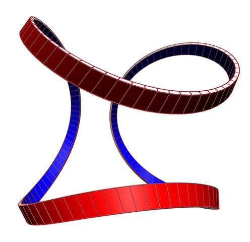
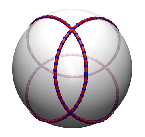
Figure 1: A force–free strip and the corresponding tangent curve.

In fact, there is a more elegant way to describe force–free strips without making use of the calculus of variation and differential equations we required for the previous arguments.
We will look at the tangent image $T$ of a Frenet curve $\gamma$ in $\mathbb{R}^{3}$ as a regular curve, i.e. as an equivalence class of parameterizations. Then there are many (not necessarily arclength parametrized) curves $\tilde{\gamma}$$\colon$$[0,\tilde{L}]\mapsto\mathbb{R}^{3}$ with the same tangent image $T$. We temporarily fix the tangent image and minimize $S_{-1}$ among all curves with the same tangent image.

Theorem .

Let $T$$\colon$$[0,\tilde{L}]\mapsto S^{2}$ be an arclength parametrized spherical curve with curvature $\lambda$. Then among all Frenet curves with tangent image $T$ the curve (54) minimizes $S_{-1}$ and is unique up to translations.

Proof.

For any curve $\tilde{\gamma}$ with tangent image $T$ and curvature $\tilde{\kappa}$ we have by the inequality between arithmetic and geometric mean

$$\begin{split}S_{-1}(\tilde{\gamma})&=\int_{0}^{\tilde{L}}(\tilde{\kappa}^{2}(1+\lambda^{2})^{2}+1)\frac{1}{\tilde{\kappa}}dt\\ &=\int_{0}^{\tilde{L}}(\tilde{\kappa}(1+\lambda^{2})^{2}+\frac{1}{\tilde{\kappa}})dt\\ &\geq\int_{0}^{\tilde{L}}2(1+\lambda^{2})dt\\ &=2L(\gamma)\\ &=S_{-1}(\gamma).\end{split}$$

∎

For force–free strips the bending energy is critical even if the end points of $\gamma$ are allowed to move, since the force vector $b_{0}$ comes from the boundary terms of the first variational formula. This implies that the boundary term drops out automatically. There are no conditions on the end points of $\gamma$ and the variational problem of $\gamma$ can be reduced to a variational problem on the tangent image. Consequently one can deduce Theorem 2 from the previous theorem, since $\int_{0}^{\tilde{L}}2(1+\lambda^{2})dt$ has a critical value iff $T$ is a spherical elastic curve with Lagrange multiplier 1. Langer and Singer [3] showed that there are infinitely many closed curves minimizing $\int_{0}^{\tilde{L}}2(1+\lambda^{2})dt$. Each such curve defines a closed force–free strip, since the mass center of $T$ is zero. In [References], it is shown that each closed spherical elastic curve with Lagrange multiplier 1 corresponds to a Willmore torus in $S^{3}$. More precisely, let $T$ be such a spherical curve, then we can parametrize all possible adapted frames (lifted to $S^{3}$) along the curve (54) by the frame cylinder $F:[0,\tilde{L}]\times S^{1}\rightarrow S^{3}$. $F$ is the preimage of the tangent image $T$ under the Hopf map $S^{3}\rightarrow S^{2}$ described in [References]. We obtain the following

Corollary.

The frame cylinder of a force–free strip is Willmore in $S^{3}.$

We generalize the previous method and reduce the variational problem to spherical curves.

Definition 4.

For an arclength parametrized spherical curve $T$ we call

$$P(T):=2\int_{0}^{\tilde{L}}\sqrt{\left\langle T,b_{0}\right\rangle-\mu}(1+\lambda^{2})ds$$ (61)

the P-functional.

Theorem .

For a critical point $\gamma$ of the modified Sadowsky functional the tangent vector $T$ with spherical curvature $\lambda$ is a critical point of the P-functional.

Proof.

Let $T$$\colon$$[0,\tilde{L}]\mapsto S^{2}$ be an arclength parametrized spherical curve with curvature $\lambda$. For any function $\kappa$$\colon$$[0,\tilde{L}]\mapsto\mathbb{R}^{+}$, we can define a regular space curve

$$\gamma(t)=\int_{0}^{{t}}\frac{1}{\kappa}Tds.$$ (62)

$\gamma$ has curvature $\kappa$ and the Sadowsky functional of $\gamma$ is given by

$$S(\kappa)=\int_{0}^{\tilde{L}}\kappa(1+\lambda^{2})^{2}ds.$$ (63)

We want to look for critical points of $S$ when $T$ is held fixed (only $\kappa$ varies). We do these variations of $\gamma$ under two constraints: The length

$$L=\int_{0}^{\tilde{L}}\frac{1}{\kappa}ds$$ (64)

and the end points of $\gamma$

$$\gamma(\tilde{L})=\int_{0}^{\tilde{L}}\frac{1}{\kappa}Tds$$ (65)

will be held fixed. These four scalar constraints allow us to add four Lagrange multipliers to the functional (63), conventionally gathered into a scalar $\mu$ and a vector $b_{0}\in\mathbb{R}^{3}$:

$$P_{T}(\kappa)=\int_{0}^{\tilde{L}}(\kappa(1+\lambda^{2})^{2}-\frac{\mu}{\kappa}+\frac{\left\langle T,b_{0}\right\rangle}{\kappa})ds.$$ (66)

Varying $\kappa$ yields

$$\dot{P}_{T}=\int_{0}^{\tilde{L}}(\dot{\kappa}((1+\lambda^{2})^{2}+\frac{\mu}{\kappa^{2}}-\frac{\left\langle T,b_{0}\right\rangle}{\kappa^{2}}))ds,$$ (67)

so $\kappa$ is critical for $P_{T}$ iff

$$\left\langle T,b_{0}\right\rangle=\kappa^{2}(1+\lambda^{2})^{2}+\mu.$$ (68)

Computing $\kappa$ from (68) yields

$$\kappa=\frac{\sqrt{\left\langle T,b_{0}\right\rangle-\mu}}{1+\lambda^{2}}.$$ (69)

Then $P_{T}$ becomes

$$P(T)=2\int_{0}^{\tilde{L}}\sqrt{\left\langle T,b_{0}\right\rangle-\mu}(1+\lambda^{2})ds.$$ (70)

This shows that for critical point $\gamma$ of $S_{\mu}$ the tangent image $T$ is a critical point of the P-functional. ∎

References

• [1] Th. Hangan, Elastic strips and differential geometry. Rend. Sem. Mat. Pol. Torino, 63, 2 (2005).
• [2] Th. Hangan, C. Murea, Elastic helices, Rev. Roumaine Mat. Pure App., 50 5-6 (2008), 641-645.
• [3] J. Langer, D. Singer, The total squared curvature of closed curves, J.Differential Geometry 20 (1984) 1-22.
• [4] U. Pinkall, Hopf tori in $S^{3}$. Invent. Math. 81. (1985), 379-386.
• [5] M. Romiger, Diplomarbeit zu elastischen Streifen, TU-Berlin, 2006.
• [6] M. Sadowsky, Ein elementarer Beweis f r die Existens eines abwickelbaren M biusschen Bandes und Zur ckf hrung des geometrischen Problems auf ein Variationsproblem. Sitzungsbericht Preussisch Akademischer Wissenschaften, 1930.
• [7] E.L. Starostin and G.H.M. van der Heijden, Natura Materials 6(8) (2007), 563-567.
• [8] E.L. Starostin and G.H.M. van der Heijden, Physical Review Letters 101, 084301 (2008).
• [9] E.L. Starostin and G.H.M. van der Heijden, Physical Review E 79, 066602 (2009).
• [10] W. Wunderlich, ber ein abwickelbares M biusband. (German)[J] Monatsh. Math. 66 (1962), 276-289 .