On internal wave breaking and tidal dissipation near the centre of a solar-type star

Abstract

We study the fate of internal gravity waves approaching the centre of an initially non-rotating solar-type star, primarily using two-dimensional numerical simulations based on a cylindrical model. A train of internal gravity waves is excited by tidal forcing at the interface between the convection and radiation zones of such a star. We derive a Boussinesq-type model of the central region of a star and find a nonlinear wave solution that is steady in the frame rotating with the angular pattern speed of the tidal forcing. We then use spectral methods to integrate the equations numerically, with the aim of studying at what amplitude the wave is subject to instabilities. These instabilities are found to lead to wave breaking whenever the amplitude exceeds a critical value. Below this critical value, the wave reflects perfectly from the centre of the star. Wave breaking leads to mean flow acceleration, which corresponds to a spin up of the central region of the star, and the formation of a critical layer, which acts as an absorbing barrier for subsequent ingoing waves. As these waves continue to be absorbed near the critical layer, the star is spun up from the inside out.

Our results point to an important amplitude dependence of the (modified) tidal quality factor $Q^{\prime}$, since nonlinear effects are responsible for dissipation at the centre of the star. If the amplitude of the tidal forcing exceeds the critical amplitude for wave breaking to occur, then this mechanism produces efficient dissipation over a continuous range of tidal frequencies. This requires $\left(\frac{m_{p}}{M_{J}}\right)\left(\frac{P}{1\;\mathrm{day}}\right)^{\frac{1}{6}}\gtrsim 3.3$, for a planet of mass $m_{p}$ in an orbit of period $P$ around the current Sun, neglecting stellar rotation. However, this criterion depends strongly on the strength of the stable stratification at the centre of the star, and so it depends on stellar mass and main-sequence age. If breaking occurs, we find $Q^{\prime}\approx 1.5\times 10^{5}\left(\frac{P}{1\;\mathrm{day}}\right)^{\frac{8}{3}}$, for the current Sun. This varies by no more than a factor of 5 throughout the range of solar-type stars with masses between $0.5-1.1M_{\odot}$, for fixed orbital parameters. This estimate of $Q^{\prime}$ is therefore quite robust, and can be reasonably considered to apply to all solar-type main-sequence stars, if this mechanism operates. The strong frequency dependence of the resulting dissipation means that this effect could be very important in determining the fate of close-in giant planets around G and K stars. We predict fewer giant planets with orbital periods of less than about 2 days around such stars if they cause breaking at the centre, due to the efficiency of this process.

Even if the waves are of too low amplitude to initiate breaking, radiative damping could, in principle, lead to a gradual spin-up of the stellar centre and to the formation of a critical layer. This process could provide efficient tidal dissipation in solar-type stars perturbed by less massive companions, but it may be prevented by effects that resist the development of differential rotation.

These mechanisms would, however, be ineffective in stars with a convective core, such as WASP-18, WASP-12 and OGLE-TR-56, perhaps partly explaining the survival of their close planetary companions.

1 Introduction

Tidal interactions are thought to be important in determining the fate of short-period extrasolar planets and the spins of their host stars, as well as in the sychronization and circularization of close binary stars. The extent of spin-orbit evolution that results from tides depends on the dissipative properties of the bodies involved in the interaction. It is standard to parametrize our uncertainties in the mechanisms of tidal dissipation in each body by defining a tidal quality factor $Q$, which is an inverse measure of the dissipation. This is usually defined to be proportional to the ratio of the maximum energy stored in a tidal oscillation ($E_{0}$) to the energy dissipated over one cycle, i.e.

$$Q=2\pi E_{0}\left(\oint-\dot{E}\,\mathrm{d}t\right)^{-1},$$ (1)

and we find it convenient to use the variant $Q^{\prime}=\frac{3Q}{2k}$, where $k$ is the second–order potential Love number of the body. This combination always appears together in the evolutionary equations.

$Q^{\prime}$ is difficult to calculate from first principles in fluid bodies, and uncertainties in the mechanisms of tidal dissipation remain. The tidal disturbance can generally be decomposed into two parts: an equilibrium tide and a dynamical tide. The equilibrium tide is the quasi-hydrostatic ellipsoidal tidal bulge. In the frame corotating with the fluid, the time-dependence of the equilibrium tide is dissipated through its interaction with turbulent convection, though the damping rate is uncertain, particularly when the convective time exceeds the tidal period (Zahn 1966; Goldreich & Nicholson 1977; Goodman & Oh 1997; Penev et al. 2007). The dynamical tide consists of internal waves that are excited by low-frequency tidal forcing, and has received much recent interest with regard to its possible contribution to $Q^{\prime}$ (Witte & Savonije 2002; Ogilvie & Lin 2004, hereafter OL04; Wu 2005; Papaloizou & Ivanov 2005; Ivanov & Papaloizou 2007; Ogilvie & Lin 2007, hereafter OL07; Goodman & Lackner 2009). This is because if these waves have short wavelength, then they are more easily damped than the large-scale equilibrium tide by radiative diffusion (Zahn 1975; Zahn 1977), convective viscosity (Terquem et al., 1998) or nonlinear breaking (Goodman & Dickson 1998; hereafter GD98).

The tidal frequency is typically much lower than the dynamical frequency of the body, so the relevant internal waves must be approximately incompressible, restored not by pressure but by buoyancy or rotation. OL04 found that the dissipation of tidally excited inertial waves, whose restoring force is the Coriolis force, can contribute significantly to the dissipation rate in a giant planet, whose interior is mostly convective (see also Wu 2005 and Ivanov & Papaloizou 2007). These waves can also contribute to the dissipation rate in convective regions of stars (OL07). They are excited by tidal forcing of frequency $\hat{\omega}$, if this is less than the Coriolis frequency ($2\Omega$), and this is true for many astrophysically relevant circumstances. However, these waves are not excited if the tidal frequency exceeds the Coriolis frequency, so this process is then not effective at dissipating the tide, and contributing to $Q^{\prime}$. In this work we concentrate on waves that have buoyancy as the restoring force, and which are commonly referred to as internal gravity waves (hereafter IGWs).

IGWs have been proposed to account for the efficient tidal dissipation that has been inferred from the circularisation of early-type binary stars (Zahn 1975; Zahn 1977; Zahn 2008; Savonije & Papaloizou 1983; Papaloizou & Savonije 1985; Savonije et al. 1995; Savonije & Papaloizou 1997; Papaloizou & Savonije 1997), which are massive enough to have a convective core and an exterior radiative envelope. In these stars, IGWs are excited near the boundary between these two regions, where the buoyancy frequency (or Brunt-Väisälä frequency, see § 2) matches the tidal forcing frequency. These propagate outwards into the stably stratified radiation zone, towards the surface, where they are fully or partially damped by radiative diffusion. In this picture, these stars are tidally synchronized from the outside in, since angular momentum is deposited in the regions of the star where these waves damp (Goldreich & Nicholson 1989a,b).

The above model only works for stars with an exterior radiation zone, which is unlike that of the Sun and other stars of solar type, which have radiative cores and convective envelopes. It is of particular interest to study the efficiency of tidal dissipation in these stars, since many have been found to harbour close-in planets, whose survival is determined by the stellar $Q^{\prime}$. This is because a planet with an orbital period shorter than the stellar spin period is subject to tidally induced orbital decay, with an inspiral time that depends on dissipation in the star (e.g. Barker & Ogilvie 2009; OL07) In these stars, a train of IGWs are again excited at the interface between the convective and radiative zones, but here they propagate towards the stellar centre. If they can coherently reflect from the centre, global standing modes can form in the radiation zone. In this case, tidal dissipation is efficient only when the tidal frequency matches that of a global standing mode (which are commonly referred to as $g$-modes) (Terquem et al. 1998; Savonije & Witte 2002). This would not contribute appreciably to $Q^{\prime}$ because the system would evolve rapidly through these resonances, unless resonance locking occurs (Witte & Savonije 1999; Witte & Savonije 2001). On the other hand, if these waves do not reflect coherently from the centre, and are either strongly dissipated there, or are reflected with a perturbed phase, then efficient dissipation is possible over a broad range of tidal frequencies (GD98; OL07). The extent of nonlinearity in the waves near the centre is likely to be the factor that determines whether these waves reflect coherently, and this is controlled by the amplitude and frequency of the tidal forcing, as well as the properties of the stellar centre (OL07).

In this paper we study the problem of IGWs approaching the centre of a solar-type star, primarily using two-dimensional numerical simulations. We first derive a Boussinesq-type system of equations appropriate for the stellar centre, which are ideal for integrating numerically using spectral methods. An exact solution for tidally forced waves is derived, and some of its properties are discussed. Our numerical set-up is described and results are presented for both linear and nonlinear forcing amplitudes, including an analysis of the reflection coefficient and a study of the growth of different azimuthal wavenumbers in the disturbance. This is followed by a discussion of the results, especially their relevance to $Q^{\prime}$ for solar-type stars, and to the survival of close-in giant planets in orbit around such stars.

2 Internal gravity waves: elementary properties, wave breaking and critical layers

IGWs are a family of dispersive waves that are ubiquitous in nature. They propagate in any fluid with a stable density stratification, due to the restoring force of buoyancy. Their influence can be observed in the oceans and atmosphere of the Earth on a range of spatial and temporal scales, from the visual undulations of striated cloud structures, to the complex interplay between these waves and shearing flows, which produces the large-scale Quasi-Biennial Oscillation in the equatorial stratosphere. It is widely recognised that IGWs play a prominent role in the transport of energy and angular momentum in geophysical and astrophysical flows (Bühler 2009; McIntyre 2000; Rogers & Glatzmaier 2006; Kumar et al. 1999). IGWs are also thought to be important in stably stratified radiation zones of stars. When excited by turbulent convection, they were at one stage put forward as potential explanations for maintaining the solid body rotation of the radiative interior of the Sun (Schatzman 1993; Zahn et al. 1997). However, it was pointed out that the “antidiffusive” nature of IGWs tends to enhance local shear rather than reduce it (Gough & McIntyre, 1998). IGWs are still thought to produce angular velocity variations in the radiation zone (Rogers & Glatzmaier, 2006). They have also been invoked to explain the Li depletion problem in F-stars (Garcia Lopez & Spruit, 1991), affecting solar neutrino production (Press, 1981), and possibly having an effect on the solar cycle (Kumar et al., 1999).

Observations of oscillations on the solar surface are able to provide information about the interior properties of the Sun (Christensen-Dalsgaard, 2002). IGWs in the radiative interior of the Sun can form global standing modes, commonly referred to as $g$-modes, if their frequency matches that of a free mode of oscillation. These are known to have their amplitude largest close to the centre (see solution in § 5) and would therefore seem ideal probes of the deep interior. Unfortunately for observers, the standing $g$-modes are effectively trapped in the radiative interior, where the stratification is stable, and are evanescent in the convection zone, and so are unlikely to be visible at the solar surface. Nevertheless, modes of sufficiently low degree, with high enough amplitude, may have already been observed at the surface by García et al. (2007), though it must be noted that thus far there is no undisputed evidence for observations of $g$-modes (Appourchaux et al., 2009).

The frequencies of the largely incompressible internal waves lie in ranges controlled by the buoyancy frequency (or Brunt-Väisälä frequency) $N$ and the Coriolis frequency $2\Omega$. The square of the buoyancy frequency in a spherically symmetric star is defined by

$$N^{2}(r)=-\frac{1}{\rho}\frac{dp}{dr}\left(\frac{1}{\Gamma_{1}}\frac{d\ln p}{dr}-\frac{d\ln\rho}{dr}\right),$$ (2)

where $\rho,p$ are the density and pressure, and $\Gamma_{1}=\left(\frac{\partial\ln p}{\partial\ln\rho}\right)_{s}$ (at constant specific entropy $s$). The local dispersion relation for linear noncompressive internal waves in a fluid body rotating with angular velocity $\mathbf{\Omega}$ is

$$\omega^{2}=N^{2}\sin^{2}\alpha+4\Omega^{2}\cos^{2}\beta,$$ (3)

where $\alpha$ is the angle between the wavevector $\mathbf{k}$ and the gravitational acceleration $\mathbf{g}$, and $\beta$ is the angle between $\mathbf{k}$ and $\mathbf{\Omega}$. The frequency of these waves is independent of wavelength (in the absence of viscosity or thermal conduction), and only depends on the direction of the wavevector. This is different from waves whose restoring force is due to compressibility, whose frequency is inversely proportional to wavelength. When $N=0$, Eq.4 describes inertial waves, which have frequencies in the range $(0,2\Omega)$. If the body is non-rotating ($\mathbf{\Omega}=0$), then these waves are IGWs, and possess frequencies in the range $(0,N)$. In the presence of nonzero $\mathbf{\Omega}$ and $N$, these waves are intermediate between inertial waves and IGWs and are referred to as inertia-gravity waves. For waves in a spherical star, at a given latitude there is a minimum frequency for inertia-gravity wave propagation. Near the equator, waves can propagate with arbitrarily low frequency. From here on we neglect the bulk rotation, and assume that $\mathbf{\Omega}=0$, i.e., we consider only IGWs. The local dispersion relation for IGWs can be rewritten

$$\omega^{2}=N^{2}\frac{k^{2}_{h}}{k^{2}_{r}+k^{2}_{h}},$$ (4)

where $k_{h}$ and $k_{r}$ are the horizontal and radial wavenumbers.

The phase and group velocities of these waves can be calculated from Eq. 4 to give

$$\mathbf{c}_{p} = \frac{\omega}{|\mathbf{k}|}\frac{\mathbf{k}}{|\mathbf{k}|}=\frac{Nk_{h}}{(k^{2}_{r}+k^{2}_{h})^{\frac{3}{2}}}\left(k_{r}\mathbf{e}_{r}+k_{h}\mathbf{e}_{h}\right)$$ (5)

$$\approx \frac{Nk_{h}}{k^{3}_{r}}\left(k_{r}\mathbf{e}_{r}+k_{h}\mathbf{e}_{h}\right)$$ (6)

$$\mathbf{c}_{g} = \nabla_{\mathbf{k}}\omega=-\frac{Nk_{r}}{(k^{2}_{r}+k^{2}_{h})^{\frac{3}{2}}}\left(k_{h}\mathbf{e}_{r}-k_{r}\mathbf{e}_{h}\right)$$ (7)

$$\approx -\frac{N}{k_{r}^{2}}\left(k_{h}\mathbf{e}_{r}-k_{r}\mathbf{e}_{h}\right),$$ (8)

in the tidally relevant limit that the radial wavelength of the waves is much shorter than the horizontal wavelength, i.e., $k_{h}\ll k_{r}$ (which is true except near turning points or within the last few wavelengths from the centre of a star). In this limit, $\mathbf{c}_{g}\cdot\mathbf{e}_{r}=-N\frac{k_{h}}{k_{r}^{2}}=-\mathbf{c}_{p}\cdot\mathbf{e}_{r}$, i.e., the radial wave pattern moves in the opposite direction to the radial energy flux. Since $\omega$ is independent of $|\mathbf{k}|$, $\mathbf{c}_{g}\cdot\mathbf{k}=0$, meaning that the energy in IGWs propagates along surfaces of constant phase.

For waves on a non-zero horizontal background shear flow $\mathbf{U}$, Eq. 4 still applies if the Richardson number $Ri=\frac{N^{2}}{|\partial\mathbf{U}/\partial r|^{2}}\gg 1$, if we replace $\omega$ by the Doppler-shifted frequency $\hat{\omega}$, and similarly for the phase and group velocity of the waves

$$\hat{\omega}=\omega-\mathbf{k}\cdot\mathbf{U},\;\;\;\;\hat{\mathbf{c}}_{p}=\mathbf{c}_{p}-\mathbf{U},\;\;\;\;\hat{\mathbf{c}}_{g}=\mathbf{c}_{g}-\mathbf{U}.$$ (9)

We now have the possibility of the wave frequency being Doppler-shifted upwards to $N$, in which case $\hat{\mathbf{c}}_{g}\cdot\mathbf{e}_{r}$ reverses, giving total internal reflection (McIntyre, 2000).

The other extreme, that $\hat{\omega}\rightarrow 0$, occurs when the horizontal velocity in the shear matches that of the horizontal phase velocity. This occurs at a so-called critical layer, which is defined as the layer at which the wavelength of the waves would be Doppler-shifted to zero, if they were ever to reach it. Note though, that $\hat{\mathbf{c}}_{g}\cdot\mathbf{e}_{r}\rightarrow 0$ as $\hat{\omega}\rightarrow 0$, so in linear theory the waves never reach the critical layer in a finite time. Early work on IGWs in a background shear, including a study of critical layers, can be found in Booker & Bretherton (1967) and Hazel (1967). They find that an IGW propagating through a critical layer is attenuated by a factor $\sim\exp\left(-2\pi(Ri-1/4)^{1/2}\right)$. If $Ri\gg 1/4$, the wave is fully absorbed, and irreversibly transfers its energy to the mean flow. However, it must be noted that at the critical layer, linear theory predicts that the wave steepness

$$s=\frac{\mathrm{max}(\mathbf{u}\cdot\mathbf{e}_{h})}{\hat{\mathbf{c}}_{p}\cdot\mathbf{e}_{h}},$$ (10)

where $\mathbf{u}$ is the velocity perturbation, of these waves goes to infinity, as the Doppler-shifted horizontal phase speed $\hat{\mathbf{c}}_{p}\cdot\mathbf{e}_{h}$ goes to zero, i.e., the waves become strongly nonlinear at the critical layer (which McIntyre 2000 refers to as linear theory predicting its own breakdown). Since wave breaking is expected to occur whenever $s>1$, the waves are likely to break before they reach the critical layer. Nonlinear effects have been studied in early simulations by Winters & D’Asaro (1994), who find that the of initial wave energy on encountering a critical layer, roughly one third reflects, one third results in mean flow acceleration and the remainder cascades to small scales where it is dissipated. This implies that wave absorption by the mean flow need not be complete, in contrast with the prediction from linear theory. This is discussed further in § 9.2 in relation to the results of our simulations.

Wave breaking is defined as a wave-induced process that leads to the rapid and irreversible deformation of otherwise wavy material contours (McIntyre, 2000), and it leads to the production of turbulence and irreversible energy dissipation. The breaking process results from the growth of an instability upon a basic state composed of a wave with $s>1$. The susceptibility of a wave to breaking can be enhanced by resonant triad interactions, in which a primary wave resonantly interacts with a pair of low-amplitude secondary waves. This process transfers energy to the secondary waves, whose steepness can then grow beyond the critical value required for breaking to occur, even though the primary steepness may not be sufficient for breaking on its own (Staquet & Sommeria, 2002). Previous work has shown that the process leading to the wave steepening is two-dimensional, but that breaking is a three-dimensional process (Klostermeyer 1991;Winters & D’Asaro 1994). Nevertheless, the mechanisms responsible for breaking and the final outcome of the breaking process are likely to be similar in 2D.

Here we are interested in studying what happens when IGWs excited by tidal forcing approach the centre of a star with an inner radiation zone, i.e. G-type stars such as the Sun, which do not possess a convective core. We are primarily concerned with the tidal dissipation efficiency for solar-type stars that may result from breaking of these waves near the centre. Throughout the rest of this paper we restrict our problem to 2D, and postpone study of any 3D effects. We now describe our basic problem in more detail.

3 Basic description of the problem

3.1 Tidal potential

Consider a star and a planet in a mutual Keplerian orbit (though we make no assumptions about the relative masses at this stage). The tidal potential experienced by the star can be written as a sum of rigidly rotating spherical harmonics (e.g. OL04). For the simplest case of a planet on a circular orbit, that is coplanar with the equatorial plane of the star, we can consider a two-dimensional restriction of the problem to this plane. This allows us to write the time-dependent part of the quadrupolar ($l=2$) tidal potential in the equatorial plane of the star as

$$\Psi(r,\phi,t)=-\frac{3}{4}\frac{Gm_{p}}{a^{3}}r^{2}\cos(2\phi-\hat{\omega}t),$$ (11)

in spherical polar coordinates $(r,\theta,\phi)$ with origin at the centre of the star, in the plane $\theta=\pi/2$. Here $m_{p}$ is the planet mass, $a$ is the orbital semi-major axis, and $n>0$ is the mean motion. The relevant tidal frequency is $\hat{\omega}=2n-2\Omega$ for a star rotating with angular velocity $\Omega$. From here on we assume that the star is non-rotating, i.e. we assume that $\Omega=0$, which is a reasonable assumption if the star is spinning much slower than the orbit. This is justified for the problem of a close-in gas giant planet with a several-day orbital period around a solar-type star that has been spun down by magnetic braking for the duration that it has spent on the main sequence, to rotate with a spin period of several tens of days.

We consider a restriction of the full three-dimensional problem, in which the tidal potential is composed of many different spherical harmonic components for an orbit of arbitrary eccentricity and inclination, to instead consider a simplified two dimensional model of a star, forced by this single component of the tide. The main motivation for this decision is simplicity, since this is a first attack on the problem, though it is likely that this is a reasonable approximation. Extensions can be studied in the future.

3.2 Central regions of a star

The buoyancy frequency is real and comparable with the dynamical frequency of the star

$$\omega_{dyn}=\left(\frac{Gm_{\star}}{R_{\star}^{3}}\right)^{\frac{1}{2}},$$ (12)

throughout the bulk of the radiation zone, where $m_{\star}$ and $R_{\star}$ are the stellar mass and radius, respectively. In Fig. 1 we plot $N$ normalised to $\omega_{dyn}$ in the radiation zone for Model S of the current Sun (Christensen-Dalsgaard et al., 1996). For our problem, the tidal frequencies of interest $\hat{\omega}\ll N$, which implies $k_{r}\gg 2\pi/r$, except near the centre. IGWs are excited at the top of the radiation zone by a combination of tidal forcing in that region, together with the pressure of inertial waves acting at the interface if $|\hat{\omega}|<2\Omega$ (OL07). It is within this transition region that $N$ increases linearly with distance into the radiation zone, so there is a point at which $N\sim\hat{\omega}$, and IGWs are efficiently excited. These propagate towards the centre with radial wavelengths $\lambda_{r}\lesssim 10^{-3}-10^{-2}R_{\odot}$, for typical tidal frequencies.

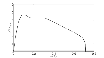
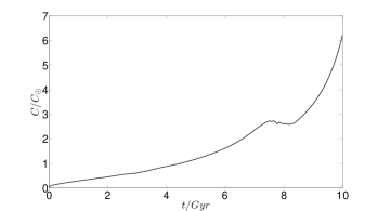
Figure 1: Top: Buoyancy frequency $N$ normalised to dynamical frequency $\omega_{dyn}$ versus radius, based on Model S of the current Sun. Also plotted is a frequency $2\pi/1\mathrm{day}\sim 0.1\omega_{dyn}$, corresponding with the orbital frequency for a one day orbit – note that this is half the tidal frequency, so $\hat{\omega}\ll N$ throughout the bulk of the radiation zone. Only near the centre and at the interface between the convection and radiation zones, does $\hat{\omega}\sim N$. Bottom: Coefficient $C$ in the expansion $N\approx Cr$ near the centre of the Sun normalised to its current value versus main-sequence age for a sequence of solar models that pass through Model S of the current Sun. The stratification steepens as the star evolves.

Expanding the standard equations of stellar structure about $r=0$, we obtain the density stratification

$$\rho(r)=\rho_{0}+\rho_{2}r^{2}+O(r^{4}).$$ (13)

For sufficiently small $r$, $g$ is linear in $r$, and $N=Cr$ is also linear in $r$, where $C$ is a constant that varies with stellar model and main-sequence age. For the current Sun, $C\equiv C_{\odot}\approx 8.0\times 10^{-11}\mathrm{m}^{-1}\mathrm{s}^{-1}$. This is valid throughout only the inner $\lesssim 3\%$ of the Sun. However, even with the largest expected radial wavelength, this region contains multiple wavelengths. In Fig. 1 we plot the variation in $C$ versus main-sequence age, normalised to its value in the current Sun, from a sequence of solar models that pass through Model S. The increase in $C$ with age is due both to the increasing central condensation, and the build-up of a gradient in the hydrogen abundance (there is a small drop around $8$ Gyr when hydrogen is nearly used up and the contribution from the composition gradient decreases, after which the central density increases rapidly).

4 Derivation of a Boussinesq-type system of equations

The ideal compressible fluid equations in 2D plane polar ($r,\phi$) coordinates are

$$Du_{r}-\frac{u_{\phi}^{2}}{r}=-\frac{1}{\rho}\partial_{r}p-\partial_{r}\Phi,$$ (14)

$$Du_{\phi}+\frac{u_{r}u_{\phi}}{r}=-\frac{1}{\rho r}\partial_{\phi}p-\frac{1}{r}\partial_{\phi}\Phi,$$ (15)

$$D\rho+\rho\left[\frac{1}{r}\partial_{r}(ru_{r})+\frac{1}{r}\partial_{\phi}u_{\phi}\right]=0,$$ (16)

$$Dp-\frac{\gamma p}{\rho}D\rho=0,$$ (17)

$$D=\partial_{t}+u_{r}\partial_{r}+\frac{u_{\phi}}{r}\partial_{\phi},$$ (18)

$$\nabla^{2}\Phi=4\pi G\rho.$$ (19)

The basic state is static and circularly symmetric. Near the centre, we pose the expansion

$$\rho=\rho_{0}+\rho_{2}r^{2}+\rho_{4}r^{4}+O(r^{6}),$$ (20)

and similarly for $p$ and $\Phi$. The coefficients are related by the condition for the background to be in hydrostatic equilibrium, together with Poisson’s equation, giving

$$p_{2}=-\rho_{0}\Phi_{2},\;\;p_{4}=-\rho_{0}\Phi_{4}+\frac{p_{2}\rho_{2}}{2\rho_{0}},$$ (21)

$$\Phi_{2}=\pi G\rho_{0},\;\;\Phi_{4}=\frac{\pi G\rho_{2}}{4},$$ (22)

and so on for the coefficients of higher-order terms.

We are interested in a region where $r/R_{\star}=O(\epsilon)$, where $\epsilon\ll 1$, so let $r=\epsilon x$. Now introduce a slow time $\tau=\epsilon t$, then the solution including the basic state and a slow nonlinear density perturbation has the form

$$\rho=\underbrace{\rho_{0}+\epsilon^{2}\rho_{2}x^{2}+\epsilon^{4}\rho_{4}x^{4}+...}_{\mathrm{basic\;state}}+\underbrace{\epsilon^{2}\rho^{\prime}_{2}(x,\phi,\tau)+...}_{\mathrm{nonlinear\;perturbation}},$$ (23)

$$p=\underbrace{p_{0}+\epsilon^{2}p_{2}x^{2}+\epsilon^{4}p_{4}x^{4}+...}_{\mathrm{basic\;state}}+\underbrace{\epsilon^{4}p^{\prime}_{4}(x,\phi,\tau)+...}_{\mathrm{nonlinear\;perturbation}},$$ (24)

$$\Phi=\underbrace{\Phi_{0}+\epsilon^{2}\Phi_{2}x^{2}+\epsilon^{4}\Phi_{4}x^{4}+...}_{\mathrm{basic\;state}}+\underbrace{\epsilon^{4}\Phi^{\prime}_{4}(x,\phi,\tau)+...}_{\mathrm{nonlinear\;perturbation}},$$ (25)

$$u_{r}=\underbrace{\epsilon^{2}u_{r2}(x,\phi,\tau)+...}_{\mathrm{nonlinear\;perturbation}},$$ (26)

$$u_{\phi}=\underbrace{\epsilon^{2}u_{\phi 2}(x,\phi,\tau)+...}_{\mathrm{nonlinear\;perturbation}},$$ (27)

In the Boussinesq approximation, the fractional pressure perturbation is small compared with the fractional density perturbation because this is a low-frequency perturbation, with $\omega\ll\omega_{dyn}$, for which acoustic effects are negligible. For such short-wavelength perturbations, the gravitational perturbation is also small (Christensen-Dalsgaard, 2002). These two points explain the absence of terms in the above solutions proportional to $\epsilon^{2}$ for $p$ and $\Phi$ in the nonlinear perturbation. This corresponds to looking for small density constrasts and weak material accelerations compared with gravity.

Substituting these expansions into the basic equations, and subtracting terms that arise only in the basic state, we obtain at leading order

$$D_{1}u_{r2}-\frac{u_{\phi 2}^{2}}{x}=-\frac{1}{\rho_{0}}\partial_{x}p^{\prime}_{4}+\frac{2xp_{2}\rho_{2}^{\prime}}{\rho_{0}^{2}}-\partial_{x}\Phi^{\prime}_{4},$$ (28)

$$D_{1}u_{\phi 2}+\frac{u_{r2}u_{\phi 2}}{x}=-\frac{1}{\rho_{0}x}\partial_{\phi}p^{\prime}_{4}-\frac{1}{x}\partial_{\phi}\Phi^{\prime}_{4},$$ (29)

$$\rho_{0}\left[\frac{1}{x}\partial_{x}(xu_{r2})+\frac{1}{x}\partial_{\phi}u_{\phi 2}\right]=0,$$ (30)

$$2xp_{2}u_{r2}-\frac{\gamma p_{0}}{\rho_{0}}\left(D_{1}\rho^{\prime}_{2}+2x\rho_{2}u_{r2}\right)=0,$$ (31)

$$D_{1}=\partial_{\tau}+u_{r2}\partial_{x}+\frac{u_{\phi 2}}{x}\partial_{\phi},$$ (32)

$$\nabla^{2}\Phi^{\prime}_{4}=4\pi G\rho_{2}^{\prime}.$$ (33)

Note that Poisson’s equation is no longer required, since we have separated out the gravitational potential perturbation in this approximation, which is equivalent to Cowling’s approximation (Cowling, 1941).

We can rewrite these equations in a more natural notation, removing the asymptotic scalings to find

$$Du_{r}-\frac{u_{\phi}^{2}}{r}=-\partial_{r}q+rb,$$ (34)

$$Du_{\phi}+\frac{u_{r}u_{\phi}}{r}=-\frac{1}{\rho r}\partial_{\phi}q,$$ (35)

$$\frac{1}{r}\partial_{r}(ru_{r})+\frac{1}{r}\partial_{\phi}u_{\phi}=0,$$ (36)

$$Db+C^{2}ru_{r}=0,$$ (37)

$$D=\partial_{t}+u_{r}\partial_{r}+\frac{u_{\phi}}{r}\partial_{\phi},$$ (38)

where

$$b=\frac{2p_{2}}{\rho_{0}^{2}}\rho^{\prime}_{2},$$ (39)

$$q=\frac{1}{\rho_{0}}p_{4}^{\prime}+\Phi_{4}^{\prime},$$ (40)

are a buoyancy variable and a modified pressure variable, and

$$C^{2}=4\Phi_{2}\left(\frac{p_{2}}{\gamma p_{0}}-\frac{\rho_{2}}{\rho_{0}}\right)$$ (41)

is related to the buoyancy frequency $N$ by $N=Cr$, with $C^{2}>0$ for a stably stratified centre of a star.

We now write them in the vector-invariant form

$$D\mathbf{u}=-\nabla q+\mathbf{r}b,$$ (43)

$$Db+C^{2}\mathbf{r}\cdot\mathbf{u}=0,$$

$$\nabla\cdot\mathbf{u}=0,$$ (44)

$$D=\partial_{t}+\mathbf{u}\cdot\nabla.$$ (45)

These equations are similar to the standard Boussinesq system for a slab of fluid in Cartesian geometry (see e.g. Bühler 2009, Ch. 6) with a uniform stratification, with the exception that our problem is in cylindrical geometry, with $g$ and $N$ proportional to $r$. Note also that the buoyancy variable defined here is related, but not identical, to that of the standard Boussinesq approximation used in atmospheric sciences and oceanography (see e.g. Bühler 2009). The buoyancy variable is proportional to the density and entropy perturbation.

An energy equation for our system can be derived by contracting Eq. 43 with $\mathbf{u}$:

$$\partial_{t}\left(\frac{1}{2}|\mathbf{u}|^{2}+\frac{b^{2}}{2C^{2}}\right)+\nabla\cdot\left[\left(\frac{1}{2}|\mathbf{u}|^{2}+\frac{b^{2}}{2C^{2}}+q\right)\mathbf{u}\right]=0.$$ (46)

Thus $E=\frac{1}{2}\rho_{0}|\mathbf{u}|^{2}+\rho_{0}\frac{b^{2}}{2C^{2}}$ is the energy density per unit volume, and $\mathbf{F}_{E}=\rho_{0}\left(\frac{1}{2}|\mathbf{u}|^{2}+\frac{b^{2}}{2C^{2}}+q\right)\mathbf{u}$ is the energy flux density.

If the fluid is at rest, with $b=0$, then the stratification surfaces are circles (spheres in 3D), and $C^{2}$ measures the strength of the stable stratification. If we disturb the fluid from rest, then a positive (negative) buoyancy is associated with an inward (outward) radial displacement of particles, resulting in an outward (inward) acceleration of the fluid due to buoyancy to restore the system to equilibrium. From the energy equation Eq. 46, we can see that the state $b=0$ is the state of minimum gravitational potential energy, since the available potential energy density $\rho_{0}\frac{b^{2}}{2C^{2}}$ is minimised for this state. This makes sense, since this corresponds to having a background state with no wave-like disturbance.

5 Linear theory of IGWs approaching the stellar centre

5.1 Linear solution steady in a frame rotating with the pattern speed of forcing

If the radiation zone is forced from above then this will excite waves, which will propagate to the centre of the star. If the incoming wave has frequency $\omega$ and azimuthal wavenumber $m$, then it seems reasonable to assume that the response is steady in a frame rotating with the angular pattern speed of the forcing $\Omega_{p}=\omega/m$, in the absence of instabilities. The dependence on $\phi$ and $t$ is then only through the combination

$$\xi=m\phi-\omega t=m(\phi-\Omega_{p}t).$$ (47)

We can choose $\Omega_{p}/C$ as a unit of length, and $\Omega_{p}^{-1}$ as a unit of time (note that these units are only used in this section and in Appendix A), to allow us to write the equations in the dimensionless form

$$Du_{r}-\frac{u_{\phi}^{2}}{r}=-\partial_{r}q+rb,$$ (48)

$$Du_{\phi}+\frac{u_{r}u_{\phi}}{r}=-\frac{m}{\rho r}\partial_{\xi}q,$$ (49)

$$\frac{1}{r}\partial_{r}(ru_{r})+\frac{m}{r}\partial_{\xi}u_{\phi},$$ (50)

$$Db+ru_{r}=0,$$ (51)

$$D=u_{r}\partial_{r}+m\left(\frac{u_{\phi}}{r}-1\right)\partial_{\xi}.$$ (52)

The energy equation (Eq. 46) allows us to infer that the radial energy flux

$$F^{E}_{r}=\rho_{0}\int_{0}^{2\pi}\left[\frac{1}{2}\left(|\mathbf{u}|^{2}+b^{2}\right)+q\right]ru_{r}d\xi$$ (53)

is independent of $r$ for disturbances steady in this frame of reference, since the solutions are periodic with period $2\pi$ starting at $\xi=0$.

The radial angular momentum flux is

$$F^{L}_{r}=\frac{m}{\omega}F^{E}_{r}.$$ (54)

We can obtain a solution to these equations by linearization as follows, assuming that the solution is proportional to $e^{i\xi}$. Then we obtain (where real parts are assumed to be taken)

$$-imu_{r}=-\partial_{r}q+rb,$$ (55)

$$-imu_{\phi}=-\frac{imq}{r},$$ (56)

$$\frac{1}{r}\partial_{r}(ru_{r})+\frac{im}{r}u_{\phi}=0,$$ (57)

$$-imb+ru_{r}=0.$$ (58)

The incompressibility constraint allows us to express the velocity in terms of the streamfunction $\psi(r,\phi)$, which is defined by

$$\mathbf{u}=\nabla\times\left(\psi\mathbf{e}_{z}\right)=\left(\frac{1}{r}\partial_{\phi}\psi\right)\mathbf{e}_{r}+\left(-\partial_{r}\psi\right)\mathbf{e}_{\phi},$$ (59)

so we can write

$$u_{r}=\mathrm{Re}\left[\frac{im}{r}\psi\right],$$ (60)

$$u_{\phi}=\mathrm{Re}\left[-\partial_{r}\psi\right].$$ (61)

This enables us to reduce the system to Bessel’s equation of order $m$,

$$L_{m}\psi=\partial_{r}(r\partial_{r}\psi)+r\left(1-\frac{m^{2}}{r^{2}}\right)\psi=0$$ (62)

with solution regular at the origin $\psi\propto J_{m}(r)$. This represents a wave that approaches from infinity, reflects perfectly from the centre and goes out to infinity. Pure ingoing and outgoing wave solutions are described by $J_{m}(r)\pm iY_{m}(r)$ respectively.

5.2 Properties of the (non-)linear solution

The general solution can be written in the form of a sum of ingoing and outgoing waves, with complex amplitudes $A_{in}$ and $A_{out}$, as follows:

$$\psi_{in}(r,\xi)=[J_{m}(r)+iY_{m}(r)]e^{i\xi},$$ (63)

$$\psi_{out}(r,\xi)=[J_{m}(r)-iY_{m}(r)]e^{i\xi},$$ (64)

$$\psi(r,\xi)=A_{in}\psi_{in}(r,\xi)+A_{out}\psi_{out}(r,\xi).$$ (65)

We can check that $\psi_{in}$ corresponds to an ingoing wave by calculating its phase and group velocities. A simple calculation shows that the radial phase velocity is directed outward if we adopt the convention that $\omega=m\Omega_{p}>0$, and the group velocity is directed inward. This highlights one of the peculiarities of IGWs – that the phase and group velocities are oppositely directed, as discussed in § 2. For these linear waves, we have

$$F^{E}_{r}=\rho_{0}\pi mr\mathrm{Im}[\psi\partial_{r}\psi^{*}]=2m\rho_{0}\left(|A_{out}|^{2}-|A_{in}|^{2}\right).$$ (66)

The solution for a wave that perfectly reflects from the centre is

$$\psi(r,\xi)=2A_{in}J_{m}(r)e^{i\xi},$$ (67)

and has $F^{E}_{r}=0$, since $A_{in}=A_{out}$.

If we take the curl of Eq. 43, we obtain

$$\partial_{t}(\nabla\times\mathbf{u})=\nabla\times(\mathbf{r}b)-\nabla\times(\mathbf{u}\cdot\nabla\mathbf{u}),$$ (68)

which has eliminated the modified pressure perturbation $q$. The $z$-component of this equation expressed in terms of the streamfunction is

$$\partial_{t}(-\nabla^{2}\psi)=-\partial_{\phi}b+J(\psi,-\nabla^{2}\psi),$$ (69)

and the buoyancy equation is

$$\partial_{t}b=-C^{2}\partial_{\phi}\psi+J(\psi,b).$$ (70)

The nonlinear terms take the form of Jacobians,

$$J(A,B) = \frac{\partial(A,B)}{\partial(x,y)}=\frac{1}{r}\frac{\partial(A,B)}{\partial(r,\phi)}$$ (71)

$$= (\partial_{r}A)(\frac{1}{r}\partial_{\phi}B)-(\frac{1}{r}\partial_{\phi}A)(\partial_{r}B).$$ (72)

The Jacobians of the solution derived above are

$$J(\psi,-\nabla^{2}\psi)=J(\psi,b)=0,$$ (73)

which expresses the surprising result that the solutions derived are exact nonlinear solutions of the system. This follows from the fact that $-\nabla^{2}\psi=b=\psi$ for these waves. This arises because although the nonlinear terms $\mathbf{u}\cdot\nabla\mathbf{u}\neq 0$, they are balanced by the modified pressure term in the equations of motion. We also have $\mathbf{u}\cdot\nabla b=0$.

This is distinct from, but analogous to, the result that a single propagating plane IGW in a uniform stratification is a nonlinear solution of the standard Boussinesq system (Drazin 1977; Klostermeyer 1982). This is a consequence of the fact that $\mathbf{k}\cdot\mathbf{u}=0$ for these waves, which implies that the advective operator $\mathbf{u}\cdot\nabla$ annihilates any disturbance belonging to the same plane wave. A useful consequence of this is that a stability analysis can be performed on finite-amplitude propagating IGWs, allowing detailed understanding of the initial stages of the breaking process for these waves (Drazin 1977; Klostermeyer 1982; Klostermeyer 1991). Such studies have shown that a single propagating IGW solution is always unstable whatever its amplitude, since it undergoes resonant triad interactions (Drazin, 1977). One important difference in our problem is that the nonlinearity is spatially localized to the innermost wavelengths, whereas the nonlinearity is present everywhere in the plane IGW problem. We postpone a study of the stability of our nonlinear standing wave until a subsequent paper, though we expect waves of sufficiently large amplitude to be unstable if they overturn the stratification.

The amplitude required to overturn the stratification can be derived from our solution Eq. 67. The entropy (or more precisely, a quantity proportional to the entropy) is $s=b+(1/2)r^{2}$, in these units. Overturning the stratification means that the entropy profile, perturbed by a wave with buoyancy perturbation $b$, must satisfy $\partial_{r}s<0$, which implies $(1/r)\partial_{r}b<-1$ is a condition for overturning. Since $b=\psi$ for these nonlinear waves, this can be expressed in terms of the streamfunction as $(1/r)\partial_{r}\psi<-1$. Reintroducing dimensional variables, and substituting for $u_{\phi}$, modifies this criterion to $(u_{\phi}/r)>\Omega_{p}$, i.e., overturning occurs if the angular velocity of the wave exceeds the angular pattern speed. Equivalently, wave breaking occurs if

$$\mathrm{max}(u_{\phi})\gtrsim\frac{\omega^{2}}{4C},$$ (74)

whose largest value occurs where the amplitude of $\partial_{r}J_{2}(r)$ is largest, which is one wavelength from the centre.

In 3D the equivalent linear solution (written down in the Appendix of OL07), is not an exact nonlinear solution. However, the results of a weakly nonlinear analysis find that the reflection is close to perfect, with a reflection coefficient that is extremely close to unity for moderate amplitudes.

6 Numerical methods

6.1 Snoopy spectral code

We solve the system of equations (43)-(45) using a Cartesian spectral code, Snoopy (Lesur & Longaretti 2005; Lesur & Longaretti 2007). It is advantageous to use a Cartesian code over one in the more natural (for the problem) cylindrical geometry, because of the absence of a coordinate singularity at the origin, near to which is the region of the flow that we are most interested in. We also avoid the timestep issues close to the centre that would be present in a time-explicit cylindrical code. These arise from the CFL condition, because the grid spacing becomes very small near the origin.

Since this is a Fourier spectral code, the problem must be periodic in space. We solve our non-periodic problem using this code by setting up a region near the outer boundary, in which the fluid variables are smoothed to zero as we approach the boundary, using a parabolic smoothing function. We find it is quite acceptable to do this over a region about $1/10$ of the total box size. For this value there is negligible interaction between neighbouring boxes. This approach is one that may be useful in many applications which would benefit from the use of spectral methods, but have non-cartesian geometry and/or non-periodic boundary conditions. The obvious drawback of such an approach is the slight increase in computational cost, since the smoothing region is additional to the flow in the region of interest. Interior to this we have a thin ring in which we implement a forcing term in the radial momentum equation of the form $f_{r}\cos(2\phi-\omega t)$. This is designed to excite IGWs with $m=2$, but is not designed to accurately describe the excitation of IGWs at the top of the radiation zone, since we are only interested in the dynamics of the central region. Our forcing is non-potential, which reflects the fact that the tidal forcing of waves is indirect (OL04; Ogilvie 2005). A potential force would be absorbed in this model by a hydrostatic adjustment of $q$.

We solve the equations

$$D\mathbf{u}=-\nabla q+\mathbf{r}b+\nu\nabla^{2}\mathbf{u}+\Big{\{}\begin{array}[]{ll}0,&0\leq r<r_{force},\\ \mathbf{f},&r_{force}\leq r<r_{smooth},\\ \end{array}$$ (78)

$$Db+C^{2}\mathbf{r}\cdot\mathbf{u}=0,$$

$$\nabla\cdot\mathbf{u}=0,$$ (79)

$$D=\partial_{t}+\mathbf{u}\cdot\nabla,$$ (80)

where $\mathbf{f}=-f_{r}\cos(2\phi-\omega t)\,\mathbf{e}_{r}$. We use a parabolic smoothing function $d(r)=\left(\frac{r-r_{smooth}}{r_{box}-r_{smooth}}\right)^{2}$, to instantaneously smooth $u_{r}$,$u_{\phi}$ and $b$ to zero as we approach the outer boundary. We do this by multiplying the variables in the region $r_{smooth}\leq r<r_{box}$ by $d(r)$ during every timestep.

Our choice of units for length and time are arbitrary, but we choose the following. We study a region $-1.5<x<1.5$, $-1.5<y<1.5$ and set $r_{force}=0.85\;r_{box}$, $r_{smooth}=0.9\;r_{box}$, with $r_{box}=1.5$. We choose a typical IGW radial wavelength of $\lambda_{r}=0.1$, so that we are resolving $\sim 12$ wavelengths within the box. The radial wavelength of these waves is not strictly constant, but its variation for large $r$ is small, and can be reasonably approximated by a constant value in that region. We then choose a forcing frequency $\omega=1$. These choices are arbitrary, and are made to ensure that we are resolving a sufficient number of wavelengths within the box.

Explicit viscosity is added to Eq. 43, since the code has no intrinsic dissipation. This is necessary for stability – to ensure that we have no unphysical growth of energy at small scales. The value of the viscosity is chosen such that it dissipates disturbances on the grid scale, and a value of $\nu=2\times 10^{-6}$ is chosen for all simulations. Viscous terms are implemented in a time-implicit manner. We do not include thermal diffusion in the buoyancy equation since this was found to be unnecessary for stability. We solve the relevant Poisson equation for the modified pressure during each timestep.

We normalise the velocity components with respect to a typical radial phase velocity of the wave $\omega\lambda_{r}/2\pi$ and thus set

$$u_{r,\phi}=\tilde{u}_{r,\phi}\left(\frac{\omega\lambda_{r}}{2\pi}\right),$$ (81)

in which $\tilde{u}_{\phi}$ is equivalent to the wave steepness $s$, and is a measure of the nonlinearity in the wave. This allows us to write the condition for overturning the stratification in Eq. 74 as

$$\tilde{u}_{\phi}>\frac{1}{2}.$$ (82)

Since we have chosen to specify the radial wavelength $\lambda_{r}$ and frequency $\omega$ of the waves that we wish to study, we have already constrained the stratification

$$C=\frac{\pi\omega}{\lambda_{r}}.$$ (83)

There is now only one further parameter, $f_{r}$ (except for viscous damping and smoothing terms), to fully specify the problem. We set

$$f_{r}=\tilde{f}_{r}\left(\frac{\omega\lambda_{r}}{2\pi}\right)\omega$$ (84)

and we vary the normalised amplitude $\tilde{f}_{r}$ to model the effects of different tidal forcing amplitudes. From preliminary investigation, we find that it is appropriate to choose values between $10^{-2}$ and $10^{3}$, since these result in central amplitudes that range from $\tilde{u}_{r}\ll 1$ to $\tilde{u}_{r}=O(1)$ (higher central amplitudes are not observed, as is described in the results, owing to wave breaking above a critical amplitude). This represents a vast range of amplitudes of tidal forcing, from cases in which the secondary body is a low-mass planet to a solar-mass binary companion in a close orbit.

Our background is a hydrostatic equilibrium with no wave, with $b=0$ in the initial state. We use a resolution of $512\times 512$ for most simulations, though several higher resolution runs have been performed using $1024\times 1024$ and $1536\times 1536$. We confirm that the results are not dependent on the numerical method (and that our system Eqs. 43-45 correctly describes the relevant physics) by reproducing the basic results using ZEUS-2D (Stone & Norman, 1992). We describe our implementation of the problem in this code in Appendix B. ZEUS reproduces the same basic results as the Snoopy code, which indicates that the effects of nonzero compressibility are unimportant. In light of this, we only discuss the Snoopy results below.

7 Numerical results

We use the set-up described in § 6.1 for a set of simulations with a variety of forcing amplitudes $\tilde{f}_{r}$. The typical radial group velocity and wave crossing time are, respectively,

$$c_{g,r}=\frac{C\lambda_{r}^{2}}{2\pi^{2}},$$ (85)

$$t_{c}=\frac{r_{box}}{c_{g,r}}.$$ (86)

For the initial conditions described in the previous section, $t_{c}\sim 90$. We define for the purposes of the following, a “wave” to be a non-axisymmetric oscillatory flow represented by a single azimuthal wavenumber $m\neq 0$, whereas a “mean flow” is an axisymmetric azimuthal flow with $m=0$.

We perform several different quantitative analyses of the results. We separate the amplitudes of the waves into an ingoing wave (IW) and an outgoing wave (OW), and calculate a reflection coefficient, using the method described in Appendix A. The reflection coefficient $\mathcal{R}$ is defined as the ratio of the absolute amplitudes of the outgoing ($A_{out}$) and ingoing waves ($A_{in}$) for a given radial ring,

$$\mathcal{R}=\left|\frac{A_{out}}{A_{in}}\right|,$$ (87)

and measures the amplitude decay for a wave travelling from $r$ to the centre, and back to $r$. We can relate it to the phase change on reflection ($\Delta\phi$) by

$$\Delta\phi=i\left[\ln\mathcal{R}-\ln\left(\frac{A_{out}}{A_{in}}\right)\right]$$ (88)

For perfect standing waves, $A_{in}=A_{out}$, and $\mathcal{R}=1$. If the ingoing wave is entirely absorbed at the centre, then $\mathcal{R}=0$. Thus, $\mathcal{R}$ is a measure of how much the wave has been attenuated on reflection from the centre.

We also Fourier analyse the solution, to study the temporal evolution of different azimuthal wavenumbers in the flow. This is done by selecting a ring of cells in the grid at a particular radius, which is chosen to be at $r=0.1$, since this is probably close enough to the centre to detect the effects of nonlinear wave couplings, if they occur. Since this is a cartesian grid, we do this by selecting all cells within a particular radial ring to within a tolerance width comparable with the size of a grid cell. We then compute the Discrete Fourier Transform of the velocity components, and from this calculate the power spectral density,

$$P_{m}=\frac{1}{N}\left|\sum_{k=0}^{N-1}u_{r,k}\exp{\left(-imk\left(\frac{2\pi}{N}\right)\right)}\right|^{2}$$ (89)

and similarly for $u_{\phi}$, where $N$ is the number of grid points in the ring – which depends on $r$ and the resolution, though $10^{2}<N<10^{3}$ for all resolutions at $r=0.1$. From this we can determine which components of the solution grow or decay as a result of viscous damping, instabilities or nonlinear wave-wave interactions. Note that this is only a rough approximation to the azimuthal power spectral density because the points are irregularly spaced around the ring, yet we have assigned an even weighting to each point. Nevertheless, this is justified in practice because this method works well when tested on low-amplitude solutions that are well described by the standing wave in § 5, for which we know that the solution is an $m=2$ wave for both $u_{r}$ and $u_{\phi}$. Note also that $P_{m}=P_{-m}$ since $\mathbf{u}$ is real, so we cannot distinguish between waves with wavenumbers $m$ and $-m$ without also observing the time-dependence of the flow.

The main result that will be discussed in more detail below is that we find that there exists a critical wave amplitude beyond which wave breaking occurs near the centre. Below this amplitude, the waves reflect coherently from the centre, and a steady state is reached in the reference frame rotating with $\Omega_{p}$, consisting of an $m=2$ standing wave solution. This is the outcome inferred from linear theory (see §5), and we will discuss these cases first, followed by those in which nonlinear effects start to become important. We refer to the former as “low-amplitude” cases, and the latter as “high-amplitude” cases.

8 Low-amplitude forcing: coherent reflection

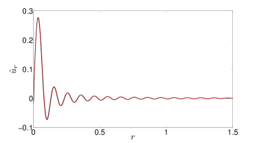
Figure 2: Radial velocity along the $x$-axis for a simulation with forcing amplitude insufficient to cause breaking. The amplitude of this wave is largest in the centre. Also plotted is the corresponding analytic standing wave Eq.67, converted into a radial velocity using Eq.60, showing that our simulations accurately describe the waves for the case in which the waves reflect coherently from the centre.

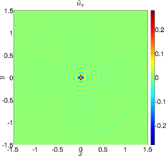
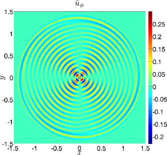
Figure 3: 2D plot of the radial (top) and azimuthal (bottom) velocity in the equatorial plane of the star for small-amplitude waves. This is at a time $t=36t_{c}$, once standing waves have formed, in a simulation with $\mathrm{max}(\tilde{u}_{\phi})<0.3$, in which we have coherent reflection from the centre. In the outer part of the grid, the solution is smoothed to zero to satisfy periodic boundary conditions.

When the simulations are started, transients are excited by the forcing at many different frequencies (and radial wavelengths), centred around $\omega=1$ in frequency space. As more inward propagating waves are excited by the forcing, an ingoing wave train propagates toward the centre. At this stage in the time evolution, the solution is composed of many different frequencies, so our decomposition of the solution into a single IW and OW does not work well. As more transients escape the region and are damped, the primary response of the fluid is in the form of waves with frequency $\omega=1$ and azimuthal wavenumber $m=2$.

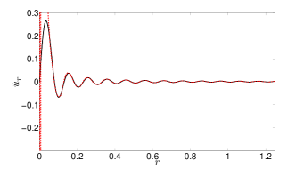
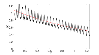
Figure 4: Radial velocity along the line $y$-axis (top) and azimuthal velocity along the line $y=x$ (middle top) in a small-amplitude simulation, after standing waves have been set up at $t=36t_{c}$, with $\mathrm{max}(\tilde{u}_{\phi})\sim 0.3$ (solid lines). Also plotted is the reconstructed solution using $A_{in}$ and $A_{out}$ obtained using the method described in Appendix A (dashed lines). These are well matched everywhere except near the centre showing that our decomposition works well for these cases. In the bottom right we plot $|A_{in}|$ (solid curve) and $|A_{out}|$ (dashed curve) versus radius, together with a linear fit to each curve. The waves damp as they propagate due to viscosity. In the bottom panel we plot the reflection coefficient $\mathcal{R}$ versus radius.

As the waves approach the centre and reflect, an OW is produced. As this process continues, the amplitude of the OW matches that of the IW near the centre. For these low-amplitude cases, the phase change on reflection is negligible. This means that we have coherent reflection from the centre, which allows standing waves to be produced. These waves are stationary in a frame rotating with $\Omega_{p}$, as inferred from linear theory. We confirm that our simulations produce the correct standing wave solution, by plotting an example of a comparison between the simulation and the wave solution in Fig. 2. We plot the velocity components in two dimensions for an example simulation in which standing waves have formed for a small-amplitude case with $\mathrm{max}(\tilde{u}_{\phi})\sim 0.3$ in Fig. 3.

After a few wave crossing times, the reflection coefficient increases to values approaching unity throughout the grid, though its value decreases with radius, shown in Fig. 4 for a low-amplitude case, with $\mathrm{max}(\tilde{u}_{\phi})\sim 0.3$. In this figure we also plot the results of our IW/OW decomposition in a small-amplitude simulation with a resolution $1536\times 1536$. Our reconstructed solutions match the data well except very close to the centre, thus showing that our decomposition works well for these cases.

The decay in $\mathcal{R}$ with radius is a result of the nonzero viscosity, which results in a decay of wave amplitude with time (and therefore distance from where they are excited). The OW has been damped for longer, which results in the amplitude of the OW being smaller than that of the IW. A simple estimate of the amplitude decay due to viscosity with propagation from radius $r$ and then reflected back to $r$ again gives

$$\frac{u_{r}}{u_{r,0}}\propto\exp\left(-2\int_{0}^{r}\frac{\nu k^{2}}{c_{g,r}}dr\right)\approx\exp\left(-\frac{16\pi^{3}\nu}{\omega\lambda_{r}^{3}}r\right),$$ (90)

since $k\sim k_{r}$ except near the centre, and $c_{g,r}\simeq\omega\lambda_{r}/2\pi$ throughout the box. This roughly matches the amplitude decay between $A_{in}$ and $A_{out}$ at $r=1.2$, implying that the decay in amplitude is indeed due to viscous damping of the waves. In addition, the regular oscillations in the amplitudes result from the fact that our exact solution in the inviscid case is not an exact solution in the presence of viscosity. This was verified by running a low-amplitude simulation with $\nu=0$, in which case the oscillations disappear.

We find that the wave reflects coherently from the centre when $\tilde{u}_{\phi}\lesssim 0.5$. Long-term simulations ($t\sim$ several hundred $t_{c}$) do not show the development of any instabilities that act on waves with $\tilde{u}_{\phi}\lesssim 0.5$, though there is a slow growth of $m=0$ components of $\tilde{u}_{\phi}$ in the solution, as can be seen in Fig. 5. In this figure, we plot $P_{m}$ for the first few even wavenumbers in the flow from an example low-amplitude simulation. Negligible growth in odd $m$-values is observed, which is consistent with the symmetry of the basic wave and the quadratic nonlinearities of the Boussinesq-type system. The growth in $m=0$ is a result of viscosity, which acts to damp the waves and transfer angular momentum from $m=2$ to the mean flow. This can distinguished from a process resulting from nonlinear interactions, because it is found to depend on $\nu$. However, most importantly, no instability is observed for waves with $\tilde{u}_{\phi}\lesssim 0.5$.

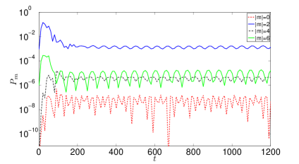
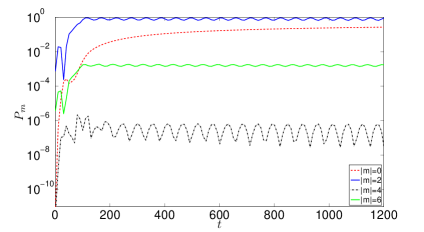
Figure 5: Temporal evolution of the power spectral density $P_{m}$ at $r=0.1$, in the lowest four azimuthal wavenumbers $m$ in the solution for $u_{r}$ (top) and $u_{\phi}$ (bottom), in a low-amplitude simulation with $\tilde{u}_{\phi}\sim 0.3$ near the centre, for grid resolution $512\times 512$. The solution is in the form of $m=2$ waves, and reaches a steady state in the frame rotating with $\Omega_{p}$. Growth of $m=0$ is nonzero as a result of viscous damping of the waves. No wave breaking occurs because $\tilde{u}_{\phi}<0.5$ in the solution. The $m=6$ components are most likely due to errors in the Fourier analysis.

9 High-amplitude forcing: wave breaking and critical layer formation

If we increase the value of $\tilde{f}_{r}$, then the above picture changes considerably when a critical wave amplitude is exceeded. Once $\tilde{u}_{\phi}>\tilde{u}_{\phi,crit}\approx 0.5$, wave breaking occurs near the centre within several wave periods (a few $2\pi/\omega$), and the outcome of the simulations is very different from the small-amplitude case. This occurs when the wave overturns the stratification – see Eqs. 74 and 82. In Fig. 6 we plot the 2D velocity components after wave breaking has occurred in a simulation with $\tilde{f}_{r}=15$.

For highly nonlinear forcing, for example with $\tilde{f}_{r}>20$, the waves break as they reach the centre with sufficient amplitude before there has been any significant reflection. For $\tilde{f}_{r}\sim 10$, the amplitude of the IW alone is insufficient to cause breaking, and we must wait for reflection at the centre to produce an OW of comparable amplitude before $\tilde{u}_{\phi}>\tilde{u}_{\phi,crit}$. Once this critical value of $\tilde{u}_{\phi}$ is exceeded, the waves break. This is an irreversible deformation of the otherwise wavy material contours (McIntyre, 2000).

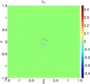
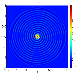
Figure 6: The top panel shows the radial velocity in a high-amplitude simulation with $\tilde{f}_{r}=15$ at $t=7t_{c}$, after wave breaking has occurred, from a simulation with a resolution $1536\times 1536$. The bottom panel shows $\tilde{u}_{\phi}$ at the same time in the simulation.

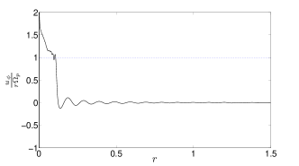
Figure 7: The top panel shows the radial velocity along $y=x$ for the same case as Fig. 6. In the region $r\in[0.3,1.2]$ the solution is well described by linear waves with $|A_{out}|\ll|A_{in}|$, but not near the centre. The bottom panel shows the angular velocity of the fluid normalised to the angular pattern speed of the forcing $\Omega_{p}$ along the $x$-axis, at the same time in the simulation. This shows that the central regions after wave breaking are spun up to slightly exceed $\Omega_{p}$. The critical layer occurs where $u_{\phi}/(r\Omega_{p})=1$.

Once breaking occurs, we observe consequent mean flow acceleration (i.e. growth of $m=0$ components of $u_{\phi}$), as the angular momentum of the waves is deposited locally where the wave breaks. This acts to spin up (if $\Omega_{p}>0$) the central regions, which at this stage contain a sufficiently small fraction of the angular momentum of the star that their spin can be readily affected by these waves. Once this process has begun, the central regions spin up to $\sim\Omega_{p}$, and a critical layer is formed, at which the Doppler-shifted frequency of the waves goes to zero. At this location, the azimuthal phase velocity of the waves would equal that of the local rotation of the fluid, if they were ever to reach it intact. In reality, as subsequent IWs approach the critical layer, nonlinearities dominate, and the waves undergo breaking before they reach it - though see discussion in § 9.2. We plot the angular velocity of the fluid normalised to $\Omega_{p}$ in the bottom panel of Fig. 7.

As IWs approach the critical layer, their radial wavelength decreases, and they slow down, i.e. $\hat{c}_{g,r}\rightarrow 0$ as $\hat{\omega}\rightarrow 0$. This causes a buildup of wave energy just above the critical layer, in which nonlinearities become important. In this thin region, the quadratic nonlinearities produce higher wavenumber disturbances with even $m$ values – see § 9.1. These are produced by the self-nonlinearity of the primary IW ($m=2$) as it approaches the critical layer – these self-nonlinearities vanish in the absence of a mean flow. These daughter waves are damped faster than the primary because they have lower frequencies and therefore shorter radial wavelengths, which is a result of the theorem proved in Hasselmann (1967). Thus the IW is irreversibly deformed, and transfers its angular momentum to either the mean flow or to daughter waves that are then more easily dissipated by viscosity. A large fraction of the angular momentum of these waves must be given to the mean flow when these waves dissipate. This process acts to spin up the fluid just above the critical layer to $\sim\Omega_{p}$. As subsequent IWs are absorbed by the critical layer, the spatial extent of the mean flow expands outwards, i.e. the star is spun up from the inside out. We envisage that this process will continue until the mean flow encompasses the bulk of the radiation zone or the planet plunges into the star – though see § 10. Long-term simulations, lasting for several hundred $t_{c}$, show that this appears to be the case.

This picture is analogous to Goldreich & Nicholson (1989), who propose that early-type stars in close binaries would spin down (if $\Omega>n$, or spin up if $\Omega<n$) from the outside in, once a critical layer has formed near the surface as a result of radiative damping of the waves, where this effect is strong. In our problem, an instability of the primary wave, which occurs once the wave overturns the stratification, causes wave breaking. This results in angular momentum deposition and spin up (for the case in which $\Omega<n$, spin down if $\Omega>n$) of the central regions, which causes the formation of a critical layer near the centre of a solar-type star. The rate of expansion of the spatial extent of this region depends on the forcing amplitude; for larger amplitudes it expands faster. The critical layer moves outwards when the dissipation of subsequent IWs deposits sufficient angular momentum to spin up the fluid to $\sim\Omega_{p}$, and the spatial extent of the mean flow expands. In this picture, there is a front of synchronization which gradually moves outwards (though see § 10).

9.1 Growth of azimuthal wavenumbers in the flow

We now discuss the results of a spectral analysis of the simulation data so that we can study the growth of the mean flow ($m=0$) and daughter waves produced by breaking (other $|m|\neq 2$ wavenumbers). We plot $P_{m}$ for the first few even wavenumbers for a set of examples in Figs. 8 and 9. Negligible growth in odd $m$-values is observed, which is consistent with the symmetry of the basic wave and the quadratic nonlinearities (though it is possible in principle for the wave to be unstable to odd-$m$ perturbations).

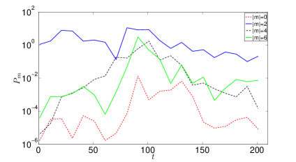
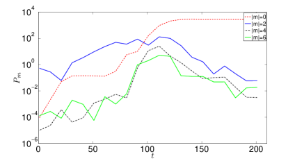
Figure 8: Temporal evolution of the power spectral density $P_{m}$ at $r=0.1$, in the lowest four azimuthal wavenumbers $m$ in the solution for $u_{r}$ (top) and $u_{\phi}$ (bottom), in a simulation with $\tilde{f}_{r}=15$ for resolution $1536\times 1536$. The solution is primarily in the form of $m=2$ waves, until growth of even-$m$ disturbances occurs as the wave breaks. Note that $m=0$ grows strongest for $u_{\phi}$, i.e. angular momentum is transferred from the primary waves to the mean flow. Once $r=0.1$ is located inside the rotating region, $u_{r}$ is primarily composed of $|m|=2$.

At the beginning of the simulations $m=2$ dominates until the primary wave breaks and transfers angular momentum to the mean flow. When subsequent waves approach the critical layer the primary IW transfers angular momentum to higher $m$-value disturbances – this can be seen from Fig. 8 prior to $t\sim 100$, after which the ring $r=0.1$ is enveloped by the mean flow. After this, $m=0$ dominates $u_{\phi}$. On the other hand, $u_{r}$ is then primarily in the form of $|m|=2$ disturbances, which from examination of simulation output, counter-rotate with the forcing, and have angular pattern speed $-\Omega_{p}$. The excitation of these waves could explain the counter-intuitive effect of the most central regions spinning slightly faster than $\Omega_{p}$, since they carry negative angular momentum. These waves appear to reflect from both the $m=2$ critical layer (though note that these waves do not see this as a critical layer) and the centre. As these waves approach the $m=2$ critical layer, since they are counter-propagating waves, their frequency is Doppler-shifted upwards towards $N$, and they undergo total internal reflection. These waves appear to reflect back and forth from the critical layer and the centre.

We also note the appearance of oscillations in the energy in $m=6$ in the solution. This is most likely due to errors in the Fourier analysis, because we are not sampling the solution with evenly spaced points. The amplitude of these oscillations is much smaller than that of the $m=2$ or $m=0$ waves, so should not affect any conclusions drawn from these results.

We experimented with the forcing amplitude to study cases in which wave amplitudes were just sufficient to cause breaking after running the simulation for $\sim 25t_{c}$. The results of our spectral analysis of the results of such a simulation are plotted in Fig. 9. We clearly see evidence for viscous damping in producing growth of energy in $m=0$. This can be distinguished from the sudden growth which results after the onset of the instability that leads to wave breaking. The growth of an instability on the primary wave occurs once the wave overturns the stratification, when $\tilde{u}_{\phi}>\tilde{u}_{\phi,crit}$ near the centre, at $t=2200$. After onset, the wave breaks and a critical layer is formed, leading to the general picture described above. For this simulation, viscous damping of the wave is responsible for spinning up the flow, and the formation of a critical layer.

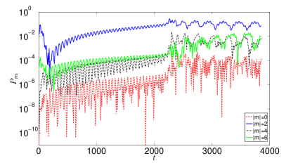
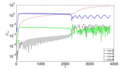
Figure 9: Temporal evolution of the power spectral density $P_{m}$ at $r=0.1$, in the lowest four azimuthal wavenumbers $m$ in the solution for $u_{r}$ (top) and $u_{\phi}$ (bottom), in a simulation with $\tilde{f}_{r}=2.5$ for resolution $512\times 512$. Until $t=2200$, viscous damping acts on the waves, transferring angular momentum to the mean flow. Once $u_{\phi}>u_{\phi,crit}$ in the solution, wave breaking occurs. This occurs at $t\sim 2200$, resulting in a jump in the growth of $m=0$, and a drop of energy in $|m|=2$.

9.2 Discussion of wave reflection from the critical layer and implications

Once the critical layer has formed, we find that a large fraction of the IW angular momentum is absorbed near the centre. First, we confirmed this naively by watching animations of the time dependence of the velocity components. For both components, the wave pattern moves outwards, which corresponds to inward propagating IGWs (see § 5), so at least a significant fraction of the solution is in the form of IWs. This is quantified by performing our IW/OW decomposition. The results of this for a typical simulation are plotted in Fig. 10, where $\tilde{f_{r}}=15$. The time has been chosen after the critical layer has formed, and the mean flow has been accelerated near the centre. The IW/OW wave decomposition does not work well near the centre, as we might expect, since here the disturbance is primarily the mean flow ($m=0$), though there are also other components. Several wavelengths from the critical layer, in the region $0.5<r<1.2$, the reconstructed wave solution matches the simulation output quite well. The matching is much noisier than in Fig. 4, since the solution contains contributions from $m\neq 2$ wavenumbera and $\omega\neq 1$ frequencies in addition to $m=2$, $\omega=1$ waves.

Fig. 10 shows that the amplitude of the IW decays as it propagates towards the centre. There is significant absorption of wave angular momentum near the critical layer, as the IW propagates through the mean shear. This results in $|A_{out}|\ll|A_{in}|$, though the reflection is nonzero so $|A_{out}|\neq 0$. This leads to $\mathcal{R}\ll 1$ in the region where the decomposition works well, which implies that most of the angular momentum in the IWs is absorbed near the centre – also note that the energy flux ratio $\propto\mathcal{R}^{2}\ll 1$. In addition, the phase of the OW is perturbed with respect to the IW, which inhibits the formation of standing waves. $\mathcal{R}$ oscillates with radius, mainly because the solution is composed of some $\omega\neq 1$ and $m\neq 2$ components, which are not filtered by our IW/OW decomposition.

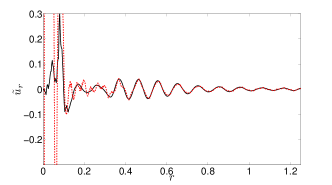
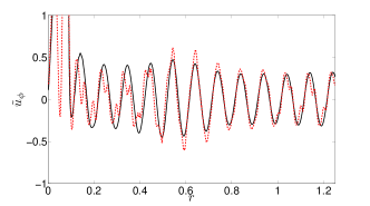
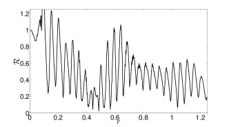
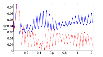
Figure 10: Radial velocity along the line $y=x$ (top) and azimuthal velocity along the $x$-axis (middle top) in a large-amplitude simulation with wave breaking, at $t=7t_{c}$, with $\tilde{f}_{r}=15$. These are plotted (solid lines) together with the reconstructed solution using $A_{in}$ and $A_{out}$ obtained from the method described in Appendix A (dashed lines) – these are well matched for $r\in[0.5,1.2]$. Bottom right panel shows $A_{in}$ (top line) and $A_{out}$ (bottom line) vs radius. There is significant absorption of IWs near the critical layer at $r\sim 0.1$, resulting in $|A_{out}|\ll|A_{in}|$. The bottom panel shows the reflection coefficient $\mathcal{R}$ versus radius. $\mathcal{R}\ll 1$ in the region where the decomposition works well.

When a single propagating wave approaches a critical layer, the outcome has previously been found to depend on the ratio of the strength of nonlinear wave-wave couplings to linear viscous and radiative damping. Nonlinear wave-wave couplings occur over a timescale (Booker & Bretherton, 1967)

$$t_{NL}=O\left(k_{h}^{-\frac{2}{3}}|\partial_{r}U_{h}|^{-\frac{1}{3}}U_{r}^{-\frac{2}{3}}\right),$$ (91)

and linear viscous and radiative damping occur over a timescale

$$t_{L}=O\left(k_{h}^{-\frac{2}{3}}\nu^{-\frac{1}{3}}|\partial_{r}U_{h}|^{-\frac{2}{3}}\right).$$ (92)

The ratio of these terms define the parameter (Maslowe 1986; Koop 1981)

$$\lambda\equiv\frac{t_{NL}}{t_{L}}\sim\left(\frac{\nu|\partial_{r}U_{h}|}{U^{2}_{r}}\right)^{1/3}.$$ (93)

where $k_{h}$ is the horizontal wavenumber, $\partial_{r}U_{h}$ is the typical shear in the mean flow, $U_{r}$ is a typical radial velocity in the wave, and $\nu$ is a diffusivity – which for the centre of a star is likely to be primarily radiative diffusion rather than viscosity, so $\nu$ will be primarily the thermal conductivity $\kappa$.

Nonlinearity acts to promote energy transfer away from the critical layer through the generation of daughter waves, and linear damping acts to suppress this resonant wave production. If $\lambda\gg 1$, then the time required for nonlinear effects to become important is long compared with that for linear damping to become important. In this limit, there is negligible wave reflection, and nearly all incoming wave energy is absorbed by the critical layer, as predicted by Hazel (1967). In the opposite limit, when $\lambda\ll 1$, nonlinear effects become manifest prior to the time when they become suppressed by linear damping. In this case, the flow can be extremely complicated, and nonlinearity in the critical layer region can lead to wave reflection, with ampltiudes $O\left(\exp\left(-\pi(Ri-1/4)^{1/2}\right)\right)$ or less (Breeding, 1971). In this limit, nonlinear wave-wave couplings lead to the generation of many smaller-scale daughter waves, some of which propagate away from the critical layer, carrying a fraction of the wave energy (Fritts, 1979). Experiments of internal waves approaching a critical layer have been performed by Koop (1981) and Koop & McGee (1986), in which $\lambda=O(1)$. For this value, the effects of both nonlinearity and linear damping become manifest at approximately the same time. Their laboratory experiments show that wave reflection, in the form of daughter waves produced by nonlinear couplings that propagate away from the critical layer, is suppressed by viscosity for this value of $\lambda$.

Relating these results to our simulations, we find typical values of the parameter $\lambda\sim 10^{-1}$ near the critical layer, due to the explicit viscosity ($\nu=2\times 10^{-6}$) added in the code, since $|\partial_{r}U_{h}|\sim O(10^{1})$ and $U_{r}=\tilde{u}_{r}\sim 0.1$. In this limit nonlinearities are likely to become important before viscous diffusion. Since this is the limit in which we would be expected to find wave reflection, if any occurs at all, and we find little reflection of waves from the critical layer, it is likely that most of the IWs are absorbed near to the centre, and not reflected. In any case, the reflected waves will not have the same frequency and horizontal wavenumber as the primary wave. Instead, reflected waves will be in the form of disturbances with smaller frequencies, and therefore shorter radial wavelengths, as well as higher $m$-values, as a result of wave-wave coupling (Hasselmann, 1967). Such disturbances will be more easily dissipated by radiative diffusion, since the rate of energy dissipation $\sim m^{3}/\omega^{4}$.

We conclude that if wave breaking and critical layer formation occurs, it is probably reasonable to assume that the IWs are entirely absorbed in the radiation zone, primarily near to the critical layer. This is inferred from our simulations, as can be seen in the example in Fig. 10, in which $|A_{out}|\ll|A_{in}|$. The result of this is that if wave breaking and critical layer formation occurs, it is not possible for global standing modes to develop in the radiation zone. It would then be appropriate to calculate the tidal dissipation rate using the method of GD98.

10 Discussion

10.1 Orbital evolution of the planetary companion

The main motivation for our work is to study the tidal $Q^{\prime}$ expected for solar-type stars, and in particular to connect this with the survival of close-in extrasolar planets. If the amplitude of the tide is sufficient to excite IGWs that exceed the critical amplitude for wave breaking at the centre, then our results find it highly likely that the wave reflection will be imperfect, and a large fraction of the incoming wave energy will be absorbed. It is then reasonable to estimate the amount of tidal dissipation by assuming that the incoming waves are completely absorbed. This was first done by GD98 for a nonrotating solar model, and we here reproduce the relevant quantities to calculate $Q^{\prime}$ using their approach. The energy flux $F$ in ingoing IGWs excited at the convective/radiative interface (at radius $r=r_{int}$) is (see GD98 Eq. 13)

$$F = \beta\mathcal{G}\omega^{\frac{11}{3}},$$ (94)

where $\omega=2n$ is the frequency of IGWs excited by a planet in a circular, nonsynchronous orbit,

$$\beta = \frac{3^{\frac{2}{3}}}{8\pi}\left[\Gamma\left(\frac{1}{3}\right)\right]^{2}\left[l(l+1)\right]^{-\frac{4}{3}}$$ (95)

is a constant (for quadrupolar tides $l=2$), and

$$\mathcal{G} = \left[\rho r^{5}\left|\frac{dN^{2}}{d\ln r}\right|^{-\frac{1}{3}}\left|\frac{\partial\xi_{r}}{\partial r}\right|^{2}\right]_{r=r_{int}}=\tilde{\mathcal{G}}\frac{2\pi\Psi^{2}}{\omega_{dyn}{{}^{4}}},$$ (96)

where $\tilde{\mathcal{G}}$ depends on the stellar properties at the interface between radiative and convective regions, and

$$\frac{dN^{2}}{d\ln r}(r_{int}) \approx -100\omega^{2}_{dyn},$$ (97)

$$\frac{\partial\xi_{r}}{\partial r}(r_{int}) \approx \sigma_{c}\frac{\Psi}{\omega^{2}_{dyn}},$$ (98)

and $\sigma_{c}$ is a constant whose value depends primarily on the thickness of the convection zone, and is equal to -1.2 for the current Sun. The values of these quantities depend on the stellar model. The amplitude of the largest tide for a circular orbit is (e.g. OL04)

$$\Psi=\sqrt{\frac{3}{5}}\frac{m_{p}}{(m_{\star}+m_{p})}n^{2},$$ (99)

if the tidal potential has the form $\mathrm{Re}[\Psi r^{2}\tilde{P}^{m}_{2}(\cos\theta)e^{i(m\phi-\omega t)}]$, where $\tilde{P}^{m}_{2}$ corresponds to the Legendre polynomial of degree 2 normalised over $\theta$ (related to the spherical harmonic $Y_{2,m}=(1/\sqrt{2\pi})\tilde{P}^{m}_{2}e^{im\phi}$). Converting the energy flux $F$ to an angular momentum flux, and assuming all wave angular momentum is deposited in the star, we calculate a torque $T$, using the torque formula given in Peale (1999), giving

$$T=\frac{m}{\omega}F=\frac{9}{4}\frac{1}{Q^{\prime}_{\star}}\left(\frac{m_{p}}{m_{\star}+m_{p}}\right)^{2}\frac{m_{\star}R_{\star}^{2}}{\omega_{dyn}^{2}}n^{4},$$ (100)

where $m=2$. Then

$$Q^{\prime}_{\star} = \frac{15}{32}\frac{3^{\frac{2}{3}}}{\pi^{\frac{8}{3}}}\frac{1}{\left[\Gamma(\frac{1}{3})\right]^{2}}\frac{1}{\tilde{\mathcal{G}}}m_{\star}R_{\star}^{2}\omega_{dyn}^{2}P^{\frac{8}{3}}$$ (101)

$$\approx 1.5\times 10^{5}\left[\frac{P}{1\;\mathrm{day}}\right]^{\frac{8}{3}},$$ (102)

where $P$ is the orbital period, which is twice the tidal period for the diurnal component of the tide. Note that the exact value depends on the stellar model adopted – in particular the value of $\tilde{\mathcal{G}}$, which is determined from the stellar properties at the interface between radiative and convective regions, and the thickness of the convection zone. The given value applies to a stellar model of the current Sun (see below for a discussion of the variation in this parameter for other stars). The largest uncertainty is likely to be in $\left|\frac{dN^{2}}{d\ln r}\right|^{-\frac{1}{3}}$, since this may depend on the modelling of convective overshoot. However, uncertainties in $\tilde{\mathcal{G}}$ for the current Sun are much less than an order of magnitude, so this is a good estimate of $Q^{\prime}_{\star}$ that results from the mechanism described in this paper, for our closest star.

We now estimate the orbital and stellar properties required to excite waves that are sufficiently nonlinear near the centre for breaking to occur, using the Appendix of OL07 and the above energy flux. The nonlinearity parameter in OL07 is defined so that for $A>1$, the wave overturns the stratification during part of its cycle. Equating the energy flux in ingoing waves near the centre to Eq. 94 gives

$$A = \frac{3}{20}\frac{3^{\frac{5}{12}}\Gamma(\frac{1}{3})}{2^{\frac{1}{4}}\pi^{\frac{2}{3}}}\frac{\tilde{G}^{\frac{1}{2}}}{\omega_{dyn}^{2}}\left(\frac{C^{5}}{\rho_{c}}\right)^{\frac{1}{2}}\left(\frac{m_{p}}{m_{\star}+m_{p}}\right)P^{\frac{1}{6}}$$ (103)

$$\approx 0.3\left(\frac{\tilde{\mathcal{G}}}{\tilde{\mathcal{G}}_{\odot}}\right)^{\frac{1}{2}}\left(\frac{C}{C_{\odot}}\right)^{\frac{5}{2}}\left(\frac{m_{p}}{M_{J}}\right)\left(\frac{M_{\odot}}{m_{\star}}\right)\left(\frac{P}{1\;\mathrm{day}}\right)^{\frac{1}{6}},$$ (104)

where $\tilde{\mathcal{G}}_{\odot}\approx 2\times 10^{47}\mathrm{kg}\,\mathrm{m}^{2}\mathrm{s}^{2/3}$ and $C_{\odot}\approx 8\times 10^{-11}\mathrm{m}^{-1}\mathrm{s}^{-1}$. If we assume that the primary instability acting on 3D waves occurs for the minimum amplitude at which the 3D wave solution overturns the stratification ($A>1$), which we have found is indeed the case in 2D, then we have the following criterion for wave breaking:

$$\left(\frac{\tilde{\mathcal{G}}}{\tilde{\mathcal{G}}_{\odot}}\right)^{\frac{1}{2}}\left(\frac{C}{C_{\odot}}\right)^{\frac{5}{2}}\left(\frac{m_{p}}{M_{J}}\right)\left(\frac{M_{\odot}}{m_{\star}}\right)\left(\frac{P}{1\;\mathrm{day}}\right)^{\frac{1}{6}}\gtrsim 3.3.$$ (105)

A Jupiter-mass planet in a one-day orbit around the current Sun would not raise tides of sufficient amplitude near the centre for breaking to occur, and would likely survive, because it does not satisfy this criterion. Note, however, that Jupiter, with its period of $P=4332$d, does satisfy this criterion. The waves excited by Jupiter in the Sun would be of very low amplitude, but they are also of very low frequency. This means that their wavelength is extremely short, so the energy of these waves would be concentrated into an extremely small volume near the centre of the star, if they were to reach it. However, radiative diffusion is certain to damp these waves before they reach the centre, since they are of such short wavelength. This process would, in any case, contribute negligibly to the orbital evolution of Jupiter.

We performed a study of the variation in the parameters $\tilde{\mathcal{G}}$ and $C$ using an extensive set of stellar models, with masses $0.5\leq m_{\star}/M_{\odot}\leq 1.1$, and ages that represent the range of main-sequence ages expected for these stars. These were provided by Jørgen Christensen-Dalsgaard, and were computed using ASTEC (Christensen-Dalsgaard, 2008). This involved integrating GD98 Eq.(3) throughout the convection zone in each of these models, where $N\sim 0$, using a linear shooting method, to determine $\sigma_{c}$. The results of this study are that $\tilde{\mathcal{G}}\sim\tilde{\mathcal{G}}_{\odot}$ to within a factor of 5 for all solar-type stars, throughout the main-sequence age of each star. This is true even taking into account the evolution of the position of the interface between convection and radiation zones, and the resulting change in the density of the star at the interface. The main uncertainty in each model is probably $\left|\frac{dN^{2}}{d\ln r}\right|$ at the interface, since the slope of $N^{2}$ there is uncertain. However, this is only raised to the -1/3 power, so this effect probably does not contribute more than a factor of 2 uncertainty in $\tilde{\mathcal{G}}$. Taken together with changes in stellar mass and radius, we find that our estimate of $Q^{\prime}_{\star}$ in Eq. 102 is quite robust, if critical layer formation occurs at the centre. This is approximately true for all stars within the mass range $0.5\leq m_{\star}/M_{\odot}\leq 1.1$, throughout their main-sequence lifetime.

The variation in $A$ is primarily dependent on $C$, since $A\propto\tilde{\mathcal{G}}^{\frac{1}{2}}C^{\frac{5}{2}}$. The strong dependence on $C$ means that as a star evolves the tide could become nonlinear at a critical age, since $C$ increases with evolution on the main-sequence (see Fig. 1 for the evolution of $C$ with the age of the Sun). For a given age, this parameter is found to be larger in more massive stars, due to their greater central condensation. In addition, stars with lower metallicity also have a greater central condensation for a given age, and so have larger $C$ values over stars with higher metallicity. Over the range of stars considered in this study, $C$ is found to take values between $0.1-10C_{\odot}$. This leads to a large variation in $A$ values, for fixed orbital parameters. As a result, this parameter is critical in determining whether wave breaking occurs at the centre. We have stated that a short-period Jupiter-mass planet does not satisfy Eq. 105 around the current Sun. However, such a planet around a similar age $1.0M_{\odot}$ star with a metallicity $Z=0.01$ will cause wave breaking at the centre, since $C$ is larger by a factor of 3. Thus, there is a strong dependence of the breaking criterion on the stellar model, primarily through the parameter $C$.

Tidal dissipation of the quadrupolar tide raised in the star leads to evolution of the semi-major axis at the rate

$$\frac{\dot{a}}{a}=-\frac{9}{2}\left(\frac{R_{\star}}{a}\right)^{5}n\left[\frac{\mathrm{sgn}(2n-2\Omega)}{Q^{\prime}_{\star}}\right].$$ (106)

The inspiral time for a planet into the current Sun is then

$$\tau_{a}=-\frac{2}{21}\frac{a}{\dot{a}}\approx 2.3\;\mathrm{Myr}\left(\frac{M_{J}}{m_{p}}\right)\left(\frac{M_{\odot}}{m_{\star}}\right)^{\frac{5}{6}}\left(\frac{R_{\odot}}{R_{\star}}\right)^{5}\left(\frac{P}{1\;\mathrm{day}}\right)^{7}$$ (107)

since $\dot{a}/a\propto a^{-21/2}$. Note that the strong frequency dependence of $Q^{\prime}_{\star}$ means that this mechanism could be very important for short-period systems. This predicts that a planet spiralling into its star will undergo rapid acceleration as it migrates inwards. This is as a consequence not only of the reduction in semi-major axis, but also the decrease in $Q^{\prime}_{\star}$ as the tidal frequency increases with the inspiral. It must be noted that simple timescale estimates do not accurately reflect the evolution if the orbit is eccentric, inclined, or if the stellar spin is not much slower than the orbit (Barker & Ogilvie, 2009), but this estimate shows that this mechanism can be very efficient in contributing to the tidal evolution of hot Jupiters on the tightest orbits. Indeed, $\tau_{a}<5$ Gyr for a Jupiter-mass planet in an orbit of less than about three days around the current Sun, if it were to cause wave breaking near the centre.

We can crudely estimate the maximum orbital period of a planet that can be pulled into the star by this process by equating the moments of inertia of the radiation zone (which extends to radius $R_{RZ}$), to that of the orbit $\mu a^{2}=r_{g}^{2}m_{\star}$, giving

$$P\simeq 1.8\;\;\mathrm{days}\left(\frac{m_{\star}}{M_{\odot}}\right)^{\frac{1}{2}}\left(\frac{R_{RZ}}{0.7R_{\odot}}\right)\left(\frac{M_{J}}{\mu}\right)^{\frac{1}{2}},$$ (108)

where $\mu=\frac{m_{p}m_{\star}}{m_{p}+m_{\star}}$ is the reduced mass and $r^{2}_{g}=0.076$ is the dimensionless radius of gyration for a polytrope of index 3. For a planet with such an orbital period, the whole of the radiation zone must be spun up to cause the planet to completely spiral into the star. Once the entire radiation zone has spun up to the orbital frequency, this process becomes ineffective and the corresponding tidal torque will vanish. However, the tidal torque is nonzero due to dissipation of the equilibrium tide by turbulent convection, and so even if this process stops, it does not guarantee the survival of the planet. In addition, magnetohydrodynamic coupling between the convection and radiation zones could act to partially counteract the spin-up of the interior, if the convection zone is spinning slower than the orbit. Magnetic braking of the star through the interaction of its magnetic field with a stellar wind acts to spin down the convection zone, which would also gradually spin down the radiation zone through these couplings. If the coupling between the convection and radiation zones of the star is efficient, then our mechanism would again become effective. In the case that the coupling timescale balances the timescale for spin up of the radiation zone due to IGW absorption at a critical layer, then the planet would migrate into the star on the magnetic braking timescale. A detailed study of these effects is not currently possible, since there are many uncertainties, but this is worthy of future consideration.

A Jupiter-mass planet on a $\sim 1$ day orbit will spin up a substantial fraction of the radiation zone on infall. If the ratio of the orbital moment of inertia to the spin moment of inertia of the radiation zone $\gtrsim 1$, then the above process alone will be unable to cause the planet to spiral into the star.

10.2 Critical layer formation induced by radiative diffusion

Near the centre of a star, radiative diffusion is the dominant linear dissipation mechanism. If the waves are sufficiently attenuated by radiative diffusion on their reflection from the centre, then over a sufficiently long time, they may be able to spin up the innermost regions of the star to the angular pattern speed of the tide $\Omega_{p}$, hence producing a critical layer. We have already observed this process occuring in our simulations in Fig. 9, albeit with viscosity and not radiative diffusion acting on the waves. Here we provide an order-of-magnitude estimate of the timescale for this process.

If we assume that the wave is attenuated as it propagates from a radius $R$, to the centre, and back to $R$ again, by a factor $e^{-\alpha}$, i.e., that the energy flux is $Fe^{-\alpha}$, then the torque on this region of the star is given by the angular momentum transferred to the mean flow, and is

$$T=\frac{m}{\omega}F(1-e^{-\alpha}).$$ (109)

Here we assume that $F$ is that given in Eq. 94, which is probably reasonable when the response is non-resonant. The wave attenuation $\alpha$ is given by

$$\alpha\approx 2\int_{0}^{R}\frac{\eta_{rad}k^{2}}{c_{g,r}}dr,$$ (110)

where $\eta_{rad}$ is the thermal conductivity, $k$ is the wavenumber. We have $k\sim k_{r}$ except within the last wavelength from the centre, and the radial group velocity $c_{g,r}\approx\frac{\omega}{k_{r}}$. The thermal conductivity can be calculated from the properties of the appropriate stellar model from

$$\eta_{rad}=\frac{16\sigma T^{3}}{3\kappa\rho^{2}c_{p}},$$ (111)

where $\sigma$ is the Stefan-Boltzmann constant, $\kappa$ is the opacity, and $c_{p}$ is the specific heat at constant pressure. We can take $\eta_{rad}$ to be constant over the inner $\sim 3\%$ of a star, to a first approximation, with a value $\approx 16.7\mathrm{m}^{2}\mathrm{s}^{-1}$ in the case of the Sun. In addition, $k_{r}$ is roughly constant with radius within this region, though diverges as $r\rightarrow 0$. We can reasonably estimate

$$\alpha\approx 2\times 6^{\frac{3}{2}}\eta_{rad}\frac{C^{3}}{\omega^{4}}R\approx 4\times 10^{-4}\left(\frac{R}{R_{\odot}}\right)\left(\frac{P}{1\mathrm{d}}\right)^{4}$$ (112)

where $R$ is the size of the region spun up by this process. This is because $k_{r}\sim\frac{\sqrt{l(l+1)}N}{r\omega}$, if $\omega\ll N$, and $N=Cr$. We also note that the tidal frequency $\omega=2\left(\frac{2\pi}{P}\right)$. This means that the attenuation by radiative diffusion within the innermost few percent of the star, is small for waves excited by planets on one-day orbits. However, the wavelength of the waves becomes shorter for longer period orbits, so their attenuation by radiative diffusion is more efficient. Note that $\alpha\gtrsim 1$ only when $P\gtrsim 8$ days, even when radiative diffusion over the entire radiation zone is considered (in fact GD98, who made a more accurate calculation by including the radial dependence of the wavenumber and diffusivity, found that $\alpha\gtrsim 1$ for $P\gtrsim 11.6$ days). This means that the waves excited by planets on short-period orbits with $P\lesssim 3$ days, whose survival could be threatened by the process of wave breaking, will not be significantly attenuated in traversing the radiation zone, according to linear theory. It is therefore appropriate to ask whether they will break on reaching the stellar centre.

To a first approximation, the central $\sim 3\%$ of a star can be modelled as a uniform density sphere, with the central density $\rho_{c}$. Its moment of inertia is $I=\frac{4}{5}\pi R^{5}\rho_{c}$. Using Eq. 109, we have the following differential equation describing the spin evolution of the central regions:

$$I\frac{d\Omega}{dt}=\frac{m}{\omega}F(1-e^{-\alpha}).$$ (113)

Assuming that the system evolves slowly, which is probably true until breaking occurs, we can take $F$, $\omega$, and $\alpha$, to be constant in time as the central regions are spun up. This allows a straightforward solution, giving the resulting timescale to spin up the region of the central wavelength to $\Omega_{p}$, in the case of Jupiter orbiting the Sun with a one-day period (in which $R\sim 0.01R_{\odot}$), of

$$t_{SU}=\frac{4}{5}\frac{\pi R^{5}\rho_{c}\Omega_{p}^{2}}{F(1-e^{-\alpha})}\approx 3\;\mathrm{Myr}.$$ (114)

Note that this timescale strongly depends on the size of the region that is spun up. When $\alpha\ll 1$, which is valid for $P\lesssim 10$ days, $t_{SU}\propto P^{5/3}$.

In this estimate we have used Model S of the current Sun, so this value only applies to our star. However, we have repeated this calculation using the same set of stellar models discussed in the previous section, with masses in the range $0.5\leq m_{\star}/M_{\odot}\leq 1.1$, and find that $t_{SU}\lesssim 1$ Gyr for each of these models, for Jupiter orbiting the star with a one-day period.

This striking estimate indicates that all gas giants on short-period orbits around G or K stars could eventually cause the formation of a critical layer near the centre of the star, given sufficient time $\lesssim O(1)$ Gyr. Once this has formed, we have found in our simulations in §7, that it is reasonable to assume that the ingoing wave angular momentum flux is entirely absorbed near the centre. Hence, our estimate of $Q_{\star}^{\prime}$ in the previous section could apply to all slowly rotating G and K stars. The effects of rotation will complicate matters if the tidal frequency is less than twice the spin frequency, as studied in OL07.

Unlike the mechanism of nonlinear wave breaking, which is the main subject of this paper, the formation of a critical layer by radiative diffusion requires the progressive spin-up of the region of the central wavelength by a very gradual deposition of angular momentum. This process could be interrupted by other mechanisms of angular momentum transport that resist the development of differential rotation, such as hydrodynamic instabilities or magnetic stresses. A consideration of such effects will be required in order to determine whether this process operates in reality.

10.3 Long-term evolution of the radiation zone

As the planet migrates inwards due to the IGWs it excites being absorbed at a critical layer, $\omega$ increases, since $\dot{n}>0$. If we assume that the tidal frequency increases from $\omega_{1}$ at a time $t_{1}$ to $\omega_{2}>\omega_{1}$ at a slightly later time $t_{2}$, then since $\omega_{2}>\omega_{1}$, the waves excited at $t_{2}$ no longer see the critical layer for $\omega_{1}$ waves. If the change in frequency is sufficiently small, we would still expect significant attenuation by the shear as the waves approach the critical layer for $\omega_{1}$ waves. This would transfer angular momentum from the waves to the mean flow, and may spin up the region near the original critical layer to the pattern speed for $\omega_{2}$ waves, hence producing a critical layer for these waves. If this process occurs, then a weak radial differential rotation profile could be set up in the radiation zone, with $\frac{d\Omega(r)}{dr}>0$. Similarly, if the planet migrates outwards, then a profile with $\frac{d\Omega(r)}{dr}<0$ could be set up. If the flow does not have time to adjust to the change in frequency of the forcing, and cannot spin up sufficiently to produce a critical layer for $\omega_{2}$ waves, then the dissipation rate may be reduced. However, it seems plausible that the change in the orbit will be gradual enough so that IGWs reaching the centre will be significantly attenuated. This is because their radial wavelengths get Doppler-shifted downwards by the shear, making them more susceptible to radiative damping.

We have so far restricted our investigation to $m=2$ waves. If the orbit of the planet is eccentric or inclined with respect to the stellar equator, then IGWs with other $m$-values could be excited. If these break, then they could each have their own critical layer. It would be interesting to study the effects of tidal forcing with several different frequencies and $m$-values to see how this would affect the reflection of the different waves. In addition, Rogers & Glatzmaier (2006) found that IGWs excited by turbulent convection at the top of the radiation zone, which had $1<m<15$ and typical frequencies $\omega\sim 20\mu$Hz, could reach the centre with sufficient amplitude to undergo breaking and spin up the central regions. If this commonly occurs in solar-type stars, then we might expect the core to be differentially rotating, even in the absence of tidal forcing. For most $m$-values the resulting spin frequency of the central regions is probably slower than that of the relevant pattern speed for tides raised by a close-in planet, so we expect that this would minimally attenuate any tidally excited low-$m$ waves. Nevertheless, the interactions of multiple waves near the centre warrants further study.

11 Conclusions

We have presented a study of the fate of internal gravity waves approaching the centre of a solar-type star, primarily using two-dimensional numerical simulations. A train of internal gravity waves excited at the interface between the convection and radiation zones propagates towards the centre. These waves break if they reach the centre with steepness sufficient to overturn the stratification, which in 2D corresponds to $\tilde{u}_{\phi}>\tilde{u}_{\phi,crit}\sim 0.5$. Once this occurs, nonlinear effects cause the subsequent formation of a critical layer, as the waves transfer their angular momentum to the mean flow, bringing the central regions of the star into corotation with the tidal forcing. This acts as an absorbing barrier for subsequent ingoing waves, which continue to be absorbed near the critical layer, resulting in an expansion of the spatial extent of the mean flow. The general picture of this process is that the star spins up (or down) from the inside out, until either the planet has plunged into the star, or the radiation zone of the star has spun up (or down) to match that of the evolving orbit.

In 2D, wave breaking occurs near the centre if $\tilde{u}_{\phi}\gtrsim 0.5$. The amplitude of gravity waves excited by tidal forcing have this value near the centre of the current Sun if

$$\left(\frac{m_{p}}{M_{J}}\right)\left(\frac{P}{1\;\mathrm{day}}\right)^{\frac{1}{6}}\gtrsim 3.3.$$ (115)

However, this value depends strongly on the stellar model, in particular the value of $\frac{dN}{dr}$ at the centre, which varies between different stars, and with main-sequence age. It is likely that a short-period Jupiter-mass planet will not excite waves with sufficient amplitude to cause breaking near the centre of the current Sun, since it does not satisfy this criterion. There is also a dependence on the stellar properties at the interface between convection and radiation zones (see Eq. 105). However, the uncertainties in these parameters are expected to be markedly less than an order of magnitude, given a stellar mass and approximate age (and metallicity).

By decomposing the numerical solutions into an ingoing and outgoing wave, we find that if wave breaking occurs most of the angular momentum of the ingoing wave is absorbed near the centre, and is not reflected. This has very important implications for tidal dissipation in solar-type stars. We find that the assumption of GD98 and OL07, that tidally excited internal gravity waves approaching the centre a star are not coherently reflected, and do not produce standing modes, is appropriate. Neglecting the effects of rotation, we use the calculations of GD98 (with the minor corrections of OL07) to estimate the modified tidal quality factor that results from dissipation of these waves near the centre. Its value is

$$Q^{\prime}_{\star}\approx 1.5\times 10^{5}\left[\frac{P}{1\;\mathrm{day}}\right]^{\frac{8}{3}},$$ (116)

for the current Sun. This mechanism produces efficient tidal dissipation over a continuous range of tidal frequencies, once wave breaking occurs. If wave breaking does not occur, the wave is perfectly reflected from the centre, and global standing modes can be set up in the radiation zone. In this case, efficient dissipation only occurs when the tidal frequency becomes resonant with a global standing mode, but this contributes negligibly to the dissipation, since the system moves rapidly through these resonances (Terquem et al., 1998).

From studying an extensive set of stellar models, this estimate of $Q^{\prime}_{\star}$ is found to vary by no more than a factor of 5 between all main-sequence stars, with masses in the range $0.5-1.1M_{\odot}$, at any stage in their main-sequence lifetime. This means that our estimate is quite robust, and is likely to apply to all G and K stars within the mass range $0.5-1.1M_{\odot}$, at any stage in their main-sequence lifetime (as long as they do not possess a convective core).

The strong frequency dependence of $Q^{\prime}_{\star}$ implies a rapid ($\sim 1$ Myr) and accelerating inward migration of planets on the tightest orbits around solar-type stars, if these planets excite waves with sufficient amplitudes to cause breaking. These planets can spiral completely into their stars if their orbital moment of inertia is smaller than the spin moment of inertia of the radiation zone. If the planet has a larger moment of inertia than that of the radiation zone, then the planet will spin up the entire radiation zone, and this process will become ineffective in the absence of any competing effects. Consequently, we predict that fewer hot Jupiters which satisfy the breaking criterion, with orbital periods of less than 2-3 days, will be found around solar-type stars. Planets with masses much larger than Jupiter could transfer sufficient angular momentum to the radiation zone before they are engulfed by the star. Further evolution would then depend on the strength of the coupling between the radiation and convection zones, and on magnetic braking of the star through the interaction of its magnetic field with a stellar wind. The outcome that results from the interaction of these effects is uncertain.

Our work is an extension of nonlinear mechanism for tidal dissipation proposed by GD98, and contributes several new results. While their model was applied to the circularisation of close binary stars, we (following OL07) focus on the inward tidal migration of short-period extrasolar planets. We have performed numerical simulations, which clearly determine the criterion for wave breaking in two dimensions. Furthermore, we have found that the resulting spin-up of the central regions of the star leads to an ongoing tidal torque as incoming waves are absorbed in a critical layer that migrates outwards. Our work allows a calculation of the tidal quality factors in an extensive range of stellar models when this process occurs. It also raises issues for future investigation, particularly concerning processes of angular momentum transport in the radiation zone and their interaction with the wave breaking process.

Of the very close-in hot Jupiters currently observed, those around WASP-12 (Hebb et al., 2008), WASP-18 (Hellier et al., 2009) and OGLE-TR-56-b (Sasselov, 2003), the host stars all have convective cores. This means that the mechanism outlined in this paper will not work in such stars, regardless of the mass of the planet. This is because the convective cores would reflect internal gravity waves and prevent them from reaching the centre, where they can break. For such stars, the tidal dissipation is found to be weak (Barker & Ogilvie, 2009), potentially explaining the survival of those planets.

A recently discussed hot Jupiter is CoRoT-2b (Gillon et al., 2009), for which Spitzer IR observations have been reported. This system has a $m_{p}\approx 3.5M_{J}$ planet in a $P=1.74$ d orbit around a star with a radiative core, with mass $m_{\star}\approx 0.96M_{\odot}$. The age of this star has been inferred to be young, due to the high Li I abundance, its rapid rotation, and the strong Ca II H & K lines, though there are significant uncertainties. However, best estimates give the main-sequence age $\lesssim 300$ Myr. At this young age, we expect the nonlinearity of the gravity waves approaching the centre of the star to be weak (see Eq. 103), since $\frac{dN}{dr}$ at the centre is likely to be small compared with that of the current Sun (see Fig. 1). This means that the process that we have discussed is unable to operate, and based on these considerations, we would expect $Q_{\star}^{\prime}$ to be large, providing a potential explanation for the survival of this planet.

In addition, a recently accepted paper reported the discovery of the latest candidate for the shortest period transiting planet, around the G-type star WASP-19 (Hebb et al., 2010). This planet has mass $m_{p}=1.15M_{J}$, in an orbit of $P=0.78$ d, around a star of mass $m_{\star}\approx 0.95M_{\odot}$, and hence will contain a radiative core. The stellar age is poorly constrained, but we find that the gravity waves excited by this planet will not have sufficient amplitude to cause wave breaking at the centre of the star, for all reasonably aged stellar models of a similar mass star. This means that the planet will not be subject to accelerating tidal decay through this process, perhaps explaining its survival. Constraints on the tidal $Q_{\star}^{\prime}$ for this system would then give us information on alternative mechanisms of tidal dissipation, such as the dissipation of the equilibrium tide by turbulent convection.

We have identified a further process by which efficient tidal dissipation of internal gravity waves could occur. If the waves are of too low amplitude to initiate breaking, the weak deposition of angular momentum through radiative damping of the waves, can spin up the region of the central wavelength over a timescale of millions of years, until a critical layer is formed and the mechanism discussed previously can continue. This process could provide efficient tidal dissipation in solar-type stars perturbed by less massive companions. However, it may be prevented by hydrodynamic or magnetorotational instabilities, or by other effects that resist the development of differential rotation near the centre of the star.

This work has pointed out the importance of nonlinear effects near the centre of a solar-type star in contributing to tidal dissipation. Linear theories of tides (e.g. OL04; OL07; Savonije & Witte 2002; Witte & Savonije 2002) must include a correct parametrisation of the effects of internal wave breaking near the centre (like that in OL07 and GD98), if they are to correctly determine the efficiency of tidal dissipation in solar-type stars. So far, this work has been only two-dimensional, has included only a single component of the tidal potential, neglected any rotation profile in the radiation zone, as well as any possible influence of magnetic fields. In future work, we plan to study the stability of the nonlinear gravity wave solution in § 5, to understand the initial breaking process in more detail. In addition, three-dimensional effects could be studied in an extension of our current simulations. This appears to be a promising mechanism of tidal dissipation, which warrants further study.

Appendix A Reflection coefficient calculation

Since we have an exact analytic solution to the Boussinesq-type problem (see §5), we can can deconstruct the numerical solution into a sum of ingoing and outgoing waves. Doing this enables us to quantify the amount of angular momentum absorbed as these waves approach and/or reflect from the centre. The approach we use is now described.

A solution can be decomposed into the sum of an ingoing and outgoing wave as (in the dimensionless units of §5)

$$\psi_{in}(r,\xi) = [J_{m}(r)+iY_{m}(r)]e^{i\xi},$$ (117)

$$\psi_{out}(r,\xi) = [J_{m}(r)-iY_{m}(r)]e^{i\xi},$$ (118)

$$\psi(r,\xi) = \mathrm{Re}\left[A_{in}\psi_{in}(r,\xi)+A_{out}\psi_{out}(r,\xi)\right],$$ (119)

where $\xi=m\phi-\omega t$. The velocity corresponding components are

$$u_{r}(r,\xi) = \mathrm{Re}\left[\frac{im}{r}A_{in}\psi_{in}(r,\xi)+\frac{im}{r}A_{out}\psi_{out}(r,\xi)\right]$$ (120)

$$= \mathrm{Re}\left[v_{r}(r,\xi)+w_{r}(r,\xi)\right],$$ (121)

$$u_{\phi}(r,\xi) = \mathrm{Re}\left[-A_{in}\partial_{r}\psi_{in}(r,\xi)-A_{out}\partial_{r}\psi_{out}(r,\xi)\right]$$ (122)

$$= \mathrm{Re}\left[v_{\phi}(r,\xi)+w_{\phi}(r,\xi)\right],$$ (123)

for general $m\in\mathbb{Z}$. From now on we choose $m=2$, which corresponds with that of our forcing. These are steady, but non-axisymmetric, in the frame rotating with $\Omega_{p}=\omega/m$. We assume that the amplitudes are locally independent of $r$, so that we can ignore their radial derivatives. Since the amplitudes $A_{in}$ and $A_{out}$ are in general complex, we require 4 pieces of information from the simulations to be able to calculate them. We choose to calculate these from $u_{r}$ and $u_{\phi}$ given from the simulations at two different azimuthal positions, around the same radial ring. We repeat this process for 8 pairs of points around the ring, and take the mean of these values to calculate $A_{in}$ and $A_{out}$. This involves solving

$$\mathrm{A}\mathbf{x}=\mathbf{b}$$ (124)

where $\mathbf{x}=(A_{in},A_{out})$ (which has 4 components for complex amplitudes) and $\mathbf{b}=(u_{r}(r,\xi_{1}),u_{\phi}(r,\xi_{1}),u_{r}(r,\xi_{2}),u_{\phi}(r,\xi_{2}))$, and the matrix

$$\tiny A=\left(\begin{array}[]{cccc}\mathrm{Re}[v_{r}(r,\xi_{1})]&\mathrm{Im}[v_{r}(r,\xi_{1})]&\mathrm{Re}[w_{r}(r,\xi_{1})]&\mathrm{Im}[w_{r}(r,\xi_{1})]\\ \mathrm{Re}[v_{\phi}(r,\xi_{1})]&\mathrm{Im}[v_{\phi}(r,\xi_{1})]&\mathrm{Re}[w_{\phi}(r,\xi_{1})]&\mathrm{Im}[w_{\phi}(r,\xi_{1})]\\ \mathrm{Re}[v_{r}(r,\xi_{2})]&\mathrm{Im}[v_{r}(r,\xi_{2})]&\mathrm{Re}[w_{r}(r,\xi_{2})]&\mathrm{Im}[w_{r}(r,\xi_{2})]\\ \mathrm{Re}[v_{\phi}(r,\xi_{2})]&\mathrm{Im}[v_{\phi}(r,\xi_{2})]&\mathrm{Re}[w_{\phi}(r,\xi_{2})]&\mathrm{Im}[w_{\phi}(r,\xi_{2})]\\ \end{array}\right)$$ (129)

for any two points with $\phi=\xi_{1}$ and $\phi=\xi_{2}$. If we choose $\xi_{2}-\xi_{1}=\frac{(2n+1)\pi}{4}$ for $n\in\mathbb{Z}$, this matrix is non-singular for all radii, and is related to the Wronskian. This is calculated for all radial rings in the grid. We verified this method on an analytic standing wave solution (Eq.67) using Mathematica, and wrote a Matlab code to read in Snoopy/ZEUS data and compute $A_{in},A_{out}$ and the reflection coefficient $\mathcal{R}$, which is defined in Eq. 87. For perfect standing waves, $A_{in}=A_{out}$, and $\mathcal{R}=1$. If the ingoing wave is entirely absorbed at the centre, then $\mathcal{R}=0$.

The main reason for this approach is that it enables us to compute all four unknowns (the real and imaginary parts of the complex amplitudes) for each $r$, which requires $u_{r}$ and $u_{\phi}$ for two azimuths. Integrating azimuthally over a ring to eliminate $m\neq 2$ components, would leave only two unknowns, $u_{r}$ and $u_{\phi}$ – which is not sufficient to determine the amplitudes. The disadvantage of our approach is that $m\neq 2$ components also contribute to the amplitudes. This problem can be ignored if we trust the computed values of $\mathcal{R}$, only where the solution is well described by the linear solution i.e. far from the wave breaking and forcing regions.

When the solution has different frequency and wavenumber components than $\omega=1$, $m=2$, the solution cannot be simply decomposed into an ingoing and an outgoing $m=2$ wave solution with an amplitude that is roughly independent of radius. In which case, the amplitudes of the waves that are calculated from this method if the solution is not predominantly $m=2$ can oscillate wildly with radius, because the solution is not a simple $m=2$ wave solution. If the frequency (and hence radial wavelength) of the wave is different from that of the chosen ingoing/outgoing wave solution, then we will also not be able to match the solution exactly. One way of gauging how well our decomposition into a single ingoing/outgoing wave is to plot the solution reconstructed from the calculated $A_{in},A_{out}$ against the numerical solution from Snoopy/ZEUS output. If these are very different then we cannot make definitive conclusions about the solution from these values.

Appendix B ZEUS comparison

We confirm that the results are not dependent on the numerical method by reproducing the basic results using a stripped down version of ZEUS–2D (Stone & Norman, 1992). ZEUS solves the equations of ideal compressible hydrodynamics, using a simple Eulerian method based on finite-differences, implemented using a covariant formalism, enabling the use of non-cartesian orthogonal coordinate systems. For our problem we solve the problem using cylindrical ($r,\phi$) coordinates, which are the most natural to use for our problem. However, the coordinate singularity at the origin requires that we cut out a small region at the centre, on which we impose reflecting boundary conditions. What may seem an advantage of this coordinate system, that is the higher resolution at the centre, which is automatically present when we use a uniform grid in $r$ and $\phi$, requires very short timesteps when the resolution is increased, as a result of the CFL stability constraint. This becomes prohibitive as we increase the resolution of the grid to above $100\times 150$ in $r,\phi$ respectively, so only preliminary low resolution runs were performed using this code. This is also because this code solves the compressible equations, and therefore resolves sound waves. For our problem we require a ratio of sound speed to radial group velocity of gravity waves $\chi=c_{s}/c_{g,r}\sim 6\times 10^{3}$ ($\chi^{-1}$ is a measure of the importance of effects of compressibility), in order to reproduce an equivalent set-up to that used in the Snoopy code above, so most of the computational time is spent resolving sound waves. In the paper we only analyse the Snoopy results, since they are at a much higher resolution, but here describe our problem set-up in ZEUS, for completeness. We use a circularly symmetric parabolic density stratification, $\rho(r)=\rho_{0}-\rho_{2}r^{2}$ and calculate the pressure ($p$) profile from hydrostatic equilibrium. We solve the equations

$$D\rho=-\rho\nabla\cdot\mathbf{u}$$

$$D\mathbf{u}=-\frac{1}{\rho}\nabla p+\mathbf{g}+\Bigg{\{}\begin{array}[]{ll}0,&r_{inner}\leq r<r_{force},\\ \mathbf{f},&r_{force}\leq r<r_{damp},\\ \mathbf{d},&r_{damp}\leq r<r_{box},\\ \end{array}$$

$$D\left(\frac{e}{\rho}\right)=-\frac{p}{\rho}\nabla\cdot\mathbf{u},$$

where $e=(\gamma-1)p$ is the specific internal energy of the gas, $\mathbf{f}=-f_{r}\cos(2\phi-\omega t)\,\mathbf{e}_{r}$, and $\mathbf{d}=-d(r)\mathbf{u}$. We choose $\gamma=5/3$, as appropriate for a monatomic ideal gas. Radial gravity has been implemented as a source term in the radial momentum equation as $\mathbf{g}=-g_{1}r\mathbf{e}_{r}$. Both the inner and outer boundaries have reflecting boundary conditions, and we also implement a linear frictional damping in a region adjacent to the boundary to prevent the reflection of (most of) the outgoing wave energy from the outer boundary. A parabolic smoothing function $d(r)=\left(\frac{r-r_{damp}}{r_{box}-r_{damp}}\right)^{2}$ is used in the damping terms. We choose $r_{box}=1.0$, $r_{damp}=0.9$, $r_{force}=0.85$ and $r_{inner}=0.01$. In the code we specify $\rho_{0},\rho_{2},\omega,\lambda_{r}\,\&\,\tilde{f}_{r}$; the other relevant parameters are calculated from these. Choosing $\rho_{0}=1.0,\rho_{2}=0.1,\omega=1.0,\lambda_{r}=0.1$ and a suitable value for $\tilde{f}_{r}$ is sufficient to fully specify the problem.

A minimum value of $\chi=6285$ is found from these initial conditions. Such a high value is required for the wavelength of the gravity waves to be $\lambda_{r}\simeq 0.1$, which allows $\sim 8$ wavelengths to be resolved within the grid. This value is not much smaller than that appropriate at the centre of a solar-type ($\chi\sim 10^{4}-10^{5}$). We set up the initial conditions in such a way to minimise this value given the above input parameters.

Calculations were performed in an inertial frame, though the results were interpreted in a frame rotating with the angular pattern speed of the tide, $\Omega_{p}=\omega/2$. In this rotating frame, the linear wave solution is steady, which allows the instability to be easily recognised as departures from a steady state.

With this resolution, there are some numerical errors near the inner boundary. This results from the fact that we only remove a small region near the centre, which is comparable with the size of a grid cell. In addition, the code has no explicit viscosity or thermal conduction, so we have less control over the scales of dissipation, than in Snoopy. Nevertheless, ZEUS reproduces the same basic results as the Snoopy code, which indicates both that the effects of nonzero compressibility are not important in this problem, and that our basic results are not dependent on the numerical method.

References

- Appourchaux et al. (2009) Appourchaux T., Belkacem K., Broomhall A. M., Chaplin W. J., Gough D. O., Houdek G., Provost J., Baudin F., Boumier P., 2009, ArXiv e-prints
- Barker & Ogilvie (2009) Barker A. J., Ogilvie G. I., 2009, MNRAS, 395, 2268
- Booker & Bretherton (1967) Booker J. R., Bretherton F. P., 1967, J. Fluid Mech., 27, 513
- Breeding (1971) Breeding R. J., 1971, J. Atmos. Sci, 50, 545
- Bühler (2009) Bühler O., 2009, Waves and Mean Flows. Cambridge University Press
- Christensen-Dalsgaard (2002) Christensen-Dalsgaard J., 2002, Reviews of Modern Physics, 74, 1073
- Christensen-Dalsgaard (2008) Christensen-Dalsgaard J., 2008, ApSS, 316, 13
- Christensen-Dalsgaard et al. (1996) Christensen-Dalsgaard J., Dappen W., Ajukov S. V., Anderson E. R., Antia H. M., Basu S., Baturin V. A., Berthomieu G., Chaboyer B., Chitre et al., 1996, Science, 272, 1286
- Cowling (1941) Cowling T. G., 1941, MNRAS, 101, 367
- Drazin (1977) Drazin P. G., 1977, Proc. R. Soc. Lond. A., 356, 411
- Fritts (1979) Fritts D., 1979, J. Atmos. Sci, 26, 12
- García et al. (2007) García R. A., Turck-Chièze S., Jiménez-Reyes S. J., Ballot J., Pallé P. L., Eff-Darwich A., Mathur S., Provost J., 2007, Science, 316, 1591
- Garcia Lopez & Spruit (1991) Garcia Lopez R. J., Spruit H. C., 1991, ApJ, 377, 268
- Gillon et al. (2009) Gillon M., Lanotte A. A., Barman T., Miller N., Demory B., Deleuil M., Montalban J., Bouchy F., Collier Cameron A., 2009, ArXiv e-prints
- Goldreich & Nicholson (1977) Goldreich P., Nicholson P. D., 1977, Icarus, 30, 301
- Goldreich & Nicholson (1989) Goldreich P., Nicholson P. D., 1989, ApJ, 342, 1079
- Goodman & Dickson (1998) Goodman J., Dickson E. S., 1998, ApJ, 507, 938
- Goodman & Lackner (2009) Goodman J., Lackner C., 2009, ApJ, 696, 2054
- Goodman & Oh (1997) Goodman J., Oh S. P., 1997, ApJ, 486, 403
- Gough & McIntyre (1998) Gough D. O., McIntyre M. E., 1998, Nature, 394, 755
- Hasselmann (1967) Hasselmann K., 1967, J. Fluid Mech., 30, 737
- Hazel (1967) Hazel P., 1967, J. Fluid Mech., 30, 775
- Hebb et al. (2008) Hebb L., Collier-Cameron A., Loeillet B., Pollacco D., SuperWasp Consortium t., 2008, ArXiv e-prints
- Hebb et al. (2010) Hebb L., Collier-Cameron A., Triaud A., Lister T., Smalley B., Maxted P., Hellier C., Anderson D., Pollacco D., et al., 2010, ApJ, 708, 224
- Hellier et al. (2009) Hellier C., Anderson D. R., Cameron A. C., Gillon M., Hebb L., Maxted P. F. L., Queloz D., Smalley B., Triaud A. H. M. J., et al., 2009, Nature, 460, 1098
- Ivanov & Papaloizou (2007) Ivanov P. B., Papaloizou J. C. B., 2007, MNRAS, 376, 682
- Klostermeyer (1982) Klostermeyer J., 1982, J. Fluid Mech., 119, 367
- Klostermeyer (1991) Klostermeyer J., 1991, Geophysical and Astrophysical Fluid Dynamics, 61, 1
- Koop (1981) Koop C. G., 1981, J. Fluid Mech., 113, 347
- Koop & McGee (1986) Koop C. G., McGee B., 1986, J. Fluid Mech., 172, 453
- Kumar et al. (1999) Kumar P., Talon S., Zahn J.-P., 1999, ApJ, 520, 859
- Lesur & Longaretti (2005) Lesur G., Longaretti P.-Y., 2005, A&A, 444, 25
- Lesur & Longaretti (2007) Lesur G., Longaretti P.-Y., 2007, MNRAS, 378, 1471
- Maslowe (1986) Maslowe S., 1986, Ann. Rev. Fluid Mech., 18, 405
- McIntyre (2000) McIntyre M., 2000, in Batchelor G. K., Moffatt H. K., Worster M. G., eds, Perspectives in Fluid Dynamics: A Collective Introduction to Current Research On Global-Scale Atmospheric Circulations. Cambridge University Press
- Ogilvie (2005) Ogilvie G. I., 2005, J. Fluid Mech., 543, 19
- Ogilvie & Lin (2004) Ogilvie G. I., Lin D. N. C., 2004, ApJ, 610, 477
- Ogilvie & Lin (2007) Ogilvie G. I., Lin D. N. C., 2007, ApJ, 661, 1180
- Papaloizou & Ivanov (2005) Papaloizou J. C. B., Ivanov P. B., 2005, MNRAS, 364, L66
- Papaloizou & Savonije (1985) Papaloizou J. C. B., Savonije G. J., 1985, MNRAS, 213, 85
- Papaloizou & Savonije (1997) Papaloizou J. C. B., Savonije G. J., 1997, MNRAS, 291, 651
- Peale (1999) Peale S. J., 1999, ARA&A, 37, 533
- Penev et al. (2007) Penev K., Sasselov D., Robinson F., Demarque P., 2007, ApJ, 655, 1166
- Press (1981) Press W. H., 1981, ApJ, 245, 286
- Rogers & Glatzmaier (2006) Rogers T. M., Glatzmaier G. A., 2006, ApJ, 653, 756
- Sasselov (2003) Sasselov D. D., 2003, ApJ, 596, 1327
- Savonije & Papaloizou (1983) Savonije G. J., Papaloizou J. C. B., 1983, MNRAS, 203, 581
- Savonije & Papaloizou (1997) Savonije G. J., Papaloizou J. C. B., 1997, MNRAS, 291, 633
- Savonije et al. (1995) Savonije G. J., Papaloizou J. C. B., Alberts F., 1995, MNRAS, 277, 471
- Savonije & Witte (2002) Savonije G. J., Witte M. G., 2002, A&A, 386, 211
- Schatzman (1993) Schatzman E., 1993, A&A, 279, 431
- Staquet & Sommeria (2002) Staquet C., Sommeria J., 2002, Ann. Rev. Fluid Mech., 34, 559
- Stone & Norman (1992) Stone J. M., Norman M. L., 1992, ApJS, 80, 753
- Terquem et al. (1998) Terquem C., Papaloizou J. C. B., Nelson R. P., Lin D. N. C., 1998, ApJ, 502, 788
- Winters & D’Asaro (1994) Winters K. B., D’Asaro E. A., 1994, J. Fluid Mech., 272, 255
- Witte & Savonije (1999) Witte M. G., Savonije G. J., 1999, A&A, 350, 129
- Witte & Savonije (2001) Witte M. G., Savonije G. J., 2001, A&A, 366, 840
- Witte & Savonije (2002) Witte M. G., Savonije G. J., 2002, A&A, 386, 222
- Wu (2005) Wu Y., 2005, ApJ, 635, 688
- Zahn (1966) Zahn J. P., 1966, Annales d’Astrophysique, 29, 489
- Zahn (1975) Zahn J.-P., 1975, A&A, 41, 329
- Zahn (1977) Zahn J.-P., 1977, A&A, 57, 383
- Zahn (2008) Zahn J.-P., 2008, in EAS Publications Series Vol. 29 of EAS Publications Series, Tidal dissipation in binary systems. pp 67–90
- Zahn et al. (1997) Zahn J.-P., Talon S., Matias J., 1997, A&A, 322, 320