Abstract

Recent anomalies in cosmic rays data, namely, from the PAMELA Collaboration, can be interpreted in terms of TeV scale decaying/annihilating dark matter. We analyze the impact of radiative corrections coming from the electroweak sector of the standard model on the spectrum of the final products at the interaction point. As an example, we consider virtual one loop corrections and real gauge bosons emission in the case of a very heavy vector boson annihilating into fermions. We find electroweak corrections that are relevant, but not as big as sometimes found in the literature; we relate this mismatch to the issue of gauge invariance. At scales much higher than the symmetry breaking scale, one loop electroweak effects are so big that eventually higher orders/resummations have to be considered: we advocate for the inclusion of these effects in parton shower Monte Carlo models aiming at the description of TeV scale physics.

1 Introduction

At the TeV scale and beyond, electroweak (EW) radiative corrections enter into the realm of nonperturbativity: one loop corrections relevant for the LHC can reach the 40 % level (see for instance [1]). It is surprising that the same electroweak radiative corrections produce small effects (typically less than 1 %) at LEP that probe the characteristic scale of the theory of 100 GeV and become huge at energies only 1-order of magnitude bigger. The reason for this is the presence of energy-growing contributions that, as has been pinpointed in [2], are related to the infrared structure of the theory. More precisely, one loop corrections feature double logarithmic contributions $\propto\alpha_{W}\log^{2}(\sqrt{s}/m_{W})$, with $\sqrt{s}$ being the typical c.m. energy of the process considered, and $m_{W}$ the weak scale of the order of $W$ and $Z$ gauge bosons masses; the weak scale itself acts in this case as an infrared regulator. Various interesting features of electroweak radiative corrections at energies much higher than the weak scale have been studied in the last ten years: noncancellation between real and virtual contributions, which is a unique feature of weak interactions [3], resummation of leading effects [4], relevance for phenomenology, and, in particular, for LHC processes [5].

Recent $e^{\pm}$ excesses observed by PAMELA [6], FERMI [7], and ATIC [8] (see also [9]) can be interpreted in terms of heavy-mass (1 TeV or more) dark matter (DM) annihilation or decay [10]. Clearly, even if the final products are initially constituted by, say, an electron/positron pair sharing half of the c.m. energy each, radiative virtual corrections and emission of additional particles in the final state will alter the injection spectrum at the interaction point. Then, the following relevant question arises.

Assuming that physics below the DM mass is the standard model (SM) one, and assuming that the primary annihilation/decay process is known, what is the final products spectrum?

Even if the physics describing the process is assumed to be perfectly known, the answer to this question is by no means trivial. The usual approach in the literature is to describe the effect of QCD and QED through analytical calculations and Monte Carlo generators like PYTHIA [11]; radiative corrections due to weak gauge bosons are usually neglected. However, including electroweak effects is important for at least two reasons. Qualitatively, since all SM particles are charged under the $\mbox{SU}(2)_{L}\otimes\mbox{U}(1)_{Y}$ group, because of particle radiation the final spectrum will be composed of all possible stable particles, whatever the primary process. For instance, even if a tree level annihilation into electron/positron is considered, in the final spectrum also antiprotons will be present. Quantitatively, at the TeV scale and beyond EW corrections of infrared origin are typically as big as the tree level values and cannot therefore be neglected. These corrections have been considered in the context of DM signals [12, 13, 14]; however corrections growing like $s/m_{W}^{2}$ were found, while we find corrections featuring double logarithmic growth. The reasons for these discrepancies are analyzed in Sec. 4.

The purpose of this paper is to investigate the impact of EW radiative corrections for possible TeV scale DM signals, namely, trying to contribute to give an answer to the question raised above. Since we focus on the impact of EW corrections, we do not aim at constructing a realistic DM model, nor do we consider the effects of propagation from the interaction point to the detection point. Rather, we consider a very simple model: a heavy $Z^{\prime}$ gauge boson corresponding to a $\mbox{U}^{\prime}(1)$ group factorized with respect to the SM group. We only consider $Z^{\prime}$ decay into a fermion-antifermion pair, to which we add a weak gauge boson emission and one loop radiative corrections.

2 Gauge boson emission in the soft/collinear region

We add to the standard model Lagrangian $\mathcal{L}_{SM}$ a vector boson $Z^{\prime}$ with mass $M$ bigger than $1$ TeV, belonging to an extra $\mbox{U}^{\prime}(1)$ gauge symmetry and singlet under the $\mbox{SU}(3)_{C}\otimes\mbox{SU}(2)_{L}\otimes\mbox{U}(1)_{Y}$ gauge symmetry. The relevant couplings with quarks and leptons are dictated by the property of gauge invariance. Given the usual $\mbox{SU}(2)_{L}$ doublet $L=\left(\nu_{L},e_{L}\right)^{T}$ and the singlets $e_{R},\nu_{R}$ , we have

$$\mathcal{L}_{int.}=Z^{\prime}_{\mu}\mathcal{J}_{L}^{\mu};\qquad\mathcal{J}_{L}^{\mu}=f_{L}\overline{L}\gamma^{\mu}L+f^{\nu}_{R}\overline{\nu_{R}}\gamma^{\mu}\nu_{R}+f^{e}_{R}\overline{e_{R}}\gamma^{\mu}e_{R},$$ (1)

with similar expressions holding for the other families and for quarks. Let us consider the case $f^{e}_{R}=f^{\nu}_{R}=0$, so that the $Z^{\prime}$ couples to left electron and neutrino with equal strength $f_{L}$.

We indicate with $\Gamma_{2}$ the width for the process $Z^{\prime}\rightarrow e\bar{e}$; we wish to calculate the effect of adding one weak gauge boson emission. As is well known, in the high energy regime $M\gg m_{W}$ the leading contributions to the three-body width $Z^{\prime}(P)\rightarrow e^{+}(p_{1})W^{-}(k)\nu(p_{2})$ are produced by the region of the phase space where the emitted boson is collinear either to the final fermion or to the final antifermion; moreover the three-body width is factorized with respect to the two-body one in this region. Here we show explicitly this factorization and we calculate the expression for the three-body width.

Let us show that the phase space factorizes in the region where the gauge boson momentum $k$ is collinear to the emitting fermion momentum $p_{1}$ (the region where $k$ is collinear to $p_{2}$ can be treated in the same way). In fact in this region $p_{1}^{2}=k^{2}=0$ implies $p^{2}=0$ (masses neglected); moreover we can write

$$\frac{d^{3}\overrightarrow{p}_{1}}{(2\pi)^{3}2p^{0}_{1}}\frac{d^{3}\overrightarrow{k}}{(2\pi)^{3}2k^{0}}\delta^{(4)}(P-p_{1}-p_{2}-k)\approx\frac{d^{3}\overrightarrow{p}}{(2\pi)^{3}2p^{0}}\delta^{(4)}(P-p-p_{2})\frac{d^{3}\overrightarrow{k}}{(2\pi)^{3}2k^{0}}\left(\frac{1}{1-x}\right),$$ (2)

where $P$ is the decaying $Z^{\prime}$ momentum and $x$ is the fraction of energy carried away by the gauge boson, $k_{0}=xP_{0}$. The three-body phase space therefore factorizes with respect to the two-body one in the collinear region:

$$d\Gamma_{3}\approx d\Gamma_{2}\frac{d^{3}\overrightarrow{k}}{(2\pi)^{3}2k^{0}}\left(\frac{1}{1-x}\right).$$ (3)

Furthermore, the amplitude squared factorizes as well, as we will show now.

Figure 1: Amplitude squared that contributes to the primary particle spectrum (see text). (a)-(c) describe real emission contributions, while (d) is an example of a virtual correction.

Let us first consider the contribution to the modulus squared of the amplitude shown in Fig. 1C. This contribution can be written as

$$|\mathcal{M}|_{C}^{2}=\frac{f_{L}^{2}g^{2}\epsilon_{\mu}(P)\epsilon_{\rho}^{*}(P)}{[(k+p_{1})^{2}-m_{f}^{2}][(k+p_{2})^{2}-m_{f}^{2}]}D_{\nu\sigma}Tr\left[\not{p}_{2}\gamma^{\mu}(\not{k}+\not{p}_{1})\gamma^{\nu}\not{p}_{1}\gamma^{\rho}(\not{k}+\not{p}_{2})\gamma^{\sigma}P_{L}\right],$$ (4)

where $D_{\nu\sigma}=-g_{\nu\sigma}+k_{\nu}k_{\sigma}/m_{W}^{2}$ is the sum over the emitted $W$ physical polarizations and $\epsilon_{\mu}(P)$ is the physical $Z^{\prime}$ polarization. In the following we will systematically neglect terms that, when integrated over the phase space, produce contributions not growing with energy: the symbol $\approx$ refers to this approximation. Let us first consider the contribution coming from the $g_{\nu\sigma}$ component of the sum over polarizations. In the collinear approximation $k\approx x/(1-x)\,p_{1}$ after some Dirac algebra we obtain

$$|\mathcal{M}|_{C_{D_{\mu\nu}=-g_{\mu\nu}}}^{2}\approx\frac{f_{L}^{2}g^{2}\epsilon_{\mu}(P)\epsilon_{\rho}^{*}(P)}{2(2k\cdot p_{1})(2k\cdot p_{2})}\frac{1}{1-x}4p_{1}\cdot p_{2}Tr\left[\not{p}_{2}\gamma^{\mu}\not{p}_{1}\gamma^{\rho}P_{L}\right],$$ (5)

which features factorization in the collinear region, since because of (3):

$$d\Gamma_{3}|\mathcal{M}|_{C_{-g_{\mu\nu}}}^{2}=\frac{g^{2}d^{3}\overrightarrow{k}}{(2\pi)^{3}2k^{0}}\frac{2p_{1}\cdot p_{2}}{[(k+p_{1})^{2}-m_{f}^{2}][(k+p_{2})^{2}-m_{f}^{2}]}\frac{1}{1-x}\left\{\int d\Gamma_{2}f_{L}^{2}\epsilon_{\mu}(P)\epsilon_{\rho}^{*}(P)Tr\left[\not{p}_{2}\gamma^{\mu}\not{p}_{1}\gamma^{\rho}P_{L}\right]\right\},$$ (6)

and the integral between braces in Eq. (6) is precisely the tree level width $\Gamma_{2}$. In the collinear/infrared region we have (see the Appendix):

$$\frac{d^{3}\overrightarrow{k}}{(2\pi)^{3}2\omega}\frac{2p_{1}\cdot p_{2}}{[(p_{1}+k)^{2}-m_{f}^{2}][(p_{2}+k)^{2}-m_{f}^{2}]}\approx\frac{dx}{x}\frac{1}{16\pi^{2}}\ln\frac{M^{2}x^{2}}{4m_{W}^{2}},$$ (7)

so that we finally obtain

$$d\Gamma^{C}_{\sum_{pol}=-g_{\mu\nu}}\approx\Gamma_{2}\quad\frac{\alpha_{W}}{8\pi}\frac{dx}{x}\left\{4(1-x)\ln\frac{x^{2}M^{2}}{4m_{W}^{2}}\right\},$$ (8)

where $\alpha_{W}\equiv g^{2}/4\pi$. Analogous calculations produce the contribution coming from the $k_{\mu}k_{\nu}$ term:

$$d\Gamma^{C}_{\sum_{pol}=k_{\mu}k_{\nu}/m_{W}^{2}}\approx\Gamma_{2}\frac{\alpha_{W}}{8\pi}\frac{dx}{x}\left\{2x(x-1)\ln\frac{M^{2}x^{2}}{4m_{W}^{2}}-\frac{M^{2}x^{2}}{2m_{W}^{2}}\right\}.$$ (9)

The remaining contributions represented in Figs. 1(a) and 1(b) are given by

$$d\Gamma^{A}_{\sum_{pol}=-g_{\mu\nu}}\approx\Gamma_{2}\frac{\alpha_{W}}{8\pi}\frac{dx}{x}\left\{2x^{2}\ln\frac{M^{2}x^{2}}{4m_{W}^{2}}\right\},$$ (10)

$$d\Gamma^{A}_{\sum_{pol}=k_{\mu}k_{\nu}/m_{W}^{2}}\approx\Gamma_{2}\frac{\alpha_{W}}{8\pi}\frac{dx}{x}\left\{2x(1-x)\ln\frac{M^{2}x^{2}}{4m_{W}^{2}}+\frac{M^{2}x^{2}}{4m_{W}^{2}}\right\},$$ (11)

and

$$d\Gamma^{B}_{\sum_{pol}=-g_{\mu\nu}}\approx 0,$$ (12)

$$d\Gamma^{B}_{\sum_{pol}=k_{\mu}k_{\nu}/m_{W}^{2}}\approx\Gamma_{2}\frac{\alpha_{W}}{8\pi}\frac{dx}{x}\left\{\frac{M^{2}x^{2}}{4m_{W}^{2}}\right\}.$$ (13)

Finally, the sum of all amplitudes squared, generated by Figs. 1(a)-1(c), gives

$$d\Gamma_{\sum_{pol}=-g_{\mu\nu}+k_{\mu}k_{\nu}/m_{W}^{2}}\approx\Gamma_{2}P_{R}^{W}(x)dx;\qquad P_{R}^{W}(x)=\frac{\alpha_{W}}{4\pi}\left(\frac{x^{2}-2x+2}{x}\right)\ln\frac{M^{2}x^{2}}{4m_{W}^{2}}.$$ (14)

Notice that, although terms proportional to $M^{2}/m_{W}^{2}$ are present in the single contributions (8-13), these terms disappear from the final result (14).

3 Virtual corrections and primary particle spectrum

The calculation of virtual corrections, which must be included in order to predict the primary particle spectrum, poses no particular difficulty. In the very high energy regime we are considering, they are dominated by the region of integration over the virtual momentum where the exchanged gauge boson [see Fig. 1(d)] is close to the mass shell and has the same kinematical structure of real emission. Virtual corrections are thus dominated by the soft/collinear region just as the real emission ones and factorized with respect to the tree level amplitude. Referring the reader to the relevant literature [15, 16], we wish to point out that, because of (a) factorization and (b) unitarity of the theory, virtual contributions can be derived from real emission calculations described in the previous section.

The fully inclusive decay width $\Gamma_{TOT}(Z^{\prime}\rightarrow f\bar{f}+X)$ is given, at the order of perturbation theory considered here, by the sum of the width for the case of no emission [$\Gamma_{0}(Z^{\prime}\rightarrow f\bar{f})$] and the one with one gauge boson emitted [$\Gamma_{1}(Z^{\prime}\rightarrow f\bar{f}+X,X=\gamma,Z,W)$]. Because of factorization in the leading collinear/infrared regime, one can write $\Gamma_{i}=\Gamma_{Born}P_{i}$, where $\Gamma_{Born}$ is the tree level value and $P_{i}$ are functions of couplings and energy scales. Now, since the theory is unitary, one has

$$\Gamma_{TOT}=\Gamma_{Born}(P_{0}+P_{1})=\Gamma_{Born},$$ (15)

so that the inclusive cross section equals the tree level value and $P_{i}$ can be interpreted as probabilities. Now, $P_{1}$ can be found by integrating $P_{R}(x)$ in Eq. (14) over the available phase space and

$$P_{0}=1-P_{1}=1-\int_{0}^{1}dxP_{R}^{W}(x)\approx 1-\frac{\alpha_{W}}{4\pi}\left[\frac{1}{2}\ln^{2}\frac{M^{2}}{4m_{W}^{2}}-\frac{3}{2}\ln\frac{M^{2}}{4m_{W}^{2}}\right].$$ (16)

If we indicate with $z=1-x$ the momentum fraction carried away by the positron, virtual corrections are described by a distribution peaked at $z=1$, so that one finally obtains

$$P_{V}^{W}(z)=P_{0}\delta(1-z)=\delta(1-z)\left\{1-\frac{\alpha_{W}}{4\pi}\left[\frac{1}{2}\ln^{2}\frac{M^{2}}{4m_{W}^{2}}-\frac{3}{2}\ln\frac{M^{2}}{4m_{W}^{2}}\right]\right\}.$$ (17)

The spectrum of the positron is described by the distribution $P^{W}(z)\equiv P_{R}(z)+P_{V}(z)$. To this one must add the effects coming from radiation of a $Z$ boson, which can be derived in a similar way, and the effects of photon radiation, that we discuss below.

In the case of QED the kinematic is different, since the photon is massless and since collinear singularities are cut off by the emitting particle mass ($m_{f}$, considered here to be a fermion). The distribution of emitted photons, derived in the Appendix, is

$$P_{R}^{\gamma}(z)=\frac{\alpha}{2\pi}\ln\frac{M^{2}}{4m_{f}^{2}}\left[\frac{1+z^{2}}{1-z}\right]\vartheta\left(1-z-\frac{2\,\epsilon}{M}\right),$$ (18)

where $\alpha\equiv e^{2}/4\pi$ and where $\epsilon$ is an infrared regulator, with dimensions of a mass, having the physical meaning of lowest energy for the photon. The distribution for virtual corrections can be derived using (15) and is

$$P_{V}^{\gamma}(z)=\delta(1-z)\left\{1-\frac{\alpha}{2\pi}\ln\frac{M^{2}}{4m_{f}^{2}}\int_{0}^{1-\frac{2\epsilon}{M}}dz^{\prime}\left[\frac{1+z^{\prime 2}}{1-z^{\prime}}\right]\right\}=\delta(1-z)\left\{1-\frac{\alpha}{2\pi}\left[2\ln\frac{M}{2\epsilon}-\frac{3}{2}\right]\ln\frac{M^{2}}{4m_{f}^{2}}\right\}.$$ (19)

The QED distributions depend on the arbitrary parameter $\epsilon$ and are divergent in the limit $\epsilon\rightarrow 0$, so they are obviously unphysical. As is well known, the way out is to introduce a finite resolution $\Delta E$ on the observed hard particle (say, a positron). The physical meaning is that what is really observed is not a positron alone, but rather a positron together with a soft photon of energy $\omega\leq\Delta E$. We take this into account by substituting $P_{V}^{\gamma}+P_{R}^{\gamma}$ in the region $z>1-\frac{2\Delta E}{M}$ with a flat distribution whose integral is the same as the one of $P_{V}^{\gamma}(z)+P_{R}^{\gamma}(z)$ in that region:

$$P^{\gamma}(z)=\frac{\alpha}{2\pi}\ln\frac{M^{2}}{4m_{f}^{2}}\left[\frac{1+z^{2}}{1-z}\right]\vartheta\left(1-z-\frac{2\Delta E}{M}\right)+\frac{M}{2\Delta E}\left\{1-\frac{\alpha}{2\pi}\left[2\ln\frac{M}{2\Delta E}-\frac{3}{2}\right]\ln\frac{M^{2}}{4m_{f}^{2}}\right\}\vartheta\left(z-1+\frac{2\Delta E}{M}\right).$$ (20)

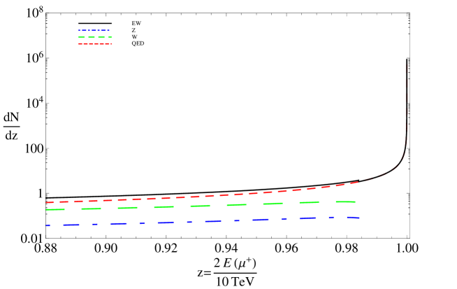
Figure 4: The same as Fig. 2 but zoomed in the region $z\approx 1$ and with the contributions coming from $\gamma$, $W$ and $Z$ emission drawn separately.

Let us now discuss which value one should give to $\Delta E$. In a collider, this value would be given by the (known) characteristics of the detector. Here however, the situation is less clear because of the effects of propagation from the interaction region to the point where the detector is physically placed. We choose to analyze two values for $\Delta E$. The first could be called the “optimal resolution case”: $\Delta E$ is chosen in such a way that the distribution (20) becomes a continuous line; in the case at hand this corresponds to $\Delta E\approx 0.3$ MeV. The resulting distribution for the positron is drawn in Fig. 2, where contributions from $\gamma$, $W$ and $Z$ radiation have been added together. Since the actual resolution on the positron energy is certainly worse than the “optimal” one, it is possible to obtain the actual distribution from the one in Fig. 2 simply by dividing it into “bins” of finite width. This is done in Fig. 3 where the more realistic case $\Delta E$= 30 GeV has been chosen. Finally, the region $z\approx 1$ from the “ideal case” in Fig. 2 is drawn for convenience in Fig. 4; here the contributions from $\gamma$, $Z$ and $W$ radiation are drawn separately.

Let us now discuss our results. In the first place, it is apparent from Fig. 4 that the emission of weak gauge bosons plays a significant role in determining the spectrum of the primary particle; therefore one should always consider QED ($\gamma$) and weak ($W$,$Z$) radiation together at very high energies. This is true even more so if the primary particle is an EW gauge boson itself instead of a fermion. In fact in this case QED radiation is partially suppressed because the gauge boson mass provides the collinear cutoff in Eq. (18), in place of the much smaller fermion mass considered here. Moreover, in the case of final EW gauge bosons since EW corrections of infrared origin are proportional to the Casimir of the external legs representations [5], they are expected to be bigger in magnitude.

We can see from Fig. 2 that even after inclusion of EW radiative corrections, the antifermion spectrum is rather sharply peaked at $z=1$. This can be seen also from Fig. 3, where the tree level distribution (dashed line) is also plotted for convenience. Virtual EW corrections deplete the first bin (from the right) by about 30 %, and produce therefore a significant effect. However the second bin is depressed with respect to the first one by 1-order of magnitude, and the others are even lower, so that the great majority of events falls into the first bin even after including radiative corrections.

4 Comparison with existing calculations

In [12] the effect of adding a weak gauge boson emission to a DM annihilation cross section at very high energies $\sqrt{s}\gg m_{W}$ was considered; in [14] a similar calculation for the case of very heavy decaying DM ($M\gg m_{W}$) was done. In both cases, corrections growing like the square of the c.m. energy were obtained. In particular, it was found that the cross section (width) with one additional gauge boson in the final state is obtained by multiplying the original one by a factor $R_{Z,W}(M)$:

$$R_{Z,W}(M)=\alpha_{W}K_{Z,W}\,\frac{M^{2}}{m_{W}^{2}}+...,$$ (21)

where $M$ is the relevant high energy scale ($\sqrt{s}$ in the case of scattering, DM mass in the case of decay), is supposed to be much higher than the weak scale; $K_{Z,W}$ is a constant that depends on whether a $Z$ or a $W$ is radiated. The dots here stand for terms that are subleading in the $M\gg m_{W}$ regime.

On the other hand, when integrated over the final gauge boson phase space (variable $x$), Eq. (14) gives

$$\frac{\Gamma_{3}(Z^{\prime}\rightarrow\bar{e}W^{-}\nu)}{\Gamma_{2}(Z^{\prime}\rightarrow e\bar{e})}=R_{W}(M)=\frac{\alpha_{W}}{8\pi}\left[\ln^{2}\frac{M^{2}}{4m_{W}^{2}}-3\ln\frac{M^{2}}{4m_{W}^{2}}+\ldots\right].$$ (22)

Similarly, virtual corrections described by (17) grow like the square of the logarithm of $M^{2}/m_{W}^{2}$. Our result therefore disagrees with the results obtained in [12, 13, 14], where corrections growing like $M^{2}/m_{W}^{2}$ were found. Here we wish to point out that the discrepancy is related to the introduction of dimension-4 operators that break $\mbox{SU}(2)_{L}\otimes\mbox{U}(1)_{Y}$ gauge invariance, and that one runs into ambiguous and possibly inconsistent results when trying to calculate virtual corrections in such framework.

Terms growing like $M^{2}/m_{W}^{2}$ are indeed present in the single contributions to the amplitude squared [see (9,11)] and are related to the terms in $k_{\mu}k_{\nu}/m_{W}^{2}$ in the sum over the emitted gauge boson polarizations. However, such terms are absent from the final result (22). This is a consequence of gauge symmetry in the form of Ward identities that are depicted in Fig. 5. These identities relate on shell amplitudes with an external gauge boson with corresponding amplitudes with an external Goldstone, in the following way:

$$\frac{k_{\mu}}{m_{W}}{\cal M}_{\mu}(k,...)=i{\cal M}(\varphi^{W}(k),...),$$ (23)

with $m_{W}$ being the mass of the relevant ($W$ or $Z$) gauge boson.
Since Goldstone bosons couple with fermions through their mass, the right-hand side is close to zero. Therefore the terms in the polarization sum proportional to $k_{\mu}k_{\nu}$, that are formally dominant by power counting with respect to the $g_{\mu\nu}$ term, are strongly suppressed at high energies.

A common feature of [12, 14] is the introduction in the Lagrangian of dimension-4 operators that explicitly break $\mbox{SU}(2)_{L}\otimes\mbox{U}(1)_{Y}$ gauge invariance: $D_{\mu}\overline{\nu_{L}}\gamma^{\mu}\nu_{L}$ and/or $D(\overline{\nu_{R}}\nu_{L}+\overline{\nu_{L}}\nu_{R})$ [to be compared with our gauge symmetry invariant Lagrangian in (1)]. Let us first consider real emissions.

Suppose that, following [12], we introduce a $D_{\mu}\overline{\nu_{L}}\gamma^{\mu}\nu_{L}$ interaction in the Lagrangian without its electron counterpart. Clearly, Ward identities are broken: for instance, from the point of view of our gauge invariant example, in the diagrams of Fig. 5   the second one on the left-hand side is missing. Then, the terms proportional to $M^{2}/m_{W}^{2}$ generated by the term proportional to $k_{\mu}k_{\nu}$ in the sum over polarizations do not cancel between the various contributions and are eventually present in the expression for the width. What one is really doing here is largely overestimating the contribution from longitudinal degrees of freedom, whose polarization is $\epsilon_{\mu}^{L}=\frac{k_{\mu}}{m_{W}}+O\left(\frac{m_{W}}{M}\right)$ and whose contribution, although leading by naive power counting with respect to transverse, is suppressed in a gauge invariant theory because of Ward identities.

As we have seen , virtual corrections have to be considered together with real emission for calculating the observed spectrum and, by virtue of (15), are important for unitarity of the theory. However we wish to point out that if, as done in [13], one calculates virtual corrections, the consistency of the calculation itself is put into doubt because, since Ward identities are broken, the final results will depend on the (arbitrary) gauge that one chooses in order to give a prescription for the weak gauge boson propagators. In fact the infrared structure is dominated by the region of phase space with on-shell gauge bosons. Since Ward identities are broken, the gauge dependent terms $\propto k_{\mu}k_{\nu}$ in the propagators are completely different, say, in the Feynman gauge and in the unitary gauge. These problems are generated by the exchange of soft quanta with energies greater than, but close to, the weak scale: therefore, we think that they cannot by cured by any “UV completion” beyond the TeV scale.

In Ref. [14], for phenomenological purposes, a chirality- (and gauge symmetry-)violating operator of the form $D(\overline{\nu_{R}}\nu_{L}+\overline{\nu_{L}}\nu_{R})$, with $D$ being a scalar and gauge singlet, is introduced into the Lagrangian. In this case only tree level gauge boson emissions have been considered. Notice that it is true that radiative corrections generate chirality violating terms proportional to the gauge symmetry breaking vacuum expectation value $v$ through fermion masses . However, since this term is generated in the framework of a gauge invariant theory (like the SM itself), Ward identities are obviously respected. On the contrary, by introducing a dimension-4 operator that explicitly violates gauge invariance, Ward identities are broken and by trying to compute radiative corrections one runs into the problems signaled above. One can, of course, write a gauge invariant interaction if the scalar DM particle is an isospin doublet: this would be similar to the usual Higgs-fermion-antifermion coupling in the standard model. We wish to point out that in this case, like in any other case where the DM particle has a weak charge, gauge boson emissions from the initial state have to be considered together with emissions from the final legs (see Fig. 6). If only final state radiation is considered, Ward identities are broken and one effectively breaks the $\mbox{SU}(2)_{L}\otimes\mbox{U}(1)_{Y}$ symmetry, potentially generating again “spurious” terms growing like the square of the energy.

One final comment: in our case the $Z^{\prime}$ can perfectly well couple to right neutrinos only, with the choice $f_{L}=f^{e}_{R}=0,f^{\nu}_{R}\neq 0$. The $Z^{\prime}$ then decays only into neutrinos and this situation, barring possible tiny chirality breaking effects proportional to fermion masses, is left unchanged by radiative corrections. Therefore, no final electrically charged states are present, even after including radiative corrections.

5 Conclusions

In this work we have analyzed the impact of radiative electroweak corrections on the spectrum of the final products resulting from the decay of a very heavy ($M>1$ TeV) weakly interacting particle. Determining accurately this spectrum is an important issue, in view of recent experimental results that can be interpreted as a dark matter signal. We have considered a simple model with a $Z^{\prime}$ gauge boson decaying into leptons, and rediscussed one loop radiative corrections plus emission of a weak gauge boson. We have found that electroweak corrections play a relevant role in this game; more precisely we can summarize our conclusions as follows:

• EW radiative corrections at one loop are of the order of 30 % in the considered case of fermions as primary particles, and grow like the log squared of the DM mass. One expects these corrections to be even bigger in the case of EW gauge bosons as primary particles (see Sec. 3); in any case, higher order effects play a significant role.

• QED corrections and “pure weak” corrections produced by $W$ and $Z$ exchange have a similar impact on the spectrum of the primary particle, so they should always be considered together.

• Different from recent results in the literature, we do not find corrections growing like the square of the energy. We have shown that the latter result can only be obtained if the Ward identities related to $\mbox{SU}(2)_{L}\otimes\mbox{U}(1)_{Y}$ gauge symmetry are broken. We have argued that this choice can lead to ambiguous results for virtual corrections and we think that this point should be better clarified in the future in view of its importance.

• As already noticed in [14], since EW corrections link all SM particles, all stable particles (including antiprotons) will be present in the final spectrum, independently of the primary particles (say, lepton/antileptons) initially considered.

• Heavy DM annihilation/decay can produce final states in which no electrically charged particles are present (see Sec. 4).

Let us now comment on the possible impact of EW corrections on indirect signals of dark matter. A detailed quantitative analysis including the effects of propagation goes beyond the scope of this work, but we can make some general comments. The first point is related to the fact that the $e^{\pm}$ excess measured in recent data in the 10 - 100 GeV region [6, 7, 8, 9] is not accompanied by a corresponding excess in the antiproton flux in the same energy region: the fraction $\frac{\bar{p}}{p}$ is indeed compatible with the astrophysical backgrounds [6]. One could then consider for instance DM annihilating to leptons only, or to $W^{+}W^{-}$ pairs with so high an invariant mass that the antiproton excess is shifted to energies higher than 100 GeV [19]. In both cases, however, taking into account EW corrections changes the scenario: in the first case allowing for final antiprotons coming from the decay of the weak gauge bosons irradiated by the leptons, and in the second case by softening the final gauge bosons spectrum. So radiative corrections of EW origin should be definitely taken in such kind of analyses.

Another issue is whether it is necessary, for the problem at hand, to consider higher order EW corrections. At first sight, one loop virtual corrections plus real gauge boson emission, as are done here, seem to be sufficient. In fact, as we have seen, one loop corrections are of the order of 30 % and higher order virtual corrections should not change the picture much: the experimental precision of the measurements involved is much lower than that of a earth based accelerator of course. However, this conclusion turns out to be a hasty one. In fact we are interested in the particles’ spectra, in the experimentally interesting region 10-100 GeV, produced by a decay annihilation taking place at a high invariant mass of the order of 1 TeV or more. Then, even if EW corrections on, say, the total cross section are relatively small, the impact on the spectrum at low energies can be dramatic, since “soft” ($\sim$ 10 GeV) particles are radiated copiously in the presence of a “hard “($\sim$ TeV) process. So one can determine whether or not higher order EW corrections are relevant in this context only after calculating their effects: this can and should be done in the future. Higher order EW radiative corrections and resummation of leading effects in the high energy regime have been extensively studied in recent years [3, 5]; recently a way of systematizing virtual corrections through soft collinear effective theory has been considered [20]. However, EW corrections are usually studied in two rather “extreme” cases: virtual corrections to a given hard process (in this case, $Z^{\prime}$ decay into a hard fermion and a hard antifermion) or the inclusive case where soft weak gauge boson emission is fully included. Determining the spectrum resulting from heavy DM annihilation/decay is a different, and difficult, case, where one wishes to know the distribution of a large number of particles in the final state. One possibility to deal with such a problem is to implement the EW evolution equations [16] (the analogous of the Dokshitzer-Gribov-Lipatov-Altarelli-Parisi equations in QCD) in parton shower Monte Carlo models. This seems to be unavoidable in the nearby future, especially if high energy lepton colliders [21], where showers generated by electroweakly charged particles will be ubiquitous, come closer to see the light.

6 Appendix: Kinematics

We consider the decay $Z^{\prime}(P)\rightarrow f(p_{1})\bar{f}(p_{2})$ with $P=(M,\mbox{\boldmath{$0$}})$, $p_{1}=(M/2,\mbox{\boldmath$p$})$, $p_{2}=(M/2,-\mbox{\boldmath$p$})$, and $p_{1,2}^{2}=m_{f}^{2}$. Then we consider the additional emission of a gauge boson with momentum $k$ and mass $\lambda$. The latter is parametrized in the following way:

$$k=(\omega,\mbox{\boldmath$k$}),\quad k^{2}=\lambda^{2};\qquad\qquad\mbox{\boldmath$p$}\cdot\mbox{\boldmath$k$}=|\mbox{\boldmath$p$}||\mbox{\boldmath$k$}|\cos\theta;$$ (24)

We consider the region where the emitted boson is collinear to $\mbox{\boldmath$p$}_{1}=\mbox{\boldmath$p$}$ so that $\theta\ll 1$ (the region where $k$ is collinear to $\mbox{\boldmath$p$}_{2}=-\mbox{\boldmath$p$}$ can be treated in a similar way). In our calculations the following expression appears:

$$\frac{d^{3}\overrightarrow{k}}{(2\pi)^{3}2\omega}\frac{2p_{1}\cdot p_{2}}{[(p_{1}+k)^{2}-m_{f}^{2}][(p_{2}+k)^{2}-m_{f}^{2}]}\,,$$ (25)

where the differential phase space is evaluated in the collinear region to give

$$\frac{d^{3}\overrightarrow{k}}{(2\pi)^{3}2\omega}=\frac{\omega}{(4\pi)^{2}}d\omega d\theta^{2}.$$ (26)

The denominator appearing in (25) is evaluated differently in the case of QED ($\lambda=0$) and in the case of weak gauge bosons emission ($\lambda=m_{W}\gg m_{f}$).

In the case of QED we have

$$(p_{2}+k)^{2}-m_{f}^{2}=2p_{2}\cdot k\approx 2M\omega,\qquad(p_{1}+k)^{2}-m_{f}^{2}=2p_{1}\cdot k\approx\frac{M\omega}{2}(\theta^{2}+\frac{4m_{f}^{2}}{M^{2}}),$$ (27)

and the integration over $\theta^{2}$ readily produces

$$\frac{d^{3}\overrightarrow{k}}{(2\pi)^{3}2\omega}\frac{2p_{1}\cdot p_{2}}{[(p_{1}+k)^{2}-m_{f}^{2}][(p_{2}+k)^{2}-m_{f}^{2}]}=\frac{dx}{x}\frac{1}{16\pi^{2}}\ln\frac{M^{2}}{4m_{f}^{2}},$$ (28)

where $x=2\omega/M$ is the fraction of energy carried away by the emitted photon.

In the case of weak gauge boson emission we have

$$(p_{2}+k)^{2}-m_{f}^{2}=m_{W}^{2}+2p_{2}\cdot k\approx 2M\omega,\qquad(p_{1}+k)^{2}-m_{f}^{2}=2p_{1}\cdot k+m_{W}^{2}\approx\frac{M\omega}{2}(\theta^{2}+\frac{m_{W}^{2}}{\omega^{2}}),$$ (29)

and integrating over $\theta^{2}$:

$$\frac{d^{3}\overrightarrow{k}}{(2\pi)^{3}2\omega}\frac{2p_{1}\cdot p_{2}}{[(p_{1}+k)^{2}-m_{f}^{2}][(p_{2}+k)^{2}-m_{f}^{2}]}=\frac{dx}{x}\frac{1}{16\pi^{2}}\ln\frac{M^{2}x^{2}}{4m_{W}^{2}}.$$ (30)

Figure 2: Spectrum $\frac{dN}{dz}$ of the primary particle (antimuon) coming from the decay of a heavy $Z^{\prime}$ ($M=10$ TeV) after inclusion of one loop virtual corrections and EW gauge bosons emission. Here and in the following figures z$=2E/M$, with $E$ being the antimuon energy. An “optimal resolution” is assumed (see text).

Figure 3: Continuous line: the same as Fig. 2 but with an experimental resolution $\Delta E(\mu)=30$ GeV. Dashed line: tree level distribution with no electroweak corrections.

Figure 5: Ward identity relevant for the process considered in this paper.

Figure 6: Gauge boson emission diagrams (the wavy line is a $Z$ or a $W$) for the case of a heavy scalar decaying into a fermion or an antifermion.

References

- [1] J. H. Kuhn, A. Kulesza, S. Pozzorini and M. Schulze, Nucl. Phys. B 797 (2008) 27.
- [2] P. Ciafaloni and D. Comelli, Phys. Lett. B 446 (1999) 278.
- [3] M. Ciafaloni, P. Ciafaloni and D. Comelli, Phys. Rev. Lett. 84, 4810 (2000); Nucl.Phys. B 589 359 (2000); Phys. Lett. B 501, 216 (2001); Phys. Rev. Lett. 87 (2001) 211802; Nucl. Phys. B 613 (2001) 382; Phys. Rev. Lett. 88, 102001 (2002); JHEP 0805 (2008) 039; P. Ciafaloni, D. Comelli and A. Vergine, JHEP 0407, 039 (2004); M. Ciafaloni, Lect. Notes Phys. 737 (2008) 151; P. Ciafaloni and D. Comelli, JHEP 0511 (2005) 022.
- [4] V. S. Fadin, L. N. Lipatov, A. D. Martin and M. Melles, Phys. Rev. D 61 (2000) 094002; P. Ciafaloni, D. Comelli, Phys. Lett. B 476 (2000) 49; J. H. Kuhn, A. A. Penin and V. A. Smirnov, Eur. Phys. J. C 17, 97 (2000); J. H. Kuhn, S. Moch, A. A. Penin, V. A. Smirnov, Nucl. Phys. B 616, 286 (2001) [Erratum-ibid. B 648, 455 (2003)]; M. Melles, Phys. Rept. 375, 219 (2003); J. y. Chiu, F. Golf, R. Kelley and A. V. Manohar, Phys. Rev. D 77 (2008) 053004.
- [5] A. Denner, S. Dittmaier and T. Hahn, Phys. Rev. D 56, 117 (1997); A. Denner and T. Hahn, Nucl. Phys. B 525, 27 (1998); M. Beccaria, G. Montagna, F. Piccinini, F. M. Renard and C. Verzegnassi, Phys. Rev. D 58 (1998) 093014; P. Ciafaloni and D. Comelli, Phys. Lett. B 446, 278 (1999); V. S. Fadin, L. N. Lipatov, A. D. Martin and M. Melles, Phys. Rev. D 61 (2000) 094002; P. Ciafaloni, D. Comelli, Phys. Lett. B 476 (2000) 49; J. H. Kuhn, A. A. Penin and V. A. Smirnov, Eur. Phys. J. C 17, 97 (2000); J. H. Kuhn, S. Moch, A. A. Penin, V. A. Smirnov, Nucl. Phys. B 616, 286 (2001) [Erratum-ibid. B 648, 455 (2003)]; M. Melles, Phys. Rept. 375, 219 (2003); J. H. Kuhn, A. Kulesza, S. Pozzorini and M. Schulze, Phys. Lett. B 609 (2005) 277 A. Denner, B. Jantzen and S. Pozzorini, Nucl. Phys. B 761 (2007) 1; J. H. Kuhn, A. Kulesza, S. Pozzorini and M. Schulze, E. Accomando, A. Denner and S. Pozzorini, JHEP 0703 (2007) 078; Nucl. Phys. B 797 (2008) 27; J. y. Chiu,F. Golf, R. Kelley and A. V. Manohar, Phys. Rev. D 77 (2008) 053004; J. y. Chiu, R. Kelley and A. V. Manohar, Phys. Rev. D 78 (2008) 073006; A. Denner, B. Jantzen and S. Pozzorini, JHEP 0811 (2008) 062; P. Ciafaloni and A. Urbano, Phys. Rev. D 81 (2010) 085033; P. Ciafaloni and D. Comelli, JHEP 0609, 055 (2006).
- [6] O. Adriani et al. [PAMELA Collaboration], Nature 458 (2009) 607; Phys. Rev. Lett. 102, 051101 (2009).
- [7] A. A. Abdo et al. [The Fermi LAT Collaboration], Phys. Rev. Lett. 102, 181101 (2009).
- [8] J. Chang et al., Nature 456, 362 (2008).
- [9] F. Aharonian et al. [H.E.S.S. Collaboration], Phys. Rev. Lett. 101 (2008) 261104.
- [10] M. Papucci and A. Strumia, JCAP 1003, 014 (2010); M. Cirelli, M. Kadastik, M. Raidal and A. Strumia, Nucl. Phys. B 813 (2009) 1.
- [11] http://home.thep.lu.se/~torbjorn/Pythia.html
- [12] N. F. Bell, J. B. Dent, T. D. Jacques and T. J. Weiler, Phys. Rev. D 78 (2008) 083540.
- [13] J. B. Dent, R. J. Scherrer and T. J. Weiler, Phys. Rev. D 78 (2008) 063509.
- [14] M. Kachelriess, P. D. Serpico and M. A. Solberg, Phys. Rev. D 80, 123533 (2009).
- [15] M. Melles, Phys. Rept. 375 (2003) 219.
- [16] M. Ciafaloni, P. Ciafaloni and D. Comelli, Phys. Rev. Lett. 88 (2002) 102001; P. Ciafaloni and D. Comelli, JHEP 0511, 022 (2005).
- [17] M. Kachelriess and P. D. Serpico, Phys. Rev. D 76 (2007) 063516.
- [18] M. Ciafaloni, P. Ciafaloni and D. Comelli, JHEP 1003, 072 (2010).
- [19] A. Strumia, Prog. Theor. Phys. Suppl. 180, 128 (2009).
- [20] J. y. Chiu, A. Fuhrer, R. Kelley and A. V. Manohar, Phys. Rev. D 81, 014023 (2010); Phys. Rev. D 80 (2009) 094013; J. y. Chiu, A. Fuhrer, A. H. Hoang, R. Kelley and A. V. Manohar, PoS E FT09, 009 (2009); J. y. Chiu, R. Kelley and A. V. Manohar, Phys. Rev. D 78 (2008) 073006; J. y. Chiu, F. Golf, R. Kelley and A. V. Manohar, Phys. Rev. D 77 (2008) 053004.
- [21] For perspectives on future high energy lepton colliders see for instance Fermilab’s muon collider homepage http://www.fnal.gov/pub/muon_collider/index.html, the International Linear Collider homepage http://www.linearcollider.org/cms/ and the Compact LInear Collider homepage http://clic-study.web.cern.ch/clic-study/