A periodic orbit formula for quantum reactions through transition states

Abstract

Transition State Theory forms the basis of computing reaction rates in chemical and other systems. Recently it has been shown how transition state theory can rigorously be realized in phase space using an explicit algorithm. The quantization has been demonstrated to lead to an efficient procedure to compute cumulative reaction probabilities and the associated Gamov-Siegert resonances. In this letter these results are used to express the cumulative reaction probability as an absolutely convergent sum over periodic orbits contained in the transition state.

Introduction.— Transition State Theory, developed by Eyring, Polanyi and Wigner in the 1930’s, is the most fundamental and widely used method to compute reaction rates. During a reaction a molecular system is envisaged to pass through a ‘transition state’ or ‘activated complex’, a kind of unstable supermolecule poised between reactants and products Pechukas (1981). The main idea of transition state theory is to place a dividing surface in the transition state region and compute the classical reaction rate from the directional flux through the dividing surface. In order not to overestimate the reaction rate the dividing surface needs to have the crucial property that it is crossed exactly once by all reactive trajectories (trajectories passing from reactants to products or vice versa) and not crossed at all by all other (non-reactive) trajectories. In the 1970’s Pechukas, Pollak and others showed how to rigorously construct such a dividing surface from a periodic orbit giving the so-called periodic orbit dividing surface (PODS) Pechukas and McLafferty (1973). The generalization to more degrees of freedoms has posed a major problem, and was solved only recently using ideas from dynamical systems theory (see Wiggins et al. (2001)). This shows that the transition state at energy $E$ is formed by a normally hyperbolic invariant manifold (NHIM) (see Wiggins (1994)), which in this case is an invariant sphere of dimension $2d-3$, where $d$ is the number of degrees of freedoms, and normal hyperbolicity means that the contraction and expansion rates associated with the directions normal to the sphere dominate those of the directions tangential to the sphere. For $d=2$, this simply is the unstable periodic orbit of the PODS Waalkens and Wiggins (2004). In fact, the NHIM spans another sphere which is of dimension $2d-2$ and hence has one dimension less than the energy surface and can be taken as a dividing surface. The NHIM forms the equator of this sphere and divides it into one hemisphere crossed exactly once by all forward reactive trajectories and one hemisphere crossed exactly once by all backward reactive trajectories. The NHIM itself is invariant and can be viewed as the energy surface of an invariant subsystem (the ‘transition state’ or ‘activated complex’) with one degree of freedom less than the full system (i.e. with the reaction coordinate being frozen at a particular value). All these phase space structures can be explicitly constructed from a normal form which at the same time gives a simple expression for the flux through the dividing surface. In Schubert et al. (2006) the quantization of this normal form has been used to develop a quantum version of transition state theory. This quantum normal form has been demonstrated to give an efficient method to compute cumulative reaction probabilities (the quantum analogue of the classical flux) and Gamov-Siegert resonances associated with the activated complex Schubert et al. (2006); Goussev et al. (2009). In this letter we use these results to show that the cumulative reaction probability can be expressed as a sum over periodic orbits contained in the activated complex.

The normal form representation of the activated complex and the computation of reaction rates.— We consider a molecular system with $d=1+f$ degrees of freedom which has a saddle-center-…-center equilibrium point (‘saddle’ for short), i.e. the matrix associated with the linearized Hamilton’s equations has one pair of real eigenvalues $\pm\lambda$, and $f$ pairs of purely imaginary eigenvalues $\pm\mathrm{i}\omega_{k}$, $k=1,\ldots,f$. We will restrict ourselves to the generic case of linear frequencies $\omega_{k}$ fulfilling no resonance condition $m_{1}\omega_{1}+\ldots+m_{f}\omega_{f}=0$ for any vector of integers ${\mathbf{m}}=(m_{1},\ldots,m_{f})\neq 0$. Such saddles are characteristic for reaction type dynamics as for energies near the energy of the saddle, they induce a bottleneck type structure of the energy surface near the saddle through which the system has to pass in order to react.

Normal form theory shows that in the neighborhood of the saddle there is a canonical transformation such that the transformed Hamiltonian is of the form $H_{0}(I,J_{1},\ldots,J_{f})$, where $I=(p_{0}^{2}-q_{0}^{2})/2$ is an integral associated with the reaction coordinate, and the $J_{k}=(p_{k}^{2}+q_{k}^{2})/2$, $k=1,\ldots,f$, are action integrals associated with the bath modes. The activated complex is the invariant subsystem given by $p_{0}=q_{0}=0$. Its motions are described by the reduced Hamiltonian $H_{0}(0,J_{1},\ldots,J_{f})$, and thus is integrable, i.e. in action angle variables $({\mathbf{J}},\bm{\varphi})$ the equations of motion are $\dot{{\mathbf{J}}}=0$ and ${\dot{\bm{\varphi}}}=\nabla_{\mathbf{J}}H_{0}(0,{\mathbf{J}})$ with solutions ${\mathbf{J}}(t)=const$ and

$$\bm{\varphi}(t)=\bm{\varphi}_{0}+t\,{\bm{\Omega}}({\mathbf{J}})\text{ mod }2\pi\,,\,\text{where}\,\,{\bm{\Omega}}({\mathbf{J}}):=\nabla_{{\mathbf{J}}}H_{0}(0,{\mathbf{J}})\,\,.$$ (1)

The motion is thus quasiperiodic. It takes place on invariant $f$ dimensional Liouville-Arnold tori Arnold (1978) which foliate the phase space of the activated complex. The motion becomes periodic for the ${\mathbf{J}}$ for which ${\bm{\Omega}}({\mathbf{J}})=a{\mathbf{m}}$, where ${\mathbf{m}}\in\mathds{Z}^{f}$ and $a\in\mathds{R}$. We call the torus corresponding to this ${\mathbf{J}}$ a resonant torus. Fixing the energy $E$ the energy surface of the activated complex,

$$\Sigma_{E}=\{{\mathbf{J}}\in\mathds{R}^{f}_{+}\,:\,H_{0}(0,J_{1},\ldots,J_{f})=E\}\,,$$ (2)

is the action space projection of the NHIM mentioned in the introduction. The volume it encloses in the space of the actions ${\mathbf{J}}$ is proportional to the directional flux through the dividing surface (see Fig. 1).

A quantum normal form procedure based on the Weyl symbol calculus Schubert et al. (2006) shows that in the quantum mechanical case a unitary transformation can be found which transforms the Hamilton operator to the form $\hat{H}=H(\hat{I},\hat{J}_{1},\ldots,\hat{J}_{n})$ which is a polynomial function of the operators $\hat{I}=(-\hbar^{2}\partial_{q_{1}}^{2}-q_{1}^{2})/2$ and $\hat{J}_{k}=(-\hbar^{2}\partial_{q_{k}}^{2}+q_{k}^{2})/2$ associated with the classical integrals. The polynomial defining the quantum normal form operator has the $\hbar$ expansion $H(I,{\mathbf{J}})=H_{0}(I,{\mathbf{J}})+\hbar H_{1}(I,{\mathbf{J}})+\ldots$, where $H_{k}(I,{\mathbf{J}})$ are independent of $\hbar$, and $H_{0}(I,{\mathbf{J}})$ coincides with the classical normal form Hamiltonian.

The cumulative reaction probability at energy $E$ is then given by

$$N(E)=\sum_{{\bf n}\in\mathds{N}_{0}^{f}}\frac{1}{1+\mathrm{e}^{-2\pi I_{\bf n}/\hbar}}\,,$$ (3)

where $I_{\mathbf{n}}=I_{\mathbf{n}}(E)$ is implicitly defined by

$$H(I_{\bf n},J_{1},\ldots,J_{f})=E\,,$$ (4)

and ${\mathbf{n}}=(n_{1},\ldots,n_{f})\in\mathds{N}_{0}^{f}$ is the vector of quantum numbers for the Bohr-Sommerfeld quantized actions,

$$J_{k}=\hbar(n_{k}+\frac{\alpha_{k}}{2})\,,\quad k=1,\ldots,f\,.$$ (5)

Here the $\alpha_{k}=2$ are Maslov indices which for later reference we group in the vector ${\bm{\alpha}}=(\alpha_{1},\ldots,\alpha_{f})$ (see Miller (1977) for an earlier reference and Schubert et al. (2006) where this result is derived in a systematic semiclassical expansion in $\hbar$). In the following we derive a formula which expresses $N(E)$ in terms of a sum over periodic orbits.

A periodic orbit formula for the cumulative reaction probability.— To derive our periodic orbit formula it is convenient to consider the energy derivative of the cumulative reaction probability (3),

$$n(E):=\frac{\mathrm{d}N(E)}{\mathrm{d}E}=\sum_{{\bf n}\in\mathds{N}_{0}^{f}}\frac{2\pi}{\hbar}\frac{\mathrm{d}I_{n}}{\mathrm{d}E}\frac{1}{4\cosh^{2}(\pi I_{\mathbf{n}}/\hbar)}\,.$$ (6)

Using (4) the factor $\mathrm{d}I_{n}/\mathrm{d}E$ can be written as

$$\frac{\mathrm{d}I_{\mathbf{n}}}{\mathrm{d}E}=\left.\frac{\partial H}{\partial I}\right|_{I=I_{\mathbf{n}},J_{k}=\hbar(n_{k}+\frac{1}{2})}^{-1}\,.$$ (7)

We can obtain a periodic orbit formula for $n(E)$ following a computation similar to the derivation of the Berry-Tabor trace formula for the density of states of classically integrable systems Berry and Tabor (1976). Following Berry and Tabor (1976) we use the Poisson summation formula to rewrite (6) as

$$\begin{split}n(E)=&\sum_{{{\mathbf{m}}}\in\mathds{Z}^{f}}n_{\bf m}(E):=\sum_{{\bf m}\in\mathds{Z}^{f}}\frac{2\pi}{\hbar^{f+1}}\mathrm{e}^{-\mathrm{i}\pi{\bm{\alpha}}{\mathbf{m}}/2}\times\\ &\int\mathrm{d}^{f}J\left.\frac{\partial H}{\partial I}\right|_{I=I(E,{\mathbf{J}})}^{-1}\frac{1}{4\cosh^{2}(\pi I(E,{\mathbf{J}})/\hbar)}\mathrm{e}^{2\pi\mathrm{i}{\bf m}\cdot{\bf J}/\hbar}\,,\end{split}$$ (8)

where $I(E,{\mathbf{J}})$ is determined by

$$H(I(E,{\mathbf{J}}),J_{1},\ldots,J_{f})=E\,.$$ (9)

Note that the $\hbar$ expansion of the quantum normal form Hamiltonian implies, via (9), an $\hbar$ expansion of $I(E,{\mathbf{J}})$, i.e. $I(E,{\mathbf{J}})=I_{0}(E,{\mathbf{J}})+\hbar I_{1}(E,{\mathbf{J}})+\ldots$. In the following we separately discuss the term $n_{0}$ which we refer to as the Thomas-Fermi term Berry and Tabor (1976), and the remaining sum over ${\mathbf{m}}\neq 0$ which we refer to as the oscillatory term $n_{\text{osc}}(E)$.

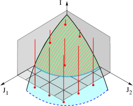
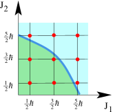
Figure 1: For $d=3$ degrees of freedom, the left panel shows an energy surface $H_{0}(I,J_{2},J_{3})=E$ for an energy above the saddle energy. The red lines mark the Bohr-Sommerfeld quantized actions ${\mathbf{J}}$. The right panel shows the energy surface of the activated complex $\Sigma_{E}$ defined in (2) marked as the blue line in the left panel. The enclosed area is proportional to the classical flux, and equivalently, to the mean number of states of the activated complex.

The Thomas-Fermi term.— For ${\bf m}=0$, we get

$$n_{0}(E)=\frac{2\pi}{\hbar^{f+1}}\int\mathrm{d}^{f}J\left.\frac{\partial H}{\partial I}\right|_{I=I(E,{\mathbf{J}})}^{-1}\frac{1}{4\cosh^{2}(\pi I(E,{\mathbf{J}})/\hbar)}\,.$$ (10)

This term can easily be interpreted from considering its integrated version

$$N_{0}(E)=\int^{E}_{-\infty}\mathrm{d}E^{\prime}\,n_{0}(E^{\prime})=\frac{1}{\hbar^{f}}\int\mathrm{d}^{f}J\frac{1}{1+\mathrm{e}^{-2\pi I(E,{\mathbf{J}})/\hbar}}\,.$$ (11)

In the semiclassical limit, $\hbar\to 0$, the integrand can be viewed as a characteristic function on the action space region $I(E,{\mathbf{J}})>0$. The integral in (11) hence gives the action space volume enclosed by the surface $I(E,{\mathbf{J}})=0$, and accordingly $N_{0}(E)$ is given by the classical flux divided by the elementary volume $(2\pi\hbar)^{f}$, which agrees with the mean number of states of the activated complex to energy $E$ Schubert et al. (2006) (see Fig. 1). The term $n_{0}(E)$ is the corresponding differential version, i.e. the mean density of states of the activated complex at energy $E$.

The oscillatory term.— To compute the terms $n_{\bf m}(E)$ for ${\bf m}\neq 0$ we use Prudnikov et al. (1986)

$$\frac{1}{4\cosh^{2}(\pi x)}=\frac{1}{(2\pi)^{2}}\int_{-\infty}^{\infty}\mathrm{d}y\frac{y/2}{\sinh(y/2)}\mathrm{e}^{-\mathrm{i}yx}$$ (12)

to rewrite (8) as

$$\begin{split}n_{{\mathbf{m}}}(E)=\frac{\mathrm{e}^{-\mathrm{i}\pi{\mathbf{m}}{\bm{\alpha}}/2}}{2\pi\hbar^{f+1}}&\int\mathrm{d}y\int_{J\geq 0}\mathrm{d}^{f}J\bigg{(}\frac{\partial H}{\partial I}\bigg{)}^{-1}_{I(E,{\mathbf{J}})}\times\\ &\frac{y/2}{\sinh(y/2)}\mathrm{e}^{\mathrm{i}[2\pi{\mathbf{m}}{\mathbf{J}}-yI({\mathbf{J}},E)]/\hbar}\,.\end{split}$$ (13)

This integral can be evaluated by the method of stationary phase. The stationary phase conditions are

$$2\pi{\mathbf{m}}=y\nabla_{J}I_{0}(E,{\mathbf{J}})\,\,,\qquad I_{0}(E,{\mathbf{J}})=0\,,$$ (14)

and by differentiating $H_{0}(I_{0}(E,{\mathbf{J}}),{\mathbf{J}})=E$ we obtain

$$2\pi{\mathbf{m}}=-\frac{y}{\lambda({\mathbf{J}})}{\bm{\Omega}}({\mathbf{J}})\,\,,\quad\text{where}\quad\lambda({\mathbf{J}}):=\frac{\partial H_{0}}{\partial I}(0,{\mathbf{J}})\,.$$ (15)

The second condition in (14) restricts ${\mathbf{J}}$ to the energy surface of the activated complex $\Sigma_{E}$ defined in (2). The first conditions then fixes a point ${\mathbf{J}}_{{\mathbf{m}}}$ on $\Sigma_{E}$ (or a finite number of points ${\mathbf{J}}_{{\mathbf{m}},i}$) by requiring that the frequency vector ${\bm{\Omega}}({\mathbf{J}})$ at ${\mathbf{J}}_{{\mathbf{m}}}$ is proportional to ${\mathbf{m}}$. By (1) this means that the torus corresponding to ${\mathbf{J}}_{{\mathbf{m}}}$ is resonant, and by (15) we have

$$\lvert y\rvert=2\pi\frac{\lambda}{\lvert{\bm{\Omega}}\rvert}\lvert{\mathbf{m}}\rvert\,,$$ (16)

where $y<0$ ($y>0$) if ${\mathbf{m}}$ and ${\bm{\Omega}}$ are parallel (anti-parallel). Here all functions of ${\mathbf{J}}$ are evaluated at ${\mathbf{J}}_{{\mathbf{m}}}$. Let $Q$ be the $(f+1)\times(f+1)$ matrix of second derivatives of the phase function in (13) evaluated at ${\mathbf{J}}_{{\mathbf{m}}}$ and $y$, and $\beta$ its signature. We then find for $n_{{\mathbf{m}}}(E)$,

$$\frac{(2\pi)^{\frac{f-1}{2}}\mathrm{e}^{-\mathrm{i}[\pi{\mathbf{m}}{\bm{\alpha}}/2+2\pi\lvert{\mathbf{m}}\rvert\lambda I_{1}/\lvert{\bm{\Omega}}\rvert+\pi\beta/4]}}{\hbar^{\frac{f+1}{2}}\lambda\sqrt{\lvert\det Q\rvert}}\frac{y/2}{\sinh(y/2)}\mathrm{e}^{2\pi\mathrm{i}{\mathbf{m}}{\mathbf{J}}_{{\mathbf{m}}}/\hbar}\,.$$ (17)

To evaluate the determinant of $Q$ it is useful to introduce the curvature tensor $K$ of $\Sigma_{E}$. Let $\mathbf{e}_{1},\mathbf{e}_{2},\ldots,\mathbf{e}_{f-1}$ be $f-1$ orthogonal unit vectors which are tangent to $\Sigma_{E}$ at ${\mathbf{J}}$. Noting that $\Sigma_{E}$ is the hypersurface $I_{0}(E,{\mathbf{J}})=0$ we can write the components of $K$ at ${\mathbf{J}}_{\mathbf{m}}$ as

$$K_{ij}=-\frac{1}{\lvert\nabla_{\mathbf{J}}I_{0}\rvert}\mathbf{e}_{i}\cdot I_{0}^{\prime\prime}\mathbf{e}_{j}=-\frac{1}{\lvert\nabla_{\mathbf{J}}H_{0}\rvert}\mathbf{e}_{i}\cdot H_{0}^{\prime\prime}\mathbf{e}_{j}\,,$$ (18)

where $I_{0}^{{}^{\prime\prime}}$ and $H_{0}^{\prime\prime}$ denote the matrices of second derivatives with respect to ${\mathbf{J}}$. Let $\mathbf{e}_{1}$ be the unit vector parallel to $\nabla_{\mathbf{J}}H_{0}={\bm{\Omega}}$. Then in the basis of the $\mathbf{e}_{j}$ the matrix $Q$ becomes

$$Q=\begin{pmatrix}0&\lvert{\bm{\Omega}}\rvert/\lambda&0^{T}\\ \lvert{\bm{\Omega}}\rvert/\lambda&-y\mathbf{e}_{1}I_{0}^{\prime\prime}\mathbf{e}_{1}&\mathbf{a}^{T}\\ 0&\mathbf{a}&y\lvert\nabla_{\mathbf{J}}I_{0}\rvert K\end{pmatrix}\,\,,$$ (19)

where $\mathbf{a}$ has components $\mathbf{e}_{1}I_{0}^{\prime\prime}\mathbf{e}_{j}$. The determinant of this matrix can be evaluated straightforwardly, but to determine as well the signature it is useful to rewrite it as follows. Let $A$ be the upper left $2\times 2$ block of (19), $D=y\lvert\nabla I_{0}\rvert K$ and $B=\begin{pmatrix}0&\mathbf{a}\end{pmatrix}$, then if $\det K\neq 0$ we can form

$$\begin{pmatrix}A&B^{T}\\ B&D\end{pmatrix}=\begin{pmatrix}I&B^{T}D^{-1}\\ 0&I\end{pmatrix}\begin{pmatrix}A-B^{T}D^{-1}B&0\\ 0&D\end{pmatrix}\begin{pmatrix}I&0\\ D^{-1}B&I\end{pmatrix}\,.$$

By the special structure of $B$ we find that $B^{T}D^{-1}B=\begin{pmatrix}0&0\\ 0&c\end{pmatrix}$ for some number $c$. Hence $\det(A-B^{T}D^{-1}B)=-\lvert{\bm{\Omega}}\rvert^{2}/\lambda^{2}<0$ and so $A-B^{T}D^{-1}B$ has signature $0$. The signature $\beta$ of $Q$ is thus determined by $D=y\lvert\nabla_{\mathbf{J}}I_{0}\rvert K$ and we find

$$\beta=\operatorname{sign}y\operatorname{sign}K\,\,,$$ (20)

and with $y\nabla_{\mathbf{J}}I_{0}=2\pi{\mathbf{m}}$, by (14), the determinant is

$$\sqrt{\lvert\det Q\rvert}=(2\pi\lvert{\mathbf{m}}\rvert)^{\frac{f-1}{2}}\sqrt{\lvert\det K\rvert}\,\lvert{\bm{\Omega}}\rvert/\lambda$$

evaluated at ${\mathbf{J}}={\mathbf{J}}_{{\mathbf{m}}}$.

We notice that if ${\mathbf{J}}_{{\mathbf{m}}}$ and $y$ are a solution to the stationary phase condition for ${\mathbf{m}}$, then ${\mathbf{J}}_{{\mathbf{m}}}$ and $qy$ are a solution for $q{\mathbf{m}}$ for any $q\in\mathds{Z}\backslash\{0\}$. It is natural to choose ${\bm{\mu}}\sim{\mathbf{m}}$ with positive coprime components and combine the two terms with $q{\bm{\mu}}$ and $-q{\bm{\mu}}$. This way the $n(E)$ contribution of the $q\text{th}$ repetition of a resonant torus with ${\bm{\Omega}}\sim{\bm{\mu}}$ is given by

$$\begin{split}&n_{{\bm{\mu}},q}(E)=\frac{2\pi}{\hbar^{(f+1)/2}}\frac{\lambda}{\sinh\big{(}\pi q\frac{|{\bm{\mu}}|}{|{\bm{\Omega}}|}\lambda\big{)}}\times\\ &\frac{\cos\big{(}q(2\pi{\bm{\mu}}\cdot{\mathbf{J}}/\hbar-\pi{\bm{\mu}}{\bm{\alpha}}/2-2\pi\lvert{\bm{\mu}}\rvert\lambda I_{1}/\lvert{\bm{\Omega}}\rvert)+\pi\beta/4\big{)}}{q^{(f-3)/2}|{\bm{\mu}}|^{(f-3)/2}|{\bm{\Omega}}|^{2}\sqrt{|\det K({\mathbf{J}}^{\bm{\mu}})|}}\,.\end{split}$$ (21)

Example.— We consider the example of a system composed of an Eckart barrier and two Morse oscillators. Its quantum normal form Hamiltonian is given by Schubert et al. (2006)

$$\hat{H}=(\frac{\pi}{a_{0}}\sqrt{\frac{V_{0}}{2m}}+\hat{I})^{2}-\sum_{k=1}^{2}(\sqrt{D_{k}}-\frac{a_{k}}{\sqrt{2m}}\hat{J}_{k})^{2}\,.$$ (22)

Here $H=H_{0}$, and hence $I_{1}=0$. The frequencies are

$$\Omega_{k}=\partial_{J_{k}}H_{0}=a_{k}\sqrt{\frac{2D_{k}}{m}}-\frac{a_{k}^{2}}{m}J_{k}\,,\quad k=1,2\,,$$ (23)

and

$$\lambda=\left.\frac{\partial H_{0}}{\partial I}\right|_{I=0}=\frac{2\pi}{a_{0}}\sqrt{\frac{V_{0}}{2m}}\,.$$ (24)

We choose $D_{2}=a_{1}=a_{2}=1$, $D_{1}=5/6$, $a_{0}=4\pi$, $V_{0}=5/4$, and $\hbar=0.1$. Figure 2 shows energy surfaces $\Sigma_{E}$ of the activated complex consisting of the two Morse oscillators together with some resonance lines $\Omega_{1}/\Omega_{2}=\mu_{1}/\mu_{2}$. The sign of the curvature matrix is $\beta=-1$. The exact cumulative reaction probability, and its derivative $n(E)$ can be computed analytically for this system Schubert et al. (2006). Its oscillatory part, $n_{\text{osc}}=n(E)-n_{0}(E)$, is shown together with its approximation by the periodic orbit sum over the terms (21) for $\mu_{1},\mu_{2}\leq 3$ in Fig. 3.

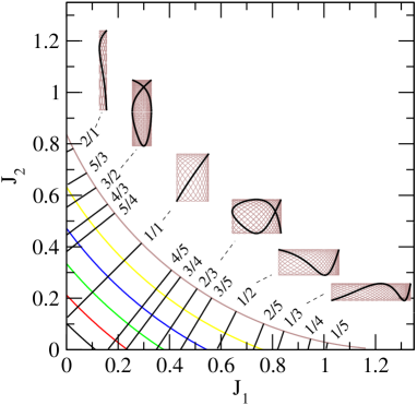
Figure 2: Energy surfaces with resonance lines $\mu_{1}/\mu_{2}$ of the activated complex which consists of two Morse oscillators. The insets show the resonant tori with $\mu_{1},\mu_{2}\leq 3$ projected to the configuration space of the oscillators.

Figure 3: Exact (dashed line) and periodic orbit approximation (solid line) of the energy derivative of the cumulative reaction probability including resonant tori with $\mu_{1},\mu_{2}\leq 3$.

Conclusions.— In this letter we derived a periodic orbit formula for the cumulative reaction probability, and demonstrated its applicability for a simple example. In the limit $\lambda\to 0$ (no tunneling through the potential barrier) our periodic orbit formula reduces to the Berry-Tabor trace formula for the density of states of the activated complex. In the general case $\lambda\neq 0$, our periodic orbit formula is (as opposed to the Berry-Tabor trace formula) absolutely convergent due to an additional factor which leads to an exponential damping of contributions of long periodic orbits. Although we incorporated only six periodic obits (and their repetitions) in our example the agreement with the exact result is already very good. This is even more impressive as we have so far only taken into account simple stationary points associated with resonant tori, and no isolated and ghost orbits which would naturally arise in a more elaborate uniform approximation Berry and Tabor (1976); Richens (1982). Similarly, the integral associated with the reaction direction can be cast into a periodic orbit sum over the instanton orbits Miller (1977) extending the applicability of our periodic orbit formula to energies below the saddle energy. These aspects will be discussed in more detail in a longer version of this letter.

Acknowledgments.— This work was supported by EPSRC under Grant No. EP/E024629/1 and ONR under Grant No. N00014-01-1-0769.

References

Pechukas (1981)
P. Pechukas,
Ann. Rev. Phys. Chem. 32,
159 (1981).
Pechukas and McLafferty (1973)
P. Pechukas and
F. J. McLafferty,
J. Chem. Phys. 58,
1622 (1973);
P. Pechukas and
E. Pollak,
J. Chem. Phys. 69,
1218 (1978).
Wiggins et al. (2001)
S. Wiggins,
L. Wiesenfeld,
C. Jaffé,
and T. Uzer,
Phys. Rev. Lett. 86,
5478 (2001);
T. Uzer,
C. Jaffé,
J. Palacián,
P. Yanguas, and
S. Wiggins,
Nonlinearity 15,
957 (2001).
Wiggins (1994)
S. Wiggins,
Normally Hyperbolic Invariant Manifolds in
Dynamical Systems (Springer,
Berlin, 1994).
Waalkens and Wiggins (2004)
H. Waalkens and
S. Wiggins,
J. Phys. A 37,
L435 (2004).
Schubert et al. (2006)
R. Schubert,
H. Waalkens, and
S. Wiggins,
Phys. Rev. Lett. 96,
218302 (2006);
H. Waalkens,
R. Schubert, and
S. Wiggins,
Nonlinearity 21,
R1 (2008).
Goussev et al. (2009)
A. Goussev,
R. Schubert,
H. Waalkens, and
S. Wiggins,
J. Chem. Phys. 131,
144103 (2009).
Arnold (1978)
V. I. Arnold,
Mathematical Methods of Classical Mechanics,
vol. 60 of Graduate Texts in
Mathematics (Springer, Berlin,
1978).
Miller (1977)
W. H. Miller,
Faraday Discussions 62,
40 (1977).
Berry and Tabor (1976)
M. V. Berry and
M. Tabor,
Proc. R. Soc. Lond. A 349,
101 (1976).
Prudnikov et al. (1986)
A. Prudnikov,
B. Y.A., and
O. Marichev,
Integrals & Series Vol. I
(Gordon & Breach Science Publishers,
London, 1986).
Richens (1982)
P. J. Richens,
J. Phys. A: Math. Gen. 15,
2101 (1982).