Nitrogen chemistry and depletion in starless cores

Abstract

Aims. We investigated the chemistry of nitrogen–containing species, principally isotopomers of CN, HCN, and HNC, in a sample of pre-protostellar cores.

Methods. We used the IRAM 30 m telescope to measure the emission in rotational and hyperfine transitions of CN, HCN, ${\rm{}^{13}CN}$, H${\rm{}^{13}CN}$, HN${\rm{}^{13}C}$, and HC${\rm{}^{15}N}$ in L 1544, L 183, Oph D, L 1517B, L 310. The observations were made along axial cuts through the dust emission peak, at a number of regularly–spaced offset positions. The observations were reduced and analyzed to obtain the column densities, using the measurements of the less abundant isotopic variants in order to minimize the consequences of finite optical depths in the lines. The observations were compared with the predictions of a free–fall gravitational collapse model, which incorporates a non-equilibrium treatment of the relevant chemistry.

Results. We found that CN, HCN, and HNC remain present in the gas phase at densities well above that at which CO depletes on to grains. The CN:HCN and the HNC:HCN abundance ratios are larger than unity in all the objects of our sample. Furthermore, there is no observational evidence for large variations of these ratios with increasing offset from the dust emission peak and hence with density. Whilst the differential freeze–out of CN and CO can be understood in terms of the current chemistry, the behaviour of the CN:HCN ratio is more difficult to explain. Models suggest that most nitrogen is not in the gas phase but may be locked in ices. Unambiguous conclusions require measurements of the rate coefficients of the key neutral–neutral reactions at low temperatures.

1 Introduction

Table 1: The sample of cores observed. Note that $\rho$Oph D is also known as L 1696A.

Source	$\alpha_{2000}$	$\delta_{2000}$	$\Delta\alpha,\Delta\delta^{a}$	$v_{{\rm LSR}}^{b}$	$n({\rm H_{2}})^{c}$	$S_{1.2\rm mm}$	$N({\rm H_{2}})^{d}$	$T_{{\rm kin}}^{e}$	References
			′′	${\rm km\,s^{-1}}$	${\rm 10^{5}}$ ${\rm cm^{-3}}$	${{\rm MJy\,sr^{-1}}}$	${\rm 10^{22}}$${\rm cm^{-2}}$	K
L 183	15:54:08.80	-02:52:44.0	$(0,0)$	2.37	20	18.3	7.2	7.0	(1)
L 1544	05:04:16.90	+25:10:47.0	$(0,0)$	7.20	14	17.2	6.7	7.0	(2)
Oph D	16:28:30.40	-24:18:29.0	$(0,0)$	3.35	8.5	14.6	5.7	6.0	(3)
L 1517B	04:55:18.80	+30:38:03.8	$(-10,-20)$	5.87	2.2	7.1	2.8	10.0	(4)
L 310	18:07:11.90	-18:21:35.0	$(30,80)$	6.70	0.9	7.5	2.9	9.0	(5)

• ^a Offsets of the continuum peak with respect to the reference position.

• ^b Systemic LSR velocity.

• ^c Peak particle number density.

• ^d Column density computed assuming $T_{\rm dust}=8$ K and $\kappa_{\nu}=0.01\rm\,cm^{2}g^{-1}$. The values increase by 25% if $T_{\rm dust}=7$ K.

• ^e Gas kinetic temperature from the literature.

• (1) Pagani et al. (2004, 2007), (2) Tafalla et al. (2002), Crapsi et al. (2007), (3) Ward-Thompson et al. (1999), Harju et al. (2008) (4) Tafalla et al. (2004) (5) Bacmann et al. (2002)

Observations of rotational transitions of molecules and radicals play a key role in deriving information on solar–mass objects in the early stages of gravitational collapse. The variation of the intensities of the emission lines can be interpreted in terms of the chemical reactions and gas–grain interactions occurring in the medium, and the line profiles and frequency shifts in terms of the kinematics of the collapsing gaseous material. Indeed, apart from infrared observations of dust continuum emission, which yield no chemical or kinematical information, measurements of radio transitions of molecules provide the only means of probing the evolution of pre-protostellar cores.

An obstacle to the use of molecular line emission to study the early stages of star formation is the propensity of some molecules to freeze on to the grains at the low temperatures, $T\approx 10$ K, which prevail. Observations of prestellar cores have shown that the fractional abundances of the carbon–containing species, CO and CS, decrease strongly towards the core centres, whereas the fractions of the nitrogen–containing species, ${\rm N_{2}H^{+}}$ and NH₃, either remain constant or even increase towards the centre, where the density is highest (Tafalla et al. 2002). Differential freeze–out of the C- and N-containing species on to the grains was the generally–accepted explanation of these observational results. However, recent observations of the NO radical have demonstrated that the real situation is more complicated. A comparison of the profiles of NO and ${\rm N_{2}H^{+}}$ along cuts through the prestellar cores L 1544 and L 183 (Akyilmaz et al. 2007, hereafter A07) has shown that the fractional abundance of NO, unlike that of ${\rm N_{2}H^{+}}$, decreases towards the centres of these cores (their centres being identified with the peak of the dust emission). Thus, not all nitrogen–containing species remain in the gas phase at densities $\gtrsim{\rm 10^{6}}$ ${\rm cm^{-3}}$, which prevail in the central regions. On the other hand, still more recent observations of CN (Hily-Blant et al. 2008) have shown that the emission of this radical follows closely the dust emission in both L 1544 and L 183. In so far as these two objects are representative of their class, it appears that the adsorption process must somehow differentiate between nitrogen–bearing species.

In the present work, we extended our observations of nitrogen–containing species to include isotopomers of HCN. In addition to L 1544 and L 183, we have studied Oph D, L 1517B, and L 310. The observations are described and analyzed in Section 2. Sections 3 and 4 describe the observations and present estimates of N-bearing species abundances. In Section 5, we consider the chemical processes, including freeze–out on to the grains, which determine the gas–phase abundances of key N– and also C– and O–containing species in prestellar cores. Section 6 summarizes the model that has been adopted of the early stages of the collapse of the representative prestellar core L 1544. The fractional chemical abundances predicted by the model are presented and the corresponding column density profiles are compared with the observations. Finally, in Section 7, we make our concluding remarks.

2 Observational procedures and data reduction

The observations were performed at the IRAM 30 m telescope in January 2008. The data have been reduced and anlayzed using the CLASS90 software (Hily-Blant et al. 2005). The instrumental setup was identical to that used by Hily-Blant et al. (2008): frequency–switching spectra, with a frequency-throw of 7.8 MHz, were recorded by the VESPA facility, with 20 kHz spectral resolution and 20 to 80 MHz bandwidth. The half-power beam-width is calculated as HPBW$[^{\scriptscriptstyle\prime\prime}]=2460/\nu[\rm GHz]$, that is 28^′′ at 87 GHz and 22^′′ at 113 GHz. Cross–like patterns with 20^′′ spacing were observed towards each source. The crosses were centered on the dust emission peak, as determined from published continuum maps; all offsets quoted in the present paper refer to the central positions listed in Table LABEL:tab:cores. Table 5 summarizes the lines observed for each object. The amplitude calibration was checked every 10 min, the pointing every hour, and the focus every two hours, typically. Instrumental spectral effects were compensated by subtracting polynomial baselines from each spectrum before folding. More details on the data reduction procedures can be found in Appendix B. All results (unless explicitly stated) have been translated from the antenna temperature scale ($T_{{\rm A}}^{*}$) to the main-beam temperature scale $T_{{\rm mb}}=T_{{\rm A}}^{*}\times F_{{\rm{eff}}}/B_{{\rm{eff}}}$, with the values of $B_{{\rm{eff}}}$ listed in Table 5; $F_{{\rm{eff}}}$ is the forward efficiency, and $B_{{\rm{eff}}}$ is the beam efficiency.

Figure 1: Continuum emission (${{\rm MJy\,sr^{-1}}}$) at 1.2mm with the locations of the line integrations (crosses). The HPBW at 1.2 mm and at the 3 mm frequencies discussed in this paper are indicated. A linear scale of 0.05 pc is also shown, assuming a distance of 150 pc for all cores except L 183 (110 pc). Continuum maps for L 1544, Oph D, L 183, L 1517B and L 310 are taken from Ward-Thompson et al. (1999), Pagani et al. (2003), Tafalla et al. (2004) and Bacmann et al. (2000) respectively.

3 Observational results

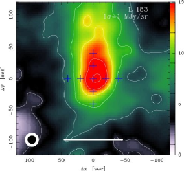
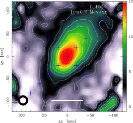
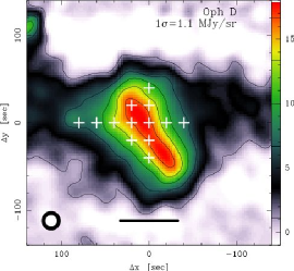
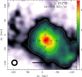
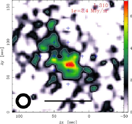
All objects in our sample are pre-stellar, in the sense that none shows signposts of embedded stellar objects. Their peak particle number densities span more than an order of magnitude (see Table LABEL:tab:cores): the peak densities decrease from approximately ${\rm 10^{6}}$ ${\rm cm^{-3}}$ (L 183, L 1544) to $0.9{\times 10^{5}}$ ${\rm cm^{-3}}$ in L 310. All the objects have been extensively observed, both in their lines and continuum (see Fig. 1). Our observations focused on the nitrogen–bearing species CN, HCN, ${\rm{}^{13}CN}$, H${\rm{}^{13}CN}$, HN${\rm{}^{13}C}$, and HC${\rm{}^{15}N}$. All these molecules present hyperfine structure (HFS). However, in the cases of HN${\rm{}^{13}C}$ and HC${\rm{}^{15}N}$, the hyperfine structures were not resolved in our 20 kHz resolution spectra. All transitions are in the 3 mm band; the CN$(2-1)$ line was observed in parallel at 1.3 mm (see Table 4).

3.1 Line properties

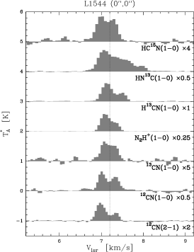
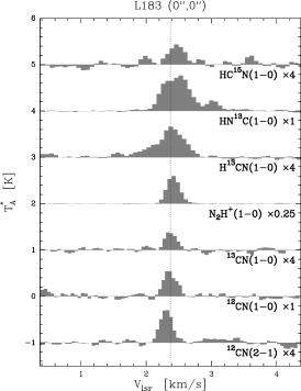
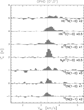
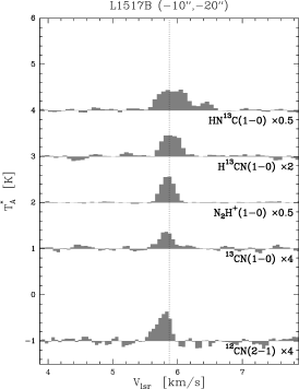
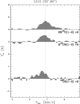
All lines were observed successfully towards the three most centrally peaked cores, L 183, L 1544, and Oph D; the emission lines are shown in Fig. 2. For CN and ${\rm N_{2}H^{+}}$$(1-0)$, only the weakest HFS components (at 113520.4315 MHz and 93176.2650 MHz) are shown. For each of the other lines, the strongest HFS component is considered instead: 108780.2010 MHz, 86340.1840 MHz, 87090.8590 MHz, and 86054.9664 MHz for ${\rm{}^{13}CN}$$(1-0)$, H${\rm{}^{13}CN}$, HN${\rm{}^{13}C}$ and ${\rm HC{\rm{}^{15}N}}$$(1-0)$ respectively. The HN${\rm{}^{13}C}$ hyperfine structure is not fully resolved and the two hyperfine transitions of ${\rm HC{\rm{}^{15}N}}$ are not resolved. The ${\rm{}^{13}CN}$ line is detected in the four densest objects, L 183, L 1544, Oph D and L 1517B.

Tables 6-10 give the properties of all lines towards all the positions in each source. The integrated intensities, $W$, were derived from Gaussian fitting of a given HFS component (see above). Several Gaussian components were fitted in some cases, e.g. for the known hyperfine structure of HN${\rm{}^{13}C}$, and also in the obvious cases of multiple–component line profiles (L 1544). In such cases, $W$ is the sum of the integrated intensities of each velocity component. The peak temperature $T_{\rm mb}$ is the maximum intensity over the line. Given that the lines are, in general, not Gaussian, the linewidth is estimated as the equivalent width, $\Delta v=W/T_{\rm mb}$ and the statistical uncertainty is obtained by propagating the errors. For non-detections, upper limits on the integrated intensity were obtained by fitting a Gaussian at a fixed position. Upper limits on the intensity are at the 3$\sigma$ level while those on the integrated intensity are at the 5$\sigma$ level.

Towards L 1544, all resolved lines show two clear peaks, with a dip centred at 7.20 ${\rm km\,s^{-1}}$. These two peaks are seen in several tracers including ${\rm H^{13}CO^{+}}$ by Hirota et al. (2003) who concluded that there are two distinct velocity components along the line of sight (Tafalla et al. 1998). Owing to their double–peak profiles, lines towards L 1544 have the largest integrated intensities of all the lines that we observed.

The comparison of the ${\rm{}^{13}CN}$ linewidths shows that the lines towards L 183 are the narrowest with full widths at half maximum (FWHM) $\approx 0.20$ ${\rm km\,s^{-1}}$. The H${\rm{}^{13}CN}$ line in this source exhibits a blue wing and the profile can be well fitted by two Gaussian components with FWHM of 0.38 and 0.85 ${\rm km\,s^{-1}}$; this blue wing is not evident in any other tracer. Towards Oph D and L 1517B, the linewidth is larger by a factor of 2 to 3, although the comparison with L 1544 is rendered difficult by the double–peak line profiles. In several tracers, e.g. H${\rm{}^{13}CN}$, L 310 displays the largest linewidth ($<0.8$ ${\rm km\,s^{-1}}$) but small integrated intensities. In all the sources, ${\rm HC{\rm{}^{15}N}}$ has been detected, and the properties of the line, averaged over all offset positions, are listed in Table 2. The peak and integrated intensities decrease as the peak density decreases. Again, L 1544 seems to be an exception, owing to the double–peak line profile. The FWHM are comparable ($\approx 0.4\leavevmode\nobreak\ {\rm km\,s^{-1}}$) for all sources; but, once again, the FWHM is significantly larger (by a factor 2) in L 310 than in the other sources.

Table 2: Properties of the average ${\rm HC{\rm{}^{15}N}}$$(1-0)$ profiles and average fractional abundance towards the observed cores (main beam temperature scale).

Source	$\langle T_{{\rm mb}}\rangle$	$\langle W\rangle$	$\langle v_{0}\rangle$	$\langle\rm FWHM\rangle$	$\langle N({\rm HC{\rm{}^{15}N}})\rangle$	$\langle N({\rm H_{2}})\rangle_{20^{\scriptscriptstyle\prime\prime}}\,^{b}$	$\langle N\rangle/\langle 2N({\rm H_{2}})\rangle\,^{d}$
	mK	m${\rm K\,km\,s^{-1}}$	${\rm km\,s^{-1}}$	${\rm km\,s^{-1}}$	${\times 10^{10}}$ ${\rm cm^{-2}}$	${\times 10^{22}}$ ${\rm cm^{-2}}$	$\times{\rm 10^{-12}}$
L 183	125 $\pm$ 15	47 $\pm$ 4	2.49	0.35 $\pm$ 0.04	8.9$\pm$0.8	5.6	0.8
L 1544a	170 $\pm$ 12	85 $\pm$ 5	7.20	0.48 $\pm$ 0.05	16.1$\pm$1.0	4.3	1.9
Oph D	102 $\pm$ 15	47 $\pm$ 6	3.44	0.43 $\pm$ 0.08	8.9$\pm$1.1	5.6	0.8
L 1517B	82 $\pm$ 15	29 $\pm$ 3	5.69	0.33 $\pm$ 0.04	5.5$\pm$0.6	2.0	1.4
L 310	20 $\pm$ 10	21 $\pm$ 3	6.69	0.98 $\pm$ 0.16	4.0$\pm$0.6	0.8	2.5

• ^a Using a two–component Gaussian fit. The FWHM is taken to be the equivalent linewidth, in this case; $v_{0}=7.2$ ${\rm km\,s^{-1}}$ is adopted from Hily-Blant et al. (2008).

• ^b Column density of ${\rm H_{2}}$ derived from the dust emission smoothed to 20^′′, assuming $T_{\rm dust}=8$ K (see Table LABEL:tab:cores). The total (statistical and systematic) uncertainty is 30%.

• ^d The uncertainty is typically 40%.

3.2 Line ratios

The ratios of total integrated intensities $W_{\rm tot}$ for some line combinations in each source, are shown in Fig. 9. Under the optically thin assumption, these ratios reflect the relative abundances. The ratios CN/HCN or ${\rm{}^{13}CN}$/H${\rm{}^{13}CN}$ are constant to within a factor of 2 across all the cores and vary between about 0.5 to 5 from source to source. Towards L 1517B, the ${\rm{}^{13}CN}$/H${\rm{}^{13}CN}$ ratio appears to decrease towards the centre. Significant also is the fact that the H${\rm{}^{13}CN}$/HN${\rm{}^{13}C}$ is constant and of similar magnitude (0.2–0.8) in all sources, independent of the central density.

Most of the lines that have been observed are split by the hyperfine interaction, and the relative intensities of the hyperfine components can be used as a measure of optical depth. It is generally assumed that the level populations of hyperfine states are in LTE and hence proportional to the statistical weights, within a given rotational level. However, it has been known for some time that this assumption is often invalid (see, for example, the discussion of Walmsley et al. 1982), and this is confirmed by our data. When the populations are in LTE, one expects the satellite line intensity ratios to lie between the ratios of the line strengths, in the optically thin limit, and unity for high optical depths. As may be seen from Fig. 3, this is usually but not always the case. For example, it is clear that the CN$(1-0)$ ratios towards L 183 are inconsistent with this expectation, whereas the ratios observed towards other sources suggest high optical depths and are broadly consistent with equal excitation temperatures in the different components. The observed ${\rm{}^{13}CN}$ ratios show clear signs of deviations from LTE, but the effects are much less drastic than in the more abundant isotopomer, and we suspect that optical depths are low. In the case of H${\rm{}^{13}CN}$, departures from LTE appear to be minor.

The reasons for departures from LTE such as seen in Fig. 3 are presently unknown and need to be established. Such an investigation would require calculations of the collisional rate coefficients, analogous to those of Monteiro & Stutzki (1986), as well as a treatment of the radiative transfer; this is beyond the scope of the current study. For the present, we use low abundance isotopomers such as ${\rm{}^{13}CN}$ and H${\rm{}^{13}CN}$ to trace abundance gradients, neglecting collisional excitation and the possibility of fractionation of the ¹³C and ¹⁵N isotopomers.

Table 3: Fractional abundances of CN, HCN, HNC and ${\rm N_{2}H^{+}}$ relative to H towards the dust emission peaks of our source sample. Tables 6–10 give the fractional abundances toward all the observed positions.

Source	[CN]	[HCN]	[HNC]	[${\rm N_{2}H^{+}}$]	[NO]a	CN:HCN	HNC:HCN
	${\times 10^{-9}}$	${\times 10^{-9}}$	${\times 10^{-9}}$	${\times 10^{-10}}$	${\times 10^{-9}}$
L 183	0.40	0.17	0.45	0.78	10.0	2.4	2.6
L 1544	1.11	0.56	1.12	1.20	4.0	2.0	2.0
Oph D	0.37	0.23	0.38			1.6	1.7
L 1517B	1.12	0.48	1.50			2.3	3.1
L 310	4.40	1.50	2.50			2.9	1.6

• $\rm[X]=n(X)/2n({\rm H_{2}})$. An isotopic ratio ${\rm{}^{12}C}:{\rm{}^{13}C}=68$ was assumed when using the ${\rm{}^{13}C}$ isotopologues.

• A global uncertainty (including statistical and systematic errors) of 40% is assumed.

• ^a The abundance of NO is taken from A07.

Figure 2: Comparison of the line profiles of different tracers; the spectra have been shifted vertically for clarity. For CN$(1-0)$, $(2-1)$, and ${\rm N_{2}H^{+}}$$(1-0)$, the weakest HFS components (at 113520.4315, 226887.3520 and 93176.2650 MHz respectively) are shown. For each of the other lines, the strongest HFS component is considered: 108780.2010, 86340.1840, 87090.8590, and 86054.9664 MHz for ${\rm{}^{13}CN}$$(1-0)$, H${\rm{}^{13}CN}$, HN${\rm{}^{13}C}$ and ${\rm HC{\rm{}^{15}N}}$$(1-0)$ respectively. The ${\rm N_{2}H^{+}}$ spectrum is taken from A07. The spectra are for zero offset (cf. Table LABEL:tab:cores). Towards L 1517B, the CN$(1-0)$ spectrum is replaced by CN$(2-1)$ and the ${\rm N_{2}H^{+}}$ spectrum is taken from Tafalla et al. (2002). Towards Oph D, the ${\rm N_{2}H^{+}}$ spectrum at offset (0^′′, 0^′′) is taken from Crapsi et al. (2005).

Figure 3: Relative integrated intensity of each HFS component for several species, at the central position for each source. In each panel, the dashed line indicates the relative intensities in LTE for optically thin emission. The thick line shows the optically thick limit. The abscissa is the rest line frequency.

Figure 4: Derived column densities towards each source. From top to bottom: L 1544, L 183, Oph D, and L 1517B. The column densities are plotted as a function of the distance from the dust emission peak, along both cuts. Also plotted is the H₂ column density (grey histogram, right scale), as derived from the dust emission (assuming $T_{\rm dust}=8$ K and $\kappa=0.01\,\rm cm^{2}\,g^{-1}$). The right panels show the corresponding abundances.

Figure 5: Same as Fig. 4 for the derived fractional abundances.

4 Column densities and abundance ratios

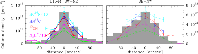
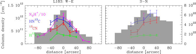
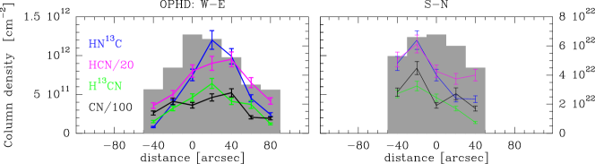
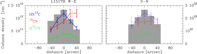
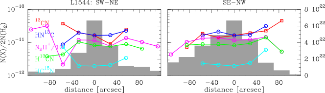
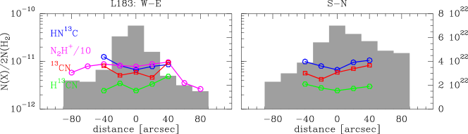
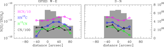
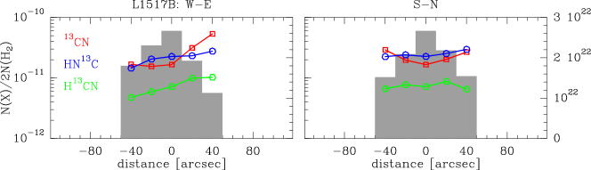
We determine column densities using the standard formalism described in Appendix C (Eq. 23 and 24) and assume the local (solar neighbourhood) $\rm{}^{12}C:^{13}$C$=68$ ratio. It is instructive to consider also the abundance variations from source to source. Converting column densities into relative abundances requires the molecular hydrogen column density, $N_{{\rm H_{2}}}$, which we have determined (indirectly) from measurements of the dust emission, using bolometer maps available in the literature (Ward-Thompson et al. 1999; Pagani et al. 2003; Tafalla et al. 2004; Bacmann et al. 2000) and smoothing where necessary to a 20^′′ beam. We assumed a dust temperature of 8 K and a 1.3 mm absorption coefficient of $\kappa=0.01\leavevmode\nobreak\ \rm cm^{2}\,g^{-1}$ (see HWFP08). The results are shown in Fig. 5 for L1544, L 183, Oph D, and L 1517B.

We remark first that, towards L 1544 , the column densities of ${\rm{}^{13}CN}$, H${\rm{}^{13}CN}$, and ${\rm HN{\rm{}^{13}C}}$ are all roughly proportional to the hydrogen column density, as inferred from dust emission (see Fig. 4); this has been noted already by HWPF08 for the case of ${\rm{}^{13}CN}$. The derived abundances do not change appreciably towards the dust peak, in spite of a variation of almost an order of magnitude in the hydrogen column density. Thus, in this source, and with the current resolution, the CN–containing species do not appear to be significantly depleted at high densities. On the other hand, the abundances tend to increase to the NW of the dust emission peak (see the SE–NW cut); we assume that this is related to asymmetry of the source. It is interesting that ${\rm N_{2}H^{+}}$ behaves in similar fashion. Important for the later discussion is the fact that the abundance ratios ${\rm HN{\rm{}^{13}C}}$:H${\rm{}^{13}CN}$ and ${\rm{}^{13}CN}$:H${\rm{}^{13}CN}$ are approximately equal to 2 (with variations of up to a factor of 2); we assume that this reflects the ratios HNC:HCN and CN:HCN, respectively.

However, L 1544 is not typical. Towards L 183, for example (see the EW cuts in Fig. 4), the peak H${\rm{}^{13}CN}$ and ${\rm HN{\rm{}^{13}C}}$ column densities are offset to the east, relative to the dust emission, whereas ${\rm N_{2}H^{+}}$ and ${\rm{}^{13}CN}$ appear to follow the dust emission. The situation is similar in Oph D although we did not observe ${\rm{}^{13}CN}$ in this source. Towards L 1517B, ${\rm HN{\rm{}^{13}C}}$ correlates reasonably well with $N({\rm H_{2}})$ but this is not the case of ${\rm{}^{13}CN}$ nor, probably, of H${\rm{}^{13}CN}$. Bearing in mind the inaccuracy of the abundance determinations, and the possibility of ¹³C fractionation, we conclude conservatively that there is no evidence for an order of magnitude variation in the CN:HCN nor the HNC:HCN abundance ratios between the dust emission peak and offset positions.

We give also in Table 3 our estimates of the fractional abundances, relative to H, of CN, HCN, and HNC towards the dust emission peaks of our sample of sources; these abundances have been derived assuming the local value of 68 for the ¹²C:¹³C ratio. All the relative abundances are of order ${\rm 10^{-9}}$, with CN and HNC being more abundant than HCN by a factor of about 2. This value is close to the ratio determined by Irvine & Schloerb (1984) toward TMC-1. Values larger than 1 for the HNC:HCN abundance ratio were found towards a sample of 19 dark clouds by Hirota et al. (1998) with an average ratio of $2.1\pm 1.2$. We do not see indications of significant abundance differences between cores of high central density (L 1544 and L 183) and cores of lower central density (L 1517B, Oph D). Whilst the complexities of the source structure and of radiation transfer prevent our establishing the existence of small abundance differences, we may conclude that there remain appreciable amounts of CN, HCN, and HNC at densities above the typical density (3${\times 10^{4}}$ ${\rm cm^{-3}}$) at which CO depletes on to grains. Not surprisingly, this effect is seen most readily in sources of high central column density, like L 1544, in which emission from the low density envelope is less important.

5 Chemical considerations

In this Section, we seek to update and extend previous studies of the interstellar chemistry of N–containing species Pineau des Forêts et al. (1990); Schilke et al. (1992), with a view to providing a framework for the interpretation of our observations of prestellar cores. We shall show that it is possible to derive a simple expression for the CN:HCN abundance ratio, in particular, by identifying the principal reactions involved in the formation and destruction of these species.

5.1 Main chemical reactions

The fractional abundances of gas–phase species in prestellar cores are determined by:

• the initial composition of the molecular gas which undergoes gravitational collapse;

• variations of the density with time;

• the rates of gas–phase reactions at the low temperatures ($T\approx 10$ K) of the cores;

• the rates of adsorption of the constituents of the gas on to grains.

The assumption of steady state, when computing the initial abundances, is not crucial when dealing with species which are produced in ion–neutral reactions. The timescales associated with ion–neutral reactions are much smaller, in general, than dynamical timescales, notably the gravitational free–fall time. Consequently, the evolution of the fractional abundances of species which are formed in such reactions soon becomes independent of the initial values. However, it is believed that the timescales for producing N–containing species, such as NH₃ and CN, are determined by slower neutral–neutral reactions. It follows that their fractional abundances in the subsequent gravitational collapse may depend significantly on the initial values.

The conversion of atomic into molecular nitrogen in the gas phase is believed to occur in the reactions

$${{{{\mathrm{\mathrm{N}}}}+{}{{\mathrm{\mathrm{OH}}}}{{}\xrightarrow[]{\hskip 10.00002pt}{}}{{\mathrm{\mathrm{NO}}}}+{}{{\mathrm{\mathrm{H}}}}}}$$ (1)

$${{{{\mathrm{\mathrm{N}}}}+{}{{\mathrm{\mathrm{NO}}}}{{}\xrightarrow[]{\hskip 10.00002pt}{}}{{\mathrm{\mathrm{N}}_{\vphantom{\mathrm{}}\mathrm{2}}^{\vphantom{\mathrm{}}\vphantom{\mathrm{\smash[t]{2+}}}\mathrm{}}}}+{}{{\mathrm{\mathrm{O}}}}}}$$ (2)

and

$${{{{\mathrm{\mathrm{N}}}}+{}{{\mathrm{\mathrm{CH}}}}{{}\xrightarrow[]{\hskip 10.00002pt}{}}{{\mathrm{\mathrm{CN}}}}+{}{{\mathrm{\mathrm{H}}}}}}$$ (3)

$${{{{\mathrm{\mathrm{N}}}}+{}{{\mathrm{\mathrm{CN}}}}{{}\xrightarrow[]{\hskip 10.00002pt}{}}{{\mathrm{\mathrm{N}}_{\vphantom{\mathrm{}}\mathrm{2}}^{\vphantom{\mathrm{}}\vphantom{\mathrm{\smash[t]{2+}}}\mathrm{}}}}+{}{{\mathrm{\mathrm{C}}}}}}$$ (4)

The reactions

$${{{{\mathrm{\mathrm{C}}}}+{}{{\mathrm{\mathrm{NO}}}}{{}\xrightarrow[]{\hskip 10.00002pt}{}}{{\mathrm{\mathrm{CN}}}}+{}{{\mathrm{\mathrm{O}}}}}}$$ (5)

$${{{{\mathrm{\mathrm{C}}}}+{}{{\mathrm{\mathrm{NO}}}}{{}\xrightarrow[]{\hskip 10.00002pt}{}}{{\mathrm{\mathrm{CO}}}}+{}{{\mathrm{\mathrm{N}}}}}}$$ (6)

can also destroy NO, producing CN in the case of (5), and

$${{{{\mathrm{\mathrm{CN}}}}+{}{{\mathrm{\mathrm{O}}}}{{}\xrightarrow[]{\hskip 10.00002pt}{}}{{\mathrm{\mathrm{CO}}}}+{}{{\mathrm{\mathrm{N}}}}}}$$ (7)

can destroy CN.

From the above, we see that NO forms from the reaction of N with OH, whereas CN forms from N and CH. It follows that the ratio of carbon to oxygen in the gas phase is a factor determining the relative abundance of NO and CN. The NO:CN abundance ratio will be lower in gas which is depleted of oxygen, either because of an intrinsically high C:O elemental abundance ratio, or due to the differential freeze–out of O and C on to the grains, where the oxygen is incorporated mainly as water ice.

Once N₂ has formed, in (2) and (4), N₂H⁺ is produced in the protonation reaction

$${{{{\mathrm{\mathrm{N}}_{\vphantom{\mathrm{}}\mathrm{2}}^{\vphantom{\mathrm{}}\vphantom{\mathrm{\smash[t]{2+}}}\mathrm{}}}}+{}{{\mathrm{\mathrm{H}}_{\vphantom{\mathrm{}}\mathrm{3}}^{\vphantom{\mathrm{}}\vphantom{\mathrm{\smash[t]{2+}}}\mathrm{+}}}}{{}\xrightarrow[]{\hskip 10.00002pt}{}}{{\mathrm{\mathrm{N}}_{\vphantom{\mathrm{}}\mathrm{2}}^{\vphantom{\mathrm{}}\vphantom{\mathrm{\smash[t]{2+}}}\mathrm{}}\nolinebreak\mathrm{\mathrm{H}}_{\vphantom{\mathrm{}}\mathrm{}}^{\vphantom{\mathrm{}}\vphantom{\mathrm{\smash[t]{2+}}}\mathrm{+}}}}+{}{{\mathrm{\mathrm{H}}_{\vphantom{\mathrm{}}\mathrm{2}}^{\vphantom{\mathrm{}}\vphantom{\mathrm{\smash[t]{2+}}}\mathrm{}}}}}}$$ (8)

Dissociative ionization of N₂ by He⁺ results in the production of N⁺:

$${{{{\mathrm{\mathrm{N}}_{\vphantom{\mathrm{}}\mathrm{2}}^{\vphantom{\mathrm{}}\vphantom{\mathrm{\smash[t]{2+}}}\mathrm{}}}}+{}{{\mathrm{\mathrm{He}}_{\vphantom{\mathrm{}}\mathrm{}}^{\vphantom{\mathrm{}}\vphantom{\mathrm{\smash[t]{2+}}}\mathrm{+}}}}{{}\xrightarrow[]{\hskip 10.00002pt}{}}{{\mathrm{\mathrm{N}}_{\vphantom{\mathrm{}}\mathrm{}}^{\vphantom{\mathrm{}}\vphantom{\mathrm{\smash[t]{2+}}}\mathrm{+}}}}+{}{{\mathrm{\mathrm{N}}}}+{}{{\mathrm{\mathrm{He}}}}}}$$ (9)

Whilst the reaction of N⁺ with para–H₂ (in its ground rotational state) is endothermic, by approximately 168 K, its reaction with ortho–H₂ is slightly exothermic and occurs even at low temperatures Le Bourlot (1991). Subsequent hydrogenation reactions with H₂ lead to NH${}_{4}^{+}$, which can dissociatively recombine to produce NH₃. Thus, N₂ is a progenitor of both N₂H⁺ and NH₃, whilst NO and CN are intermediaries in the formation of N₂.

HCN and HNC are produced principally in the reactions

$${{{{\mathrm{\mathrm{CH}}_{\vphantom{\mathrm{}}\mathrm{2}}^{\vphantom{\mathrm{}}\vphantom{\mathrm{\smash[t]{2+}}}\mathrm{}}}}+{}{{\mathrm{\mathrm{N}}}}{{}\xrightarrow[]{\hskip 10.00002pt}{}}{{\mathrm{\mathrm{HCN}}}}+{}{{\mathrm{\mathrm{H}}}}}}$$ (10)

$${{{{\mathrm{\mathrm{NH}}_{\vphantom{\mathrm{}}\mathrm{2}}^{\vphantom{\mathrm{}}\vphantom{\mathrm{\smash[t]{2+}}}\mathrm{}}}}+{}{{\mathrm{\mathrm{C}}}}{{}\xrightarrow[]{\hskip 10.00002pt}{}}{{\mathrm{\mathrm{HNC}}}}+{}{{\mathrm{\mathrm{H}}}}}}$$ (11)

in which the products have so much excess energy that rapid isomerization is expected to yield practically equal amounts of HCN and HNC (Herbst et al. 2000). As CH and CH₂ are produced through the dissociative recombination of hydrocarbon ions, notably CH${}_{3}^{+}$, they are expected to coexist in the medium. It follows that CN, HCN and HNC should coexist also. HNC converts to HCN in the reaction

$${{{{\mathrm{\mathrm{HNC}}}}+{}{{\mathrm{\mathrm{H}}_{\vphantom{\mathrm{}}\mathrm{}}^{\vphantom{\mathrm{}}\vphantom{\mathrm{\smash[t]{2+}}}\mathrm{+}}}}{{}\xrightarrow[]{\hskip 10.00002pt}{}}{{\mathrm{\mathrm{HCN}}}}+{}{{\mathrm{\mathrm{H}}_{\vphantom{\mathrm{}}\mathrm{}}^{\vphantom{\mathrm{}}\vphantom{\mathrm{\smash[t]{2+}}}\mathrm{+}}}}}}$$ (12)

The reverse reaction is endothermic and proceeds at a negligible rate at low temperatures. HCN is destroyed principally in the charge transfer reaction with H⁺ and in the proton transfer reaction with ${{\text{H}_{\vphantom{\text{}}\text{3}}^{\vphantom{\text{}}\vphantom{\text{\smash[t]{2+}}}\text{+}}}}$

$${{{{\mathrm{\mathrm{HCN}}}}+{}{{\mathrm{\mathrm{H}}_{\vphantom{\mathrm{}}\mathrm{}}^{\vphantom{\mathrm{}}\vphantom{\mathrm{\smash[t]{2+}}}\mathrm{+}}}}{{}\xrightarrow[]{\hskip 10.00002pt}{}}{{\mathrm{\mathrm{HCN}}_{\vphantom{\mathrm{}}\mathrm{}}^{\vphantom{\mathrm{}}\vphantom{\mathrm{\smash[t]{2+}}}\mathrm{+}}}}+{}{{\mathrm{\mathrm{H}}}}}}$$ (13)

$${{{{\mathrm{\mathrm{HCN}}}}+{}{{\mathrm{\mathrm{H}}_{\vphantom{\mathrm{}}\mathrm{3}}^{\vphantom{\mathrm{}}\vphantom{\mathrm{\smash[t]{2+}}}\mathrm{+}}}}{{}\xrightarrow[]{\hskip 10.00002pt}{}}{{\mathrm{\mathrm{H}}_{\vphantom{\mathrm{}}\mathrm{2}}^{\vphantom{\mathrm{}}\vphantom{\mathrm{\smash[t]{2+}}}\mathrm{}}\nolinebreak\mathrm{\mathrm{CN}}_{\vphantom{\mathrm{}}\mathrm{}}^{\vphantom{\mathrm{}}\vphantom{\mathrm{\smash[t]{2+}}}\mathrm{+}}}}+{}{{\mathrm{\mathrm{H}}_{\vphantom{\mathrm{}}\mathrm{2}}^{\vphantom{\mathrm{}}\vphantom{\mathrm{\smash[t]{2+}}}\mathrm{}}}}}}$$ (14)

HCN⁺ reacts rapidly with H₂, producing H₂CN⁺, which dissociatively recombines with electrons, producing HCN and HNC; but there exists a branch to CN

$${{{{\mathrm{\mathrm{H}}_{\vphantom{\mathrm{}}\mathrm{2}}^{\vphantom{\mathrm{}}\vphantom{\mathrm{\smash[t]{2+}}}\mathrm{}}\nolinebreak\mathrm{\mathrm{CN}}}}+{}{{\mathrm{\mathrm{e}}_{\vphantom{\mathrm{}}\mathrm{}}^{\vphantom{\mathrm{}}\vphantom{\mathrm{\smash[t]{2+}}}\mathrm{\mathrm{-}}}}}{{}\xrightarrow[]{\hskip 10.00002pt}{}}{{\mathrm{\mathrm{CN}}}}+{}{{\mathrm{\mathrm{H}}_{\vphantom{\mathrm{}}\mathrm{2}}^{\vphantom{\mathrm{}}\vphantom{\mathrm{\smash[t]{2+}}}\mathrm{}}}}}}$$ (15)

for which the branching ratio $f_{\rm CN}$ was taken equal to 1/3, and this represents a true destruction channel for HCN (and formation channel for CN).

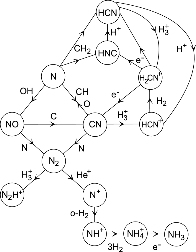
Because CN but not HCN (nor HNC) is destroyed by O, the abundance ratio CN:HCN increases as the C:O ratio increases. The chemical network is summarized in Fig. 6.

Figure 6: The principal reactions involved in the low–temperature chemistry of nitrogen–containing species, and specifically of CN, HCN and HNC.

5.2 Simplified analysis of the chemistry

We show now that an analysis of the principal reactions leading to the formation and destruction of CN and HCN leads to a simple analytical formula for the CN:HCN abundance ratio. When reactions (3) and (4) determine the abundance of CN,

$$n({\rm CN})=n({\rm CH})k_{\ref{equ3}}/k_{\ref{equ4}}=0.75n({\rm CH})$$

with the adopted values of the rate coefficients for these reactions at $T=10$ K.

We have seen already that HCN is formed in reaction (10), with a rate coefficient $k_{\ref{equ9}}=2.2\times{\rm 10^{-11}}$ $\rm cm^{3}\,s^{-1}$, and it is removed principally by H⁺ and H${}_{3}^{+}$, forming H₂CN⁺ (reactions 13 and 14). It follows that

$$k_{\ref{equ9}}n({\rm CH}_{2})n({\rm N})=k_{\rm L}n({\rm HCN})[n({\rm H}^{+})+n({\rm H}_{3}^{+})]f_{\rm CN},$$

where $k_{\rm L}$ is the Langevin rate coefficient which characterizes the reactions of HCN with H⁺ and H${}_{3}^{+}$.

Under the above assumptions, the CN:HCN ratio is proportional to the CH:${{\text{CH}_{\vphantom{\text{}}\text{2}}^{\vphantom{\text{}}\vphantom{\text{\smash[t]{2+}}}\text{}}}}$ ratio:

$$\frac{n({\rm CN})}{n({\rm HCN})}=\frac{k_{\ref{equ3}}}{k_{\ref{equ4}}}\frac{n({\rm CH})}{n({\rm CH}_{2})}f_{\rm CN}\frac{k_{\rm L}n({\rm e}^{-})}{k_{\ref{equ9}}n({\rm N})}\approx 100\frac{n({\rm CH})}{n({\rm CH}_{2})}\frac{n({\rm e}^{-})}{n({\rm N})}$$

where we have assumed that $n({\rm e}^{-})=n({{{{\mathrm{\mathrm{H}}_{\vphantom{\mathrm{}}\mathrm{}}^{\vphantom{\mathrm{}}\vphantom{\mathrm{\smash[t]{2+}}}\mathrm{+}}}}}})+n({{{{\mathrm{\mathrm{H}}_{\vphantom{\mathrm{}}\mathrm{3}}^{\vphantom{\mathrm{}}\vphantom{\mathrm{\smash[t]{2+}}}\mathrm{+}}}}}})$.

CH has its chemical origin in the reaction of He⁺ with CO

$${{{{\mathrm{\mathrm{He}}_{\vphantom{\mathrm{}}\mathrm{}}^{\vphantom{\mathrm{}}\vphantom{\mathrm{\smash[t]{2+}}}\mathrm{+}}}}+{}{{\mathrm{\mathrm{CO}}}}{{}\xrightarrow[]{\hskip 10.00002pt}{}}{{\mathrm{\mathrm{C}}_{\vphantom{\mathrm{}}\mathrm{}}^{\vphantom{\mathrm{}}\vphantom{\mathrm{\smash[t]{2+}}}\mathrm{+}}}}+{}{{\mathrm{\mathrm{O}}}}+{}{{\mathrm{\mathrm{He}}}}}}$$ (16)

for which the adopted value of the rate coefficient is $k_{\ref{equ13a}}=1.5\times{\rm 10^{-9}}$ $\rm cm^{3}\,s^{-1}$ (essentially Langevin). As CO depletes on to grains, there is competition with reaction (16) from the reactions of He⁺ with H₂,

$${{{{\mathrm{\mathrm{He}}_{\vphantom{\mathrm{}}\mathrm{}}^{\vphantom{\mathrm{}}\vphantom{\mathrm{\smash[t]{2+}}}\mathrm{+}}}}+{}{{\mathrm{\mathrm{H}}_{\vphantom{\mathrm{}}\mathrm{2}}^{\vphantom{\mathrm{}}\vphantom{\mathrm{\smash[t]{2+}}}\mathrm{}}}}{{}\xrightarrow[]{\hskip 10.00002pt}{}}{{\mathrm{\mathrm{H}}_{\vphantom{\mathrm{}}\mathrm{}}^{\vphantom{\mathrm{}}\vphantom{\mathrm{\smash[t]{2+}}}\mathrm{+}}}}+{}{{\mathrm{\mathrm{H}}}}+{}{{\mathrm{\mathrm{He}}}}}}$$ (17)

$${{{{\mathrm{\mathrm{He}}_{\vphantom{\mathrm{}}\mathrm{}}^{\vphantom{\mathrm{}}\vphantom{\mathrm{\smash[t]{2+}}}\mathrm{+}}}}+{}{{\mathrm{\mathrm{H}}_{\vphantom{\mathrm{}}\mathrm{2}}^{\vphantom{\mathrm{}}\vphantom{\mathrm{\smash[t]{2+}}}\mathrm{}}}}{{}\xrightarrow[]{\hskip 10.00002pt}{}}{{\mathrm{\mathrm{H}}_{\vphantom{\mathrm{}}\mathrm{2}}^{\vphantom{\mathrm{}}\vphantom{\mathrm{\smash[t]{2+}}}\mathrm{+}}}}+{}{{\mathrm{\mathrm{He}}}}}}$$

$k_{\ref{equ13b}}=4.0{\times 10^{-14}}$ $\rm cm^{3}\,s^{-1}$ (Schauer et al. 1989). Thus, the rate of production of carbon ions is $\zeta_{\rm He}n(\rm{He})f_{\rm C}$, where $\zeta_{\rm He}=0.5\zeta_{{\rm H}_{2}}$ is the rate of cosmic ray ionization of He and $f_{\rm C}=k_{\ref{equ13a}}n({\rm CO})/[k_{\ref{equ13b}}n({\rm H}_{2})+k_{\ref{equ13a}}n({\rm CO})].$

Most of the C⁺ ions produced in reaction (16) combine radiatively with H₂ to form CH${}_{2}^{+}$, which reacts rapidly with H₂, forming CH${}_{3}^{+}$ which then recombines dissociatively with electrons, yielding CH

$${{{{\mathrm{\mathrm{CH}}_{\vphantom{\mathrm{}}\mathrm{3}}^{\vphantom{\mathrm{}}\vphantom{\mathrm{\smash[t]{2+}}}\mathrm{+}}}}+{}{{\mathrm{\mathrm{e}}_{\vphantom{\mathrm{}}\mathrm{}}^{\vphantom{\mathrm{}}\vphantom{\mathrm{\smash[t]{2+}}}\mathrm{\mathrm{-}}}}}{{}\xrightarrow[]{\hskip 10.00002pt}{}}{{\mathrm{\mathrm{CH}}}}+{}{{\mathrm{\mathrm{H}}_{\vphantom{\mathrm{}}\mathrm{2}}^{\vphantom{\mathrm{}}\vphantom{\mathrm{\smash[t]{2+}}}\mathrm{}}}}}}$$ (18)

$${{{{\mathrm{\mathrm{CH}}_{\vphantom{\mathrm{}}\mathrm{3}}^{\vphantom{\mathrm{}}\vphantom{\mathrm{\smash[t]{2+}}}\mathrm{+}}}}+{}{{\mathrm{\mathrm{e}}_{\vphantom{\mathrm{}}\mathrm{}}^{\vphantom{\mathrm{}}\vphantom{\mathrm{\smash[t]{2+}}}\mathrm{\mathrm{-}}}}}{{}\xrightarrow[]{\hskip 10.00002pt}{}}{{\mathrm{\mathrm{CH}}}}+{}{{\mathrm{\mathrm{H}}}}+{\mathrm{\mathrm{H}}}}}$$ (19)

but also C and CH₂. The ratio $f_{\rm CH}=0.3$ is the fraction of the dissociative recombinations of CH${}_{3}^{+}$ which form CH and is significant for the CN:HCN abundance ratio. CH and ${{\text{CH}_{\vphantom{\text{}}\text{2}}^{\vphantom{\text{}}\vphantom{\text{\smash[t]{2+}}}\text{}}}}$ are destroyed by atomic O:

$${{{{\mathrm{\mathrm{CH}}}}+{}{{\mathrm{\mathrm{O}}}}{{}\xrightarrow[]{\hskip 10.00002pt}{}}{{\mathrm{\mathrm{CO}}}}{{\mathrm{\mathrm{H}}}}}}$$ (20)

$${{{{\mathrm{\mathrm{CH}}_{\vphantom{\mathrm{}}\mathrm{2}}^{\vphantom{\mathrm{}}\vphantom{\mathrm{\smash[t]{2+}}}\mathrm{}}}}+{}{{\mathrm{\mathrm{O}}}}{{}\xrightarrow[]{\hskip 10.00002pt}{}}{{\mathrm{\mathrm{CO}}}}+{}{{\mathrm{\mathrm{H}}}}+{}{{\mathrm{\mathrm{H}}}}}}$$ (21)

and

$${{{{\mathrm{\mathrm{CH}}_{\vphantom{\mathrm{}}\mathrm{2}}^{\vphantom{\mathrm{}}\vphantom{\mathrm{\smash[t]{2+}}}\mathrm{}}}}+{}{{\mathrm{\mathrm{O}}}}{{}\xrightarrow[]{\hskip 10.00002pt}{}}{{\mathrm{\mathrm{CO}}}}+{}{{\mathrm{\mathrm{H}}_{\vphantom{\mathrm{}}\mathrm{2}}^{\vphantom{\mathrm{}}\vphantom{\mathrm{\smash[t]{2+}}}\mathrm{}}}}}}$$ (22)

forming CO, and hence the elemental C:O ratio is, once again, a pertinent parameter for the CN:HCN ratio. So too are the rate coefficients for reactions (20), (21) and (22). We adopted the (temperature–independent) values of these rate coefficients in the NIST chemical kinetics database. All three reactions are rapid, with rate coefficients of the order of ${\rm 10^{-10}}$ $\rm cm^{3}\,s^{-1}$. The number density of CH is predicted to be $n({\rm CH})={\zeta_{\rm He}n({\rm He})f_{\rm C}f_{\rm CH}}/[{k_{\ref{equ3}}n({\rm N})+k_{\ref{equ14}}n({\rm O})}]$, Similarly that of CH₂ is predicted to be $n({\rm CH}_{2})={\zeta_{\rm He}n({\rm He})\,f_{\rm C}f_{\rm CH_{2}}/[k_{\ref{equ9}}n({\rm N})+(k_{\ref{equ15}}+k_{\ref{equ16}})n({\rm O})}]$. Assuming that $k_{\ref{equ15}}=k_{\ref{equ16}}$, one can deduce from the above equations that the CH:${{\text{CH}_{\vphantom{\text{}}\text{2}}^{\vphantom{\text{}}\vphantom{\text{\smash[t]{2+}}}\text{}}}}$ ratio is given by

$$\frac{n({\rm CH})}{n({\rm CH_{2}})}\,=\,\frac{f_{\rm CH}}{f_{\rm CH_{2}}}\,\frac{2k_{\ref{equ15}}n({\rm O})+k_{\ref{equ9}}n({\rm N})}{k_{\ref{equ14}}n({\rm O})+k_{\ref{equ3}}n({\rm N})}$$

It follows that $n({\rm CH})/n({\rm CH_{2}})$ depends on the ratio of the atomic N and O abundances and varies between extreme values of approximately 2, when $n({\rm O})\gg n({\rm N})$, and 0.2, when $n({\rm N})\gg n({\rm O})$. Model calculations (see Section 6.2) confirmed that the above approximation reproduces the calculated CN:HCN abundance ratio to within a factor of approximately 2 over most of the density range ${\rm 10^{4}}<n_{{\rm H}}<{\rm 10^{6}}$ ${\rm cm^{-3}}$. In the following Section 5.3, we consider the issue of the atomic nitrogen abundance in prestellar cores in more detail.

5.3 The abundance of atomic nitrogen in cores

Atomic abundances in prestellar cores are notoriously difficult to determine. Although the atomic fine structure transitions are, in principle, observable, it is difficult, in practice, to distinguish a component corresponding to dense, cold molecular material from emission arising from low density, hotter layers along the line of sight. The emission from photon dominated regions (PDRs), for example, tends to be stronger than that from cores.

The analysis in Section 5.2 suggests that the CH:CH₂ ratio is dependent on the abundances of atomic oxygen and nitrogen. Combining the expressions for the CH:CH₂ and the CN:HCN ratios, there follows the inequality

$$x({{{{\mathrm{\mathrm{N}}}}}})=n({{{{\mathrm{\mathrm{N}}}}}})/n({{{{\mathrm{\mathrm{H}}_{\vphantom{\mathrm{}}\mathrm{2}}^{\vphantom{\mathrm{}}\vphantom{\mathrm{\smash[t]{2+}}}\mathrm{}}}}}})\leq 100\frac{n({\rm CH})}{n({\rm CH_{2}})}\frac{x({\rm e})}{R({\rm CN:HCN})},$$

where $x({\rm e})$ denotes $n({\rm e})/n({\rm H}_{2})$ and $R({\rm CN:HCN})$ is the measured value of the CN:HCN ratio. The inequality arises from neglecting the destruction of CN by oxygen in reaction (7). We adopt $n({\rm CH})/n({\rm CH}_{2})\approx 1$ and estimate $x({\rm e})$ from Fig. 5 of Walmsley et al. (2004) as $5\times 10^{-8}n_{5}^{-0.5}$, where $n_{5}$ is $n({\rm H_{2}})$ in units of $10^{5}$ ${\rm cm^{-3}}$. From Table 3, we infer a typical value of 2 for $R({\rm CN:HCN})$ and conclude that the fractional atomic N abundance

$$n({{{{\mathrm{\mathrm{N}}}}}})/n_{{\rm H}}\lesssim 1.25{\times 10^{-6}}.$$

This value is considerably less than the cosmic nitrogen abundance ($n({{{{\mathrm{\mathrm{N}}}}}})/n_{{\rm H}}=7.9{\times 10^{-5}}$; Anders & Grevesse 1989) and implies that there is only a small fraction of elemental nitrogen in gaseous atomic form. Although some approximations were made when deriving this value (such as $n({\rm CH})/n({\rm CH}_{2})\approx 1$), our more precise and complete chemical modelling has confirmed that this estimate is essentially correct as long as the total gaseous nitrogen abundance is $n({{{{\mathrm{\mathrm{N}}}}}})/n_{{\rm H}}\leq{\rm 10^{-5}}$ (see Fig. 7). It follows that most of the elemental nitrogen must be in the form of gaseous N₂ or N-bearing solid compounds (e.g. NH₃ or N₂ ices). Indeed, for $n({{{{\mathrm{\mathrm{N}}}}}})/n_{{\rm H}}\leq{\rm 10^{-5}}$, steady–state models suggest that most of the nitrogen is in ices (see Section 6 as well as the discussion of Maret et al. 2006).

An analogous inequality, in terms of the measured CN:HCN ratio, can be derived for the fractional abundance of atomic oxygen, $x({\rm O})$. However, it is a much weaker constraint than the limit on $x({\rm N})$. Other observables, such as NO, provide stronger constraints on the fractional abundance of atomic oxygen (see A07).

6 Models

6.1 Steady state

Figure 7: Steady–state fractional abundances of nitrogen–containing species for a density $n_{{\rm H}}=10^{4}$ ${\rm cm^{-3}}$, a kinetic temperature $T=10$ K, and a cosmic ray ionization rate of $\zeta=10^{-17}$ s^-1. Upper panel: C:O=0.97 is held constant and the gas–phase nitrogen fractional abundance $\rm[N]_{gas}=n({{{{\mathrm{\mathrm{N}}}}}})/n_{{\rm H}}$ is varied from ${\rm 10^{-6}}$ to 6.4${\times 10^{-5}}$. Lower panel: $\rm[N]_{gas}=10^{-5}$ is held constant and the gas–phase C:O ratio is varied by changing $\rm[O]_{gas}$.

The timescale for the nitrogen chemistry to reach steady state is known to be large, relative to the free–fall time in a prestellar core, owing to the slow conversion of N to N₂ (see, for example, Flower et al. 2006). Our model calculations show that, with a cosmic ray ionization rate $\zeta=10^{-17}$ s^-1, this timescale is of the order of $10^{6}$ yr. As a consequence, the results of the time–dependent models of gravitational collapse depend on the initial composition which is adopted and the rate of dynamical evolution.

Following the discussion in Section 5, it is nevertheless instructive to examine the results of steady–state calculations (that is to say time independent and only in the gas phase), as functions of the fractions of elemental oxygen and nitrogen in the gas phase. In this way, an impression may be obtained of the dependence of the observables on the degrees of depletion, without the complications of the time dependence, which is considered in Section 6.2.

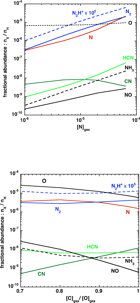
In the upper panel of Fig. 7, we present the fractional abundances of nitrogen–containing species in steady state for a density $n_{{\rm H}}=10^{4}$ ${\rm cm^{-3}}$, a kinetic temperature $T=10$ K, and a cosmic ray ionization rate of $\zeta=10^{-17}$ s^-1. For reaction (7), we adopted a temperature–independent rate coefficient ($4\times{\rm 10^{-11}}\,\rm cm^{3}\,s^{-1}$) although we note that there is some theoretical evidence that the rate of this reaction may decrease with temperature (Andersson & Markovi 2003). The fraction of elemental nitrogen in the gas phase varies from 0.017 to 1. We assume implicitly that the ‘missing’ nitrogen is in solid form. Following A07, we adopt a relative abundance of elemental carbon to oxygen in the gas phase $\rm C:O=0.97$. In the lower panel, the fractional abundance of elemental nitrogen in the gas phase is held constant at $n({{{{\mathrm{\mathrm{N}}}}}})/n_{{\rm H}}=10^{-5}$ and the C:O ratio is varied by changing the fractional abundance of oxygen in the gas phase $\rm[O]_{gas}$.

We see from Fig. 7 that, in steady state, there tends to be somewhat more molecular than atomic nitrogen in the gas phase. Species such as NH₃ and ${\rm N_{2}H^{+}}$ have abundances which are roughly proportional to N₂. The HCN abundance is relatively insensitive to changes in the gas phase C:O ratio but follows the gas-phase nitrogen abundance. On the other hand, CN and NO are sensitive to the C:O ratio. The net effect is that CN:HCN increases with C:O and decreases with the fraction of nitrogen in the gas phase.

Figure 8: The fractional abundances computed by the gravitational collapse model. We show in panel (a) results for the HCN abundance as a function of the CN:HCN ratio. In panel (b) we show the HCN abundance as a function of the ${{\text{N}_{\vphantom{\text{}}\text{2}}^{\vphantom{\text{}}\vphantom{\text{\smash[t]{2+}}}\text{}}\nolinebreak\text{H}_{\vphantom{\text{}}\text{}}^{\vphantom{\text{}}\vphantom{\text{\smash[t]{2+}}}\text{+}}}}$ abundance. In panel (c) the HCN abundance as a function of the NO abundance. The initial C:O ratio is assumed to be 0.97. Each point is labeled with the initial gas phase nitrogen abundance from ${\rm 10^{-6}}$ to 6.4${\times 10^{-5}}$. The initial steady state values (filled squares, green) are shown for comparison. Results for a density of $10^{5}$ ${\rm cm^{-3}}$ are given as blue open circles and for $10^{6}$ ${\rm cm^{-3}}$ as filled red circles. Data points are shown with black error bars. Data for ${{\text{N}_{\vphantom{\text{}}\text{2}}^{\vphantom{\text{}}\vphantom{\text{\smash[t]{2+}}}\text{}}\nolinebreak\text{H}_{\vphantom{\text{}}\text{}}^{\vphantom{\text{}}\vphantom{\text{\smash[t]{2+}}}\text{+}}}}$ towards Oph D and L 1517B are taken from Crapsi et al. (2005). In panel (d) we show the HCN:CO abundance ratio as a function of the CO fractional abundance, for different initial gas phase nitrogen abundances. For a given $\rm[N]_{gas}$, the ratios are followed during the collapse (snapshots at densities $10^{5}$, 4${\times 10^{5}}$ and $10^{6}$ ${\rm cm^{-3}}$ are shown) starting from the initial steady state. The CO abundance was taken from Caselli et al. (1999) for for L 1544, and for L 1517B both the HCN and CO abundances were taken from Tafalla et al. (2006).

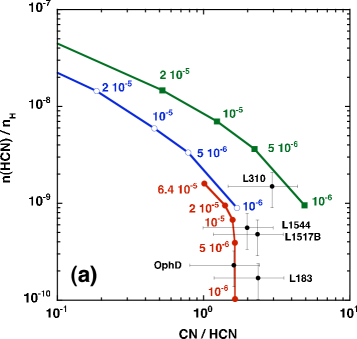
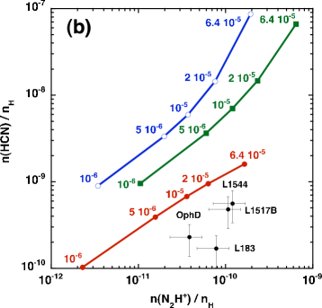
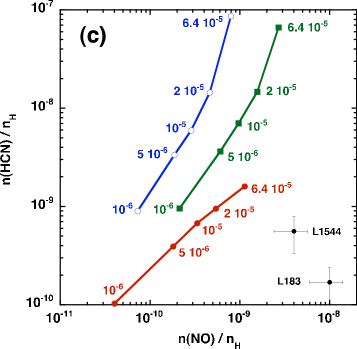
6.2 Gravitational collapse

A more satisfactory approach to comparing observational results with models is through a simulation of a gravitational collapse. In Fig. 8, we compare the observed values of the HCN abundance and the CN:HCN ratio with the predictions of models in which the density and the chemistry evolve following free–fall gravitational collapse. All neutral species are assumed to adsorb on to dust grains (of radius 0.5 $\mu{\rm m}$) with a sticking coefficient of unity and are desorbed by cosmic ray impacts (Flower et al. 2006). We assume that, initially, the chemical composition of the gas has attained steady state at a density $n_{{\rm H}}={\rm 10^{4}}$ ${\rm cm^{-3}}$. We make various assumptions concerning the amount of nitrogen initially in the gas phase (or, equivalently, the fraction which is initially in the form of nitrogen–containing ices on grain surfaces).

The fraction of elemental nitrogen in the ambient molecular medium which is in solid form is poorly known. There is evidence for ammonia ice in spectral profiles observed towards some young YSOs, with perhaps 15% of the abundance of water ice (Gibb et al. 2000), but no such evidence exists towards background stars; there is perhaps a substantial fraction of the nitrogen in the form of N₂ ice also. In prestellar cores, the abundance of ${\rm N_{2}H^{+}}$ places lower limits on the amount of gas–phase nitrogen, which we estimate conservatively to be about $10^{-6}$. Accordingly, we have varied the initial gas phase nitrogen abundance in our models in the range $10^{-6}\leq n({{{{\mathrm{\mathrm{N}}}}}})/n_{{\rm H}}\leq 6.4\times 10^{-5}$, where the upper limit corresponds to the value observed in diffuse interstellar gas (Sofia & Meyer 2001). Fig. 8 displays the fractional abundances computed in the course of the collapse, at densities $n_{{\rm H}}=10^{5}$ ${\rm cm^{-3}}$ and $n_{{\rm H}}=10^{6}$ ${\rm cm^{-3}}$. We show also, for comparison, the initial (steady state) values.

It may be seen from Fig. 8 that, at a density of $10^{5}$ ${\rm cm^{-3}}$  which is the more relevant value for the purpose of comparing with observations, reasonable agreement is obtained only for initial gas–phase nitrogen abundances close to $10^{-6}$ – in other words, close to the lower limit. Even so, the computed abundances do not fit well the observations of L 183 and Oph D; but we note that the density at the dust peak in L 183 approaches $10^{6}$ ${\rm cm^{-3}}$. Our model results are dependent also on the fraction of oxygen locked in ices, or, equivalently, on the initial gas–phase C:O ratio. It is possible that this ratio varies considerably from source to source, resulting in discrepancies when we compare observations with model predictions.

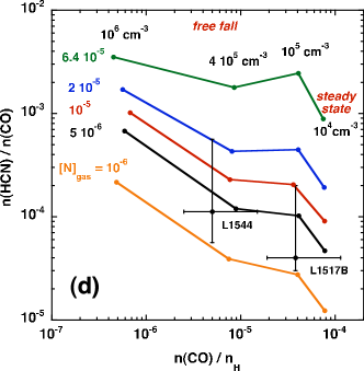
Figure 8 (bottom right panel) shows the HCN:CO abundance ratio as a function of the CO fractional abundance. For a given initial abundance of gaseous nitrogen $[\rm N]_{gas}$ ($=n({{{{\mathrm{\mathrm{N}}}}}})/n_{{\rm H}}$), the abundance ratio is followed along the collapse and values are shown at densities $n_{{\rm H}}=10^{5}$, 4${\times 10^{5}}$ and ${\rm 10^{6}}$ ${\rm cm^{-3}}$. The differential freeze-out of HCN and CO is evident. In all these models, CO depletes by two orders of magnitude. The behaviour of HCN regarding depletion is different in that it depends on the initial $\rm[N]_{gas}$. For a large initial $\rm[N]_{gas}=6.4{\times 10^{-5}}$, HCN depletes only a factor of 3 less than CO. However, at the other extreme value ($\rm[N]_{gas}={\rm 10^{-6}}$), HCN depletes 10 times less than CO. Observational values towards L 1544 (Caselli et al. 1999) and L 1517B (Tafalla et al. 2002) favour differential freeze-out between HCN and CO and thus low initial $\rm[N]_{gas}$.

We conclude from Fig. 8 that the models fail to explain the observations. One possible reason for this failure is our neglect of line-of-sight effects in the models used to construct Fig. 8. The observed quantities are column densities, which are integrals along the line of sight over a range of densities; our analysis neglects this effect. However, trial calculations for one source (L 1544; see Appendix D) suggest that including line-of-sight integration can reduce but not eliminate the discrepancies between model predictions and observations. Another possibility might be that the duration of the collapse is longer that the free-fall time. However, if this time is significantly increased, the abundance of gaseous CO drops too rapidly with increasing density (Flower et al. 2005). More important may be errors in the rate coefficients that we have used for some of the key reactions, discussed in Section 5. It is clear, for example, that our predictions relating to CN are sensitive to the rates of reactions (3), (4), and (10) at temperatures of the order of 10 K. Further progress in this field will require reliable determinations of the rate coefficients of these reactions at low temperatures.

We find that the values of the CN:HCN ratio observed in prestellar cores indicate that the fraction of nitrogen in the gas phase is likely to be considerably lower than the diffuse–gas value of $6.4\times 10^{-5}$. Nitrogen (like oxygen) may deplete on to grain surfaces at relatively low densities. Confirmation will require the identification of nitrogen–containing ices and estimates of their relative abundances. A rather similar conclusion has been reached by Maret et al. (2006) in a study of B68.

We finally note that our observations show HNC:HCN $\approx 2$, whereas the exhaustive theoretical study of Herbst et al. (2000) predicted HNC:HCN $\approx 1$. It is possible that enhanced line trapping in HNC, relative to HCN, results in our deriving an anomalously high HNC:HCN abundance ratio; but it is unlikely that this effect can explain fully the discrepancies with the model predictions. Maybe more relevant is the apparent correlation between the HNC:HCN ratio and freeze-out, as suggested by the results from Hirota et al. (1998) who show that the largest (resp. smallest) ratio is observed toward a strongly depleted core (resp. undepleted).

7 Concluding remarks

We have studied the behaviour of nitrogen–containing species, principally CN, HCN, and HNC, in the pre-protostellar cores L 183, L 1544, Oph D, L 1517B, and L 310. Our main conclusions are as follows.

• We observe that CN, HCN, and HNC remain present in the gas phase at densities above the typical density (3${\times 10^{4}}$ ${\rm cm^{-3}}$) at which CO depletes on to grains.

• The CN:HCN and HNC:HCN ratios are larger than unity in all objects and do not vary much within in each core. Whilst the differential freeze–out of CN and CO can be understood, the approximate constancy of the CN:HCN ratio cannot.

• The CN:HCN ratio puts upper limits on the abundance of atomic nitrogen in the gas phase, and the NO:HCN ratio constrains the C:O ratio. Though uncertain, the comparison between observations and models indicates that most of the nitrogen is locked into ices, even at densities probably as low as ${\rm 10^{4}}$ ${\rm cm^{-3}}$.

Our current knowledge of the chemistry of nitrogen–containing species is incompatible with the observed ratios. We recall that there exist large uncertainties in the rate coefficients, at low temperatures, for the key neutral–neutral reactions, discussed in Section 5, including those with atomic nitrogen. Essential to further progress in understanding the chemistry of nitrogen–containing species in pre-protostellar cores are measurements, at low temperatures, of at least some of these key reactions.

Appendix A Spectroscopic data

Table 4: Hyperfine structure in CN$(2-1)$ ($NJF\rightarrow N^{\prime}J^{\prime}F^{\prime}$); from Skatrud et al. (1983).

$N$  ,	$J$  ,	$F$ $\,\longrightarrow\,$	$N^{\prime}$  ,	$J^{\prime}$  ,	$F^{\prime}$	$\nu^{a}$	R.I.b
2  ,	3/2  ,	1/2 $\,\longrightarrow\,$	1  ,	1/2  ,	1/2	226663.685	0.0494
2  ,	3/2  ,	3/2 $\,\longrightarrow\,$	1  ,	1/2  ,	1/2	226679.341	0.0617
2  ,	3/2  ,	1/2 $\,\longrightarrow\,$	1  ,	1/2  ,	3/2	226616.520	0.0062
2  ,	3/2  ,	3/2 $\,\longrightarrow\,$	1  ,	1/2  ,	3/2	226632.176	0.0494
2  ,	3/2  ,	5/2 $\,\longrightarrow\,$	1  ,	1/2  ,	3/2	226659.543	0.1667
2  ,	3/2  ,	1/2 $\,\longrightarrow\,$	1  ,	3/2  ,	1/2	226287.393	0.0062
2  ,	3/2  ,	3/2 $\,\longrightarrow\,$	1  ,	3/2  ,	1/2	226303.049	0.0049
2  ,	5/2  ,	3/2 $\,\longrightarrow\,$	1  ,	3/2  ,	1/2	226875.896	0.1000
2  ,	3/2  ,	1/2 $\,\longrightarrow\,$	1  ,	3/2  ,	3/2	226298.896	0.0049
2  ,	3/2  ,	3/2 $\,\longrightarrow\,$	1  ,	3/2  ,	3/2	226314.552	0.0120
2  ,	3/2  ,	5/2 $\,\longrightarrow\,$	1  ,	3/2  ,	3/2	226341.919	0.0053
2  ,	5/2  ,	3/2 $\,\longrightarrow\,$	1  ,	3/2  ,	3/2	226887.399	0.0320
2  ,	5/2  ,	5/2 $\,\longrightarrow\,$	1  ,	3/2  ,	3/2	226874.183	0.1680
2  ,	3/2  ,	3/2 $\,\longrightarrow\,$	1  ,	3/2  ,	5/2	226332.519	0.0053
2  ,	3/2  ,	5/2 $\,\longrightarrow\,$	1  ,	3/2  ,	5/2	226359.887	0.0280
2  ,	5/2  ,	3/2 $\,\longrightarrow\,$	1  ,	3/2  ,	5/2	226905.366	0.0013
2  ,	5/2  ,	5/2 $\,\longrightarrow\,$	1  ,	3/2  ,	5/2	226892.151	0.0320
2  ,	5/2  ,	7/2 $\,\longrightarrow\,$	1  ,	3/2  ,	5/2	226874.764	0.2667

• $a$: Rest frequency in MHz.

• $b$: Relative intensities, with their sum normalized to unity.
  

Appendix B Data reduction

Data reduction was done with the CLASS90 software from the GILDAS program suite. We summarize here the reduction of the frequency–switched spectra obtained with the VESPA autocorrelator facility at the IRAM 30 m radio telescope.

All spectra were corrected first from the instrumental spectral transfer function. The resulting spectra were then folded and averaged (each folded spectrum being weighted by the effective rms of the residuals after baseline subtraction). A zero–order polynomial was fitted to the resulting spectrum to compute the final rms. Whenever platforming was present in the data, the spectrum was split into as many parts as needed, and each part was treated individually with a first–order polynomial in order to adjust the continuum level. The concatenated sub-parts were then treated as a single spectrum. This method proved to be robust. In some cases, the amplitude of ripples was large enough to require special treatment. Ripples were subtracted by fitting a sine wave to the spectrum, using an improved version of sine fitting, as compared with the default CLASS90 procedure. In the case of a spectrum presenting ripples, channels in the spectral windows (where there is presumably some line emission) were replaced by a sine wave, determined by the first–guess parameters (amplitude, period and phase). As the critical parameter in the sine wave minimization proved to be the period, the minimization was repeated for several values of the period. In all cases, this algorithm converged to an acceptable solution, as indicated by the residuals and inspection by eye.

Appendix C Column density derivation

Table 5: Conversion factor, $N_{0}$ (in ${\rm 10^{12}}$${\rm cm^{-2}}$/(${\rm K\,km\,s^{-1}}$)), at an excitation temperature $T_{{\rm ex}}=8$ K (see Eq. 24).

Molecule	Transition	$\nu^{a}$	$\delta v^{b}$	$B_{{\rm{eff}}}^{c}$	$B$	$\mu_{0}$	R.I.d	$Q^{e}$	$N_{0}/\rm R.I.$
		MHz	${\rm km\,s^{-1}}$		MHz	debye
CN	$(1-0)$	113520.414	0.052	0.74	56693.470	1.45	0.0184	3.3	293
CN	$(2-1)$	226882.000	0.053	0.50
HCN	$(1-0)$	88633.936	0.066	0.77	44315.976	2.9852	0.1111	4.1	16.4
${\rm{}^{13}CN}$	$(1-0)$	108780.201	0.063	0.77	54353.130	1.45	0.194	3.4	29.5
H${\rm{}^{13}CN}$	$(1-0)$	86342.251	0.054	0.75	43170.127	2.9852	0.5556	4.2	3.4
HN${\rm{}^{13}C}$	$(1-0)$	87090.850	0.068	0.78	45331.980	3.05	1.000	4.0	1.7
HC${\rm{}^{15}N}$	$(1-0)$	86054.9664	0.067	0.78	43027.648	2.9852	1.000	4.2	1.9
${\rm N_{2}H^{+}}$	$(1-0)$	93171.621	0.068	0.78	46586.880	3.40	0.037	3.9	35.2

• ^a Frequency of the HFS component considered for which we compute the flux $W$.

• ^b Spectral resolution in ${\rm km\,s^{-1}}$.

• ^c Beam efficiency. The forward efficiency at 3 mm is $F_{{\rm{eff}}}=0.95$, and 0.91 at 1.3 mm.

• ^d Relative intensity of the HFS component. The total flux in Eq. 24 is $W_{\rm tot}=W/$R.I.

• ^e Partition function computed as $Q=\displaystyle\sum_{J=0}^{20}(2J+1)\exp^{-\frac{hBJ(J+1)}{k_{\rm B}T_{{\rm ex}}}}$, where $B$ is the rotational constant.

All column densities are derived assuming optically thin emission with levels populated in LTE at the excitation temperature $T_{{\rm ex}}$. Under these assumptions, the column density is directly proportional to the integrated flux in the line $W_{\rm tot}$. From a transition $J_{\rm u}\rightarrow J_{\rm l}$ between energy levels $E_{\rm u}$ and $E_{\rm l}$ (corresponding to an energy $T_{0}=(E_{\rm u}-E_{\rm l})/k_{\rm B}$), one can compute the total column density of the molecule as

$$N_{\rm tot}=\frac{3\epsilon_{0}h}{2\pi^{2}}\,\frac{1}{J_{\rm u}\mu_{0}^{2}}\,\frac{Q\,{\rm e}^{E_{\rm l}/k_{\rm B}T_{{\rm ex}}}\,W_{\rm tot}}{\Delta J_{\nu}[1-\exp(-\frac{T_{0}}{T_{{\rm ex}}})]}$$ (23)

in SI units, where $\Delta J_{\nu}=J_{\nu}(T_{{\rm ex}})-J_{\nu}(T_{{\rm bg}})$, with $J_{\nu}(T)=T_{0}/[\exp(T_{0}/T)-1]$, and $\mu_{0}$ is the dipole moment; $\epsilon_{0}$ is the permittivity of free space. Numerically, we obtain

$$N_{\rm tot}=\frac{8{\times 10^{12}}}{J_{\rm u}\mu_{D}^{2}}\,\frac{Q\,e^{E_{\rm l}/k_{\rm B}T_{{\rm ex}}}\,W_{\rm tot}}{\Delta J_{\nu}[1-\exp(-\frac{T_{0}}{T_{{\rm ex}}})]}=N_{0}(T_{{\rm ex}})\,W_{\rm tot}$$ (24)

with $W_{\rm tot}$ in ${\rm K\,km\,s^{-1}}$and $N_{\rm tot}$ in cm^-2; $\mu_{D}$ is the dipole moment in debye. We have introduced the conversion factor, $N_{0}$, which depends on the molecular properties and the excitation temperature. It is to be noted that, in the case of resolved hyperfine structure, $W_{\rm tot}$ is the total integrated intensity of the hyperfine multiplet, i.e. of the rotational transition. Values of $N_{0}$ are given in Table 5 for the observed molecules and at an excitation temperature $T_{{\rm ex}}=8$ K (see HWFP08).

Figure 9: Ratio of the total integrated intensities $W_{\rm tot}$ of the molecules indicated in each panel, as a function of the offset from the dust emission peak. For each molecule, $W_{\rm tot}$ is derived from the values in the corresponding Table divided by the relative intensity of the HFS component, when resolved. Filled and open circles distinguish between the two cut directions. Open triangles are 5$\sigma$ upper limits. From top to bottom, L 183, L 1544, Oph D, L 1517B, and L 310.

Appendix D Modelling of the prestellar core L 1544

In order to interpret our observations of L 1544, we make use of the model of one–dimensional, free–fall gravitational collapse used in our previous study (A07). This model incorporates dust grain coagulation and a time–dependent chemistry, including the reactions listed in Section 5 above, which are directly relevant to the present work. We assume a constant kinetic temperature, $T=10$ K, and a cosmic ray ionization rate, $\zeta=10^{-17}$ s^-1. Further information on the model may be found in Flower et al. (2005).

An important aspect of the interpretation is to connect, as realistically as possible, the abundance profiles (i.e. the number density of species X, $n$(X) as a function of the total density, $n_{{\rm H}}=2n({\rm H}_{2})+n({\rm H})$), which are the output of the model, to the observed variations in L 1544 of column densities, $N$(X), with impact parameter $r$. In order to make this connection, we proceed as follows:

• we relate the gas density at $r$ to the central density by means of the relation

  $$n_{{\rm H}}(r)=n_{{\rm H}}(0)/[1+(r/r_{2})^{\alpha}]$$

  Tafalla et al. (2002), where $r$ is the offset from centre, $r=0$, and $r_{2}$ is the radial distance over which the density decreases to $n_{{\rm H}}(0)/2$. Following Tafalla et al. (2002), we adopt $r_{2}=20$^′′(equivalent to 0.014 pc at the distance of L 1544) and $\alpha=2.5$; the central density $n(0)={\rm 10^{6}}$ ${\rm cm^{-3}}$ (A07), which is somewhat smaller than the value reported in Table LABEL:tab:cores for this object but within the probable uncertainties of its determination.

• Using the computed values of $n$(X) vs $n_{{\rm H}}$, we calculate the corresponding column density, $N$(X), by integrating along the line of sight for any given value of $r$ in the adopted range $0\leq r\leq 120$ arcsec, over which the density $n_{{\rm H}}(r)$ decreases from ${\rm 10^{6}}$ ${\rm cm^{-3}}$ to $1.1{\times 10^{4}}$ ${\rm cm^{-3}}$.

• Finally, the column densities are convolved with a Gaussian profile with a (1/e) radius of 15^′′, corresponding to a HPBW of 25^′′, in order to simulate approximately the IRAM 30 m telescope beam at 100 GHz.

As will be seen below, the consequence of this procedure is a significant damping of the variations in the computed abundance profiles, owing partly to the effect of integrating along the line of sight and hence over a range of densities, and partly to the Gaussian beam averaging.

We consider first the predictions of the chemical model, and specifically the abundances of nitrogen–containing species. We turn our attention then to the Gaussian–beam averaged column densities, and their comparison with the observations.

D.1 Abundance profiles

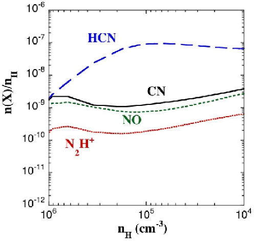
In Fig. 10 are plotted the fractional abundance profiles of CN, HCN, NO and N₂H⁺; note that the $x$-axis has been reversed in order to facilitate the comparison with later Figures, in which the $x$-coordinate is the offset from the centre, where the density of the medium is highest. We see from Fig. 10 that, at low densities, the fractional abundance of HCN exceeds that of CN, by a factor which approaches two orders of magnitude when $n_{{\rm H}}\approx{\rm 10^{5}}$ ${\rm cm^{-3}}$. The fractional abundance of HCN decreases towards the maximum density of ${\rm 10^{6}}$ ${\rm cm^{-3}}$, where $n({\rm HCN})\approx n({\rm CN})$. This behaviour can be understood by reference to the discussion in Section 5 above: CN is formed and destroyed in reactions (3, 4) which involve atomic nitrogen; HCN, on the other hand, is formed in reaction (10) with N but destroyed in reactions with H⁺ and H${}_{3}^{+}$ that ultimately lead to CN. Consequently, as the density of the medium increases, and neutral species begin to freeze on to the grains, the fractional abundance of HCN falls, whereas the fractional abundance of CN remains roughly constant until, finally, CN too freezes on to the grains.

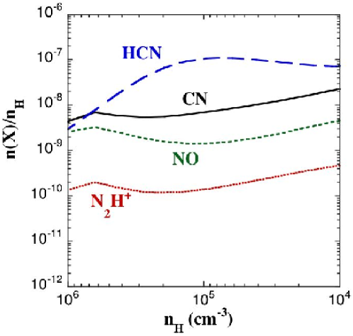
We have already seen in Section 2 that the ratio of the column densities of HCN and CN, which is of the order of 1 in L 1544, shows little variation across this and the other sources in our sample. Thus, it seems unlikely that the fractional abundance profiles of HCN and CN seen in the upper panel of Fig. 10 are compatible with the observed column densities, given that the ratio $n({\rm HCN})/n({\rm CN})$ varies by approximately 2 orders of magnitude over the range of density ${\rm 10^{4}}\leq n_{{\rm H}}\leq{\rm 10^{6}}$ cm^-3; this tentative conclusion is confirmed by the analysis in the following Section D.2. It appears that the observations are indicating that the natures of both the formation and the destruction processes are similar for both these species. This realization led us to consider the possibility that reaction (4), which destroys CN, may have a small barrier, significant at the low temperatures relevant here ($T\lesssim 10$ K) but difficult to detect by measurements at higher temperatures. A similar situation may obtain for the analogous reaction (2) of NO with N. Accordingly, we show, in the lower panel of Fig. 10 the results which are obtained on introducing a barrier of 25 K to both reaction (2) and reaction (4); we note that the adopted barrier size is arbitrary, the only requirement being that it should be small.

Small barriers can arise when the potential energy curves involved in the atom–molecule reaction exhibit (much larger) barriers for certain angles of approach but no barrier for others. In order to determine the thermal rate coefficient, the probability of the reaction must be averaged over the relative collision angle. If the rate coefficient is then fitted to an Arrhenius form,

$$k(T)=\gamma(T/300)^{\alpha}\exp(-\beta/T),$$

small, positive values of $\beta$ may be interpreted as the angle–averaged value of the reaction barrier; see Andersson & Markovi (2003).

It is clear from Fig. 10 that the small reaction barrier has the effect of enhancing the fractional abundance of CN and reducing the amplitude of the variation in the ratio $n({\rm HCN})/n({\rm CN})$. We shall see in the following Section D.2 that this variation is damped further when the ratio of the corresponding Gaussian–beam averaged column densities is considered.

Figure 10: The number densities of CN, HCN, NO and N₂H⁺, relative to $n_{{\rm H}}=2n({\rm H}_{2})+n({\rm H})$, as predicted by a model of gravitational free–fall collapse. The lower panel illustrates the effects of introducing a barrier of 25 K to both reaction (2) and reaction (4).

Figure 11: The column densities of CN, HCN, NO and N₂H⁺, relative to H₂, as predicted by the model described in Section D. The lower panel illustrates the effects of introducing a barrier of 25 K to both reaction (2) and reaction (4).

The results in Fig. 10 have been obtained assuming that the grain–sticking probability was unity for all species, and that the elemental abundance ratio $\rm C:O=0.97$, i.e. a marginally oxygen–rich medium. This value of the C:O ratio was an outcome of the modelling by A07 of observations of NO and ${{\text{N}_{\vphantom{\text{}}\text{2}}^{\vphantom{\text{}}\vphantom{\text{\smash[t]{2+}}}\text{}}\nolinebreak\text{H}_{\vphantom{\text{}}\text{}}^{\vphantom{\text{}}\vphantom{\text{\smash[t]{2+}}}\text{+}}}}$ in L 1544. These authors investigated also the consequences of varying the values of the sticking coefficient for atomic C, N and O, and the initial value of the N:N₂ abundance ratio. We recall that increasing the elemental C:O abundance ratio further has the consequence of reducing the HCN:CN ratio, thereby improving the agreement with the observations. On the other hand, the CN:NO ratio also rises, and the values of this ratio in Fig. 10, where $n({\rm CN})>n({\rm NO})$, already exceed the values of the corresponding column density ratio, observed in L 1544, where $N({\rm CN})<N({\rm NO})$ by typically an order of magnitude. It is possible that selective variations in the values of the sticking probability, or in the initial N:N₂ abundance ratio, might alleviate some of these discrepancies. However, whilst there remain such large uncertainties in the values of the rate coefficients for the key neutral–neutral reactions, discussed in Section 5, it would perhaps be premature to investigate further the consequences of modifying the values of other (and equally uncertain) parameters, in an attempt to improve the agreement between the models and the observations. Our aim here is to point to the discrepancies and highlight the uncertainties; and it seems unlikely that further progress can be made until the rates of at least some of the key reactions have been measured at low temperatures.

D.2 Column densities

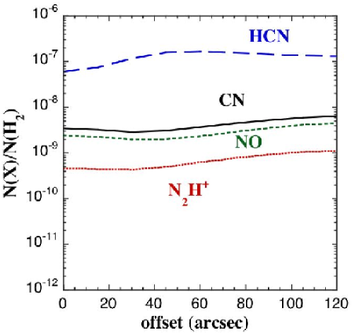
In Fig. 11 are shown the computed column densities of CN, HCN, NO and ${\rm N_{2}H^{+}}$, relative to the column density of ${\rm H_{2}}$. The fractional abundances of these species, relative to $n_{{\rm H}}$, derive from the models discussed in the previous Section D.1.

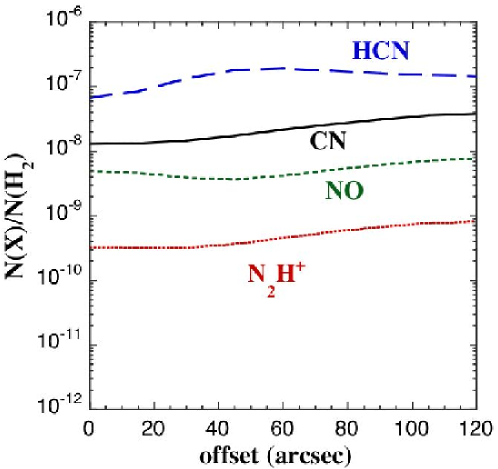
At zero offset, the line of sight passes through regions with densities covering the entire range of the model, $1.0{\times 10^{6}}{\rm cm^{-3}}\geq n_{{\rm H}}\geq 1.1{\times 10^{4}}$ ${\rm cm^{-3}}$. Consequently, the column density ratio, $N({\rm HCN})/N({\rm H}_{2})\gg n({\rm HCN})/n_{{\rm H}}$, evaluated at the peak density $n_{{\rm H}}={\rm 10^{6}}$ ${\rm cm^{-3}}$; further smoothing is introduced by the Gaussian–beam averaging. The overall effect of the line–of–sight and Gaussian–beam averaging is a flattening of the column density profiles (Fig. 11), compared with the fractional abundance profiles (Fig. 10). Comparing the two panels of Fig. 11, we see that the introduction of the small barriers to the reactions of CN and NO with N reduces substantially the $N({\rm HCN})/N({\rm CN})$ column density ratio. Although they do not attain the observed value, of the order of $1$, the computed values of $N({\rm HCN})/N({\rm CN})$ in the lower panel of Fig. 11 are clearly more compatible with the observations of L 1544 than are those in the upper panel.

Table 6: Line properties (main beam temperature scale) and total column densities derived towards L 183. Numbers in parentheses are powers of 10.

Line	$\delta x$	$\delta y$	$T_{\rm mb}$	$W$	$\Delta v$e	$N_{\rm tot}$f	$N({\rm H_{2}})$	$N_{\rm tot}/2N({\rm H_{2}})$g
	′′	′′	mK	m${\rm K\,km\,s^{-1}}$	${\rm km\,s^{-1}}$	${\rm 10^{12}}$ ${\rm cm^{-2}}$	${\rm 10^{22}}$ ${\rm cm^{-2}}$
CN	0	0	700$\pm$ 60	180$\pm$ 10	0.26	53	7.0	3.8$(-$10)
	-40	0	600$\pm$ 70	140$\pm$ 12	0.23	41	3.3	6.2$(-$10)
	-20	0	650$\pm$ 70	135$\pm$ 10	0.21	40	6.1	3.3$(-$10)
	20	0	590$\pm$ 80	110$\pm$ 10	0.19	34	4.8	3.5$(-$10)
	40	0	455$\pm$ 80	60$\pm$ 10	0.13	18$\pm$2.9	2.8	3.2$(-$10)
	0	-40	580$\pm$ 85	130$\pm$ 10	0.22	38	3.9	4.9$(-$10)
	0	-20	755$\pm$ 60	160$\pm$ 7	0.21	47	5.6	4.2$(-$10)
	0	20	670$\pm$ 90	140$\pm$ 10	0.21	41	6.3	3.3$(-$10)
	0	40	660$\pm$ 80	175$\pm$ 15	0.26	48	5.7	4.2$(-$10)
${\rm{}^{13}CN}$a	0	0	115$\pm$ 12	28$\pm$ 2	0.24	0.82	7.0	5.9$(-$12)
	-40	0	75$\pm$ 25	$<$ 18		$<$ 0.53	3.3	$<$8.0$(-$12)
	-20	0	100$\pm$ 20	21$\pm$ 3	0.21	0.62 $\pm$ 0.09	6.1	5.1$(-$12)
	20	0	65$\pm$ 20	15$\pm$ 3	0.23	0.44 $\pm$ 0.09	4.8	4.6$(-$12)
	40	0	100$\pm$ 20	$<$ 18		$<$ 0.53	2.8	9.5$(-$12)
	0	-40	65$\pm$ 20	15$\pm$ 3	0.23	0.44 $\pm$ 0.09	3.9	5.6$(-$12)
	0	-20	95$\pm$ 20	16$\pm$ 3	0.17	0.47 $\pm$ 0.09	5.6	4.2$(-$12)
	0	20	115$\pm$ 20	30$\pm$ 2	0.26	0.88	6.3	7.0$(-$12)
	0	40	115$\pm$ 20	32$\pm$ 4	0.28	0.94 $\pm$ 0.12	5.7	8.2$(-$12)
H${\rm{}^{13}CN}$b	0	0	200$\pm$ 11	98$\pm$ 4	0.49	0.34	7.0	2.4$(-$12)
	-40	0	135$\pm$ 17	46$\pm$ 5	0.34	0.16 $\pm$ 0.02	3.3	2.4$(-$12)
	-20	0	250$\pm$ 20	123$\pm$ 7	0.49	0.42	6.1	3.4$(-$12)
	20	0	195$\pm$ 15	94$\pm$ 4	0.48	0.32	4.8	3.3$(-$12)
	40	0	160$\pm$ 15	80$\pm$ 5	0.50	0.27	2.8	4.8$(-$12)
	0	-40	180$\pm$ 35	76$\pm$ 7	0.42	0.26	3.9	3.3$(-$12)
	0	-20	245$\pm$ 18	91$\pm$ 5	0.37	0.31	5.6	2.8$(-$12)
	0	20	230$\pm$ 17	100$\pm$ 4	0.43	0.34	6.3	2.7$(-$12)
	0	40	230$\pm$ 18	101$\pm$ 5	0.44	0.34	5.7	3.0$(-$12)
HN${\rm{}^{13}C}$c	0	0	935$\pm$ 20	540$\pm$ 4	0.58	0.93	7.0	6.6$(-$12)
	-40	0	788$\pm$ 35	475$\pm$ 7	0.60	0.82	3.3	1.2$(-$11)
	-20	0	930$\pm$ 35	570$\pm$ 7	0.61	0.99	6.1	8.1$(-$12)
	20	0	710$\pm$ 33	433$\pm$ 7	0.61	0.75	4.8	7.8$(-$12)
	40	0	440$\pm$ 35	275$\pm$ 13	0.62	0.48	2.8	8.6$(-$12)
	0	-40	840$\pm$ 35	445$\pm$ 6	0.53	0.77	3.9	9.9$(-$12)
	0	-20	955$\pm$ 30	517$\pm$ 6	0.54	0.89	5.6	7.9$(-$12)
	0	20	1030$\pm$ 35	700$\pm$ 7	0.58	1.2	6.3	9.5$(-$12)
	0	40	1115$\pm$ 30	712$\pm$ 7	0.64	1.2	5.7	1.1$(-$11)
${\rm N_{2}H^{+}}$d	0	0	1356$\pm$ 20	309$\pm$ 6	0.23	10.9	7.0	7.8$(-$11)
	80	0	264$\pm$ 26	67$\pm$ 5	0.25	0.786	1.5	2.6$(-$11)
	60	0	160$\pm$ 24	40$\pm$ 7	0.25	1.41$\pm$ 0.246	2.0	3.5$(-$11)
	40	0	564$\pm$ 37	153$\pm$ 11	0.27	5.39	2.8	9.6$(-$11)
	20	0	1037$\pm$ 30	239$\pm$ 9	0.23	8.41	4.8	8.8$(-$11)
	-20	0	1209$\pm$ 29	283$\pm$ 9	0.23	9.96	6.1	8.2$(-$11)
	-40	0	709$\pm$ 21	164$\pm$ 6	0.23	5.77	3.3	8.7$(-$11)
	-60	0	408$\pm$ 19	103$\pm$ 6	0.25	3.63	2.3	7.9$(-$11)
	-80	0	327$\pm$ 26	79$\pm$ 8	0.24	2.78$\pm$ 0.282	2.4	5.8$(-$11)

• Error bars are 1$\sigma$, and upper limits on $W$ and $N_{\rm tot}$ are at the 5$\sigma$ level. A final calibration uncertainty on the column density of 10% has been adopted, unless smaller than 1$\sigma$. We adopt a systematic uncertainty on the dust column density of 30% which reflects the uncertainties on $T_{\rm dust}$ and $\kappa_{\nu}$.

• ^a Strongest component at 108780.2010 MHz, with R.I. = 0.194.

• ^b Strongest component at 86340.1840 MHz, with R.I. = 0.556.

• ^c The integrated intensity includes the three blended HFS components.

• ^d Weakest HFS component at 93171.6210 MHz with R.I. = 0.037 unless specified. At offsets (80^′′,0^′′) we use the isolated HFS component at 93176.2650 MHz with R.I.=0.1111 (see Table 5).

• ^e $\Delta v=W/T_{\rm mb}$ is the equivalent width. Error bars are 1$\sigma$, and upper limits on $W$ and

• ^f $N_{\rm tot}=W\times N_{0}/R.I.$

• ^g Fractional abundances with respect to H assuming $N({\rm H})=2N({\rm H_{2}})$.

Table 7: As Table 6 but for lines observed towards L 1544.

Line	$\delta x$	$\delta y$	$T_{\rm mb}$	$W$	$\Delta v$	$N_{\rm tot}$	$N({\rm H_{2}})$	$N_{\rm tot}/2N({\rm H_{2}})$
	′′	′′	mK	m${\rm K\,km\,s^{-1}}$	${\rm km\,s^{-1}}$	${\rm 10^{12}}$ ${\rm cm^{-2}}$	${\rm 10^{22}}$ ${\rm cm^{-2}}$
CNa	0	0	1658$\pm$ 65	688$\pm$ 35	0.41	202	6.7	1.5$(-$9)
	-40	-40	325$\pm$ 63	$<$ 50		$<$15
	-20	-20	1171$\pm$ 103	422$\pm$ 27	0.36	124	2.8	2.2$(-$9)
	20	20	771$\pm$ 67	304$\pm$ 52	0.39	89.1$\pm$15.2	3.6	1.2$(-$9)
	40	40	729$\pm$ 94	254$\pm$ 20	0.35	74.4	1.2	3.2$(-$9)
	-40	40	1257$\pm$ 105	565$\pm$ 62	0.45	166$\pm$18	3.6	2.3$(-$9)
	-20	20	1641$\pm$ 66	745$\pm$ 106	0.45	218$\pm$31	4.9	2.2$(-$9)
	20	-20	1569$\pm$ 93	587$\pm$ 52	0.37	172	4.4	2.0$(-$9)
	40	-40	1124$\pm$ 80	296$\pm$ 30	0.26	86.7	1.6	2.8$(-$9)
${\rm{}^{13}CN}$	0	0	166$\pm$15	73$\pm$4	0.44	2.17	6.7	1.6$(-$11)
	-40	-40	$<$ 60	$<$ 20		$<$0.60
	-20	-20	108$\pm$19	37$\pm$4	0.34	1.10$\pm$0.13	2.8	2.0$(-$11)
	20	20	85$\pm$19	21$\pm$3	0.26	0.65$\pm$0.10	3.6	9.1$(-$12)
	40	40	55$\pm$20	20$\pm$5	0.35	0.58	1.2	2.5$(-$11)
	-60	60	79$\pm$19	11 $\pm$3	0.14	0.33	2.3	7.3$(-$12)
	-40	40	118$\pm$20	46$\pm$6	0.39	1.36$\pm$0.19	3.6	1.9$(-$11)
	-20	20	166$\pm$17	47$\pm$3	0.29	1.40	4.9	1.4$(-$11)
	20	-20	165$\pm$18	58$\pm$4	0.35	1.72	4.4	2.0$(-$11)
	40	-40	94$\pm$20	23$\pm$3	0.25	0.71$\pm$0.10	1.6	2.3$(-$11)
	60	-60	$<$ 60	$<$ 20		$<$0.60
H${\rm{}^{13}CN}$	0	0	746$\pm$ 12	315$\pm$ 5	0.42	1.1	6.7	8.2$(-$12)
	-60	-60	$<$ 55	$<$ 10		$<$0.03
	-40	-40	$<$ 57	$<$ 20		$<$0.07
	-20	-20	432$\pm$ 20	172$\pm$ 10	0.40	0.58	2.8	1.1$(-$11)
	20	20	405$\pm$ 18	163$\pm$ 10	0.40	0.55	3.6	7.7$(-$12)
	40	40	207$\pm$ 19	61$\pm$ 3	0.29	0.21	1.2	9.0$(-$12)
	60	60	117$\pm$ 23	41$\pm$ 6	0.35	0.14$\pm$0.02	$<0.75$
	-60	60	270$\pm$ 25	111$\pm$ 9	0.41	0.38	2.3	8.4$(-$12)
	-40	40	396$\pm$ 20	191$\pm$ 6	0.48	0.65	3.6	8.9$(-$12)
	-20	20	574$\pm$ 18	260$\pm$ 8	0.45	0.88	4.9	9.0$(-$12)
	20	-20	591$\pm$ 18	243$\pm$ 7	0.41	0.83	4.4	9.4$(-$12)
	40	-40	313$\pm$ 19	132$\pm$ 12	0.42	0.45	1.6	1.4$(-$11)
	60	-60	61$\pm$ 19	22$\pm$ 4	0.37	0.07$\pm$0.01
HN${\rm{}^{13}C}$	0	0	1758$\pm$ 29	1282$\pm$ 49	0.73	2.2	6.7	1.6$(-$11)
	-40	-40	$<$ 204	$<$ 80		$<$0.14
	-20	-20	945$\pm$ 67	661$\pm$ 58	0.70	1.1	2.8	2.0$(-$11)
	20	20	1066$\pm$ 67	710$\pm$ 90	0.67	1.2$\pm$0.15	3.6	1.7$(-$11)
	40	40	563$\pm$ 65	312$\pm$ 54	0.56	0.53$\pm$0.09	$<0.75$
	-40	40	914$\pm$ 67	716$\pm$ 58	0.78	1.2	3.6	1.6$(-$11)
	-20	20	1577$\pm$ 66	1223$\pm$ 77	0.78	2.1	4.9	2.1$(-$11)
	20	-20	1536$\pm$ 68	853$\pm$ 69	0.56	1.5	4.4	1.7$(-$11)
	40	-40	908$\pm$ 71	585$\pm$ 38	0.64	0.99	1.6	3.1$(-$11)
HC${\rm{}^{15}N}$	0	0	258$\pm$ 19	136$\pm$ 13	0.53	0.26	6.7	1.9$(-$12)
	-40	-40	$<$ 108	$<$ 60		$<$ 0.12
	-20	-20	142$\pm$ 35	58$\pm$ 7	0.41	0.11	2.8	2.0$(-$12)
	20	20	163$\pm$ 34	80$\pm$ 7	0.49	0.15	3.6	2.1$(-$12)
	40	40	130$\pm$ 38	$<$ 40		$<$ 0.08	1.2	3.4$(-$12)
	-40	40	217$\pm$ 36	92$\pm$ 10	0.42	0.17$\pm$0.02	3.6	2.3$(-$12)
	-20	20	235$\pm$ 36	110$\pm$ 22	0.46	0.21	4.9	2.1$(-$12)
	20	-20	246$\pm$ 34	110$\pm$ 10	0.44	0.21	4.4	2.4$(-$12)
	40	-40	246$\pm$ 38	100$\pm$ 10	0.41	0.19	1.6	6.0$(-$12)
${\rm N_{2}H^{+}}$	0	0	1134$\pm$ 11	445$\pm$ 3	0.39	15.7	6.7	1.2$(-$10)
	-80	-80	$<$ 54	$<$ 70	0.00	2.5
	-60	-60	$<$ 39	$<$ 70	0.00	2.5
	-40	-40	58$\pm$ 17	$<$ 10	0.12	0.35	0.8
	-20	-20	556$\pm$ 16	188$\pm$ 5	0.34	6.6	2.8	1.2$(-$10)
	20	20	585$\pm$ 16	160$\pm$ 5	0.27	5.6	3.6	7.8$(-$11)
	40	40	414$\pm$ 15	90$\pm$ 5	0.22	3.2	1.2	1.4$(-$10)
	60	60	285$\pm$ 15	63$\pm$ 2	0.22	2.2	1.1	1.0$(-$10)
	80	80	134$\pm$ 17	$<$ 25	0.18	0.9
	80	-80b	$<$ 57	$<$ 25	0.50	0.13
	60	-60	72$\pm$ 17	20$\pm$ 3	0.27	0.7$\pm$0.1	0.7	5.3$(-$11)
	40	-40	456$\pm$ 18	131$\pm$ 5	0.29	4.6	1.6	1.5$(-$10)
	20	-20	911$\pm$ 18	311$\pm$ 6	0.34	10.9	4.4	1.2$(-$10)
	-20	20	1032$\pm$ 16	389$\pm$ 5	0.38	13.7	4.9	1.4$(-$10)
	-40	40	616$\pm$ 17	277$\pm$ 5	0.45	9.8	3.6	1.3$(-$10)
	-60	60	433$\pm$ 17	133$\pm$ 5	0.31	4.7	2.3	1.0$(-$10)
	-80	80	164$\pm$ 17	40$\pm$ 6	0.25	1.4$\pm$0.2	1.6	4.4$(-$11)

• ^a Weakest HFS component at 113520.414 MHz with R.I. = 0.0184

• ^b For this offset, the strongest HFS component at 93173.7767 MHz with R.I.=0.2593 was used instead of the weakest.

Table 8: As Table 6 but for lines observed towards Oph D.

Line	$\delta x$	$\delta y$	$T_{\rm mb}$	$W$	$\Delta v$	$N_{\rm tot}$	$N({\rm H_{2}})$	$N_{\rm tot}/2N({\rm H_{2}})$
	′′	′′	mK	m${\rm K\,km\,s^{-1}}$	${\rm km\,s^{-1}}$	${\rm 10^{12}}$ ${\rm cm^{-2}}$	${\rm 10^{22}}$ ${\rm cm^{-2}}$
CN	0	0	480$\pm$ 65	121$\pm$ 11	0.25	36	6.8	2.7$(-$10)
	-40	0	$<$ 320	$<$ 90		$<$ 26	3.0	$<$4.3$(-$10)
	-20	0	$<$ 320	$<$ 140		$<$ 41	4.5	$<$4.5$(-$10)
	20	0	750$\pm$ 105	157$\pm$ 15	0.21	46	6.5	3.6$(-$10)
	40	0	745$\pm$ 105	176$\pm$ 15	0.24	52	5.2	5.0$(-$10)
	60	0	435$\pm$ 110	$<$ 70		$<$ 20.50	3.3	$<$3.1$(-$10)
	80	0	$<$ 340	$<$ 65		$<$ 19.10	3.0	$<$3.2$(-$10)
	0	-40	670$\pm$ 110	180$\pm$ 15	0.27	53	5.3	5.0$(-$10)
	0	-20	990$\pm$ 110	287$\pm$ 13	0.29	84	6.6	6.4$(-$10)
	0	20	500$\pm$ 105	174$\pm$ 26	0.35	51 $\pm$7.6	6.0	4.2$(-$10)
	0	40	$<$ 310	$<$ 110		$<$ 32	4.5	$<$3.6$(-$10)
${\rm{}^{13}CN}$a	0	0	80$\pm$ 20	25$\pm$ 7	0.32	0.74$\pm$0.21	6.8	5.4$(-12)$
	-20	0	110$\pm$ 35	40$\pm$ 9	0.36	1.2$\pm$0.3	4.5	1.3$(-11)$
	20	0	125$\pm$ 35	57$\pm$ 10	0.46	1.7$\pm$0.3	6.5	1.3$(-11)$
	0	-20	150$\pm$ 35	36$\pm$ 8	0.24	1.1$\pm$0.2	6.6	8.3$(-12)$
	0	20	$<$ 100	$<$ 25		$<$0.75	6.0	$<6.3(-12)$
HCNb	0	0	2140$\pm$ 35	964$\pm$ 6	0.45	16	6.8	1.2$(-$10)
	-40	0	760$\pm$ 60	435$\pm$ 20	0.57	7.1	3.0	1.2$(-$10)
	-20	0	1470$\pm$ 65	629$\pm$ 11	0.43	10	4.5	1.1$(-$10)
	20	0	2470$\pm$ 50	1115$\pm$ 9	0.45	18	6.5	1.4$(-$10)
	40	0	2490$\pm$ 65	1131$\pm$ 11	0.45	19	5.2	1.8$(-$10)
	60	0	1805$\pm$ 55	781$\pm$ 10	0.43	13	3.3	1.9$(-$10)
	80	0	1120$\pm$ 60	504$\pm$ 10	0.45	8.3	3.0	1.4$(-$10)
	0	-40	2605$\pm$ 60	1159$\pm$ 10	0.44	19	5.3	1.8$(-$10)
	0	-20	2720$\pm$ 60	1408$\pm$ 10	0.52	23	6.6	1.7$(-$10)
	0	20	2080$\pm$ 60	842$\pm$ 10	0.40	14	6.0	1.2$(-$10)
	0	40	1850$\pm$ 55	906$\pm$ 10	0.49	15	4.5	1.7$(-$10)
H${\rm{}^{13}CN}$	0	0	439$\pm$ 35	134$\pm$ 10	0.31	0.46	6.8	3.4$(-$12)
	-40	0	$<$ 160	$<$ 45		$<$ 0.15	3.0	$<$2.5$(-$12)
	-20	0	313$\pm$ 50	94$\pm$ 10	0.30	0.32$\pm$ 0.03	4.5	3.5$(-$12)
	20	0	551$\pm$ 50	186$\pm$ 12	0.34	0.64	6.5	4.9$(-$12)
	40	0	433$\pm$ 50	120$\pm$ 10	0.28	0.41	5.2	3.9$(-$12)
	60	0	283$\pm$ 55	109$\pm$ 15	0.39	0.37$\pm$ 0.05	3.3	5.5$(-$12)
	80	0	$<$ 145	$<$ 35		$<$ 0.12	3.0	$<$2.0$(-$12)
	0	-40	413$\pm$ 45	148$\pm$ 12	0.36	0.51	5.3	4.8$(-$12)
	0	-20	649$\pm$ 50	178$\pm$ 12	0.27	0.61	6.6	4.6$(-$12)
	0	20	311$\pm$ 50	93$\pm$ 10	0.30	0.32$\pm$ 0.03	6.0	2.7$(-$12)
	0	40	220$\pm$ 50	40$\pm$ 10		0.14	4.5	1.6$(-$12)
HN${\rm{}^{13}C}$	0	0	880$\pm$ 45	435$\pm$ 10	0.49	0.75	6.8	5.5$(-$12)
	-40	0	$<$ 170	46$\pm$ 11		0.08	3.0	1.3$(-$12)
	-20	0	440$\pm$ 65	225$\pm$ 17	0.51	0.39	4.5	4.3$(-$12)
	20	0	1170$\pm$ 60	690$\pm$ 15	0.59	1.2	6.5	9.3$(-$12)
	40	0	1045$\pm$ 60	570$\pm$ 15	0.55	0.99	5.2	9.5$(-$12)
	60	0	535$\pm$ 60	260$\pm$ 20	0.49	0.45	3.3	6.7$(-$12)
	80	0	255$\pm$ 60	140$\pm$ 25	0.99	0.24	3.0	4.0$(-$12)
	0	-40	920$\pm$ 60	525$\pm$ 20	0.57	0.90	5.3	8.5$(-$12)
	0	-20	1150$\pm$ 60	720$\pm$ 20	0.63	1.2	6.6	9.1$(-$12)
	0	20	660$\pm$ 65	260$\pm$ 20	0.39	0.45	6.0	3.7$(-$12)
	0	40	620$\pm$ 60	255$\pm$ 15	0.41	0.44	4.5	4.9$(-$12)

• ^a Detections are at the 4$\sigma$ level on $W$.

• ^b Weakest HFS component at 88633.9360 MHz with R.I. = 0.111.

Table 9: As Table 6 but for lines observed towards L 1517B.

Line	$\delta x$	$\delta y$	$T_{\rm mb}$	$W$	$\Delta v$	$N_{\rm tot}$	$N({\rm H_{2}})$	$N_{\rm tot}/2N({\rm H_{2}})$
	′′	′′	mK	m${\rm K\,km\,s^{-1}}$	${\rm km\,s^{-1}}$	${\rm 10^{12}}$ ${\rm cm^{-2}}$	${\rm 10^{22}}$ ${\rm cm^{-2}}$
${\rm{}^{13}CN}$	-10	-20	115$\pm$ 15	30$\pm$ 3	0.26	0.88	2.7	1.6$(-$11)
	-50	-20	$<$ 70	$<$ 20		$<$ 0.60	1.8	1.7$(-$11)
	-30	-20	95$\pm$ 20	24$\pm$ 4	0.25	0.71$\pm$ 0.12	2.3	1.5$(-$11)
	10	-20	100$\pm$ 20	40$\pm$ 5	0.40	1.2$\pm$ 0.15	1.9	3.1$(-$11)
	30	-20	95$\pm$ 25	40$\pm$ 5	0.42	1.2$\pm$ 0.15	1.1	5.3$(-$11)
	-10	-60	65$\pm$ 20	30$\pm$ 5	0.46	0.88$\pm$ 0.15	1.5	2.9$(-$11)
	-10	-40	140$\pm$ 25	28$\pm$ 3	0.20	0.82$\pm$ 0.09	2.1	2.0$(-$11)
	-10	0	120$\pm$ 20	30$\pm$ 4	0.25	0.88$\pm$ 0.12	2.2	2.0$(-$11)
	-10	20	70$\pm$ 20	28$\pm$ 5	0.40	0.82$\pm$ 0.15	1.5	2.7$(-$11)
H${\rm{}^{13}CN}$	-10	-20	280$\pm$ 25	110$\pm$ 5	0.39	0.38	2.7	7.1$(-$12)
	-50	-20	160$\pm$ 40	50$\pm$ 8	0.31	0.17$\pm$ 0.03	1.8	4.7$(-$12)
	-30	-20	230$\pm$ 40	80$\pm$ 8	0.35	0.27	2.3	5.9$(-$12)
	10	-20	290$\pm$ 34	110$\pm$ 8	0.38	0.38	1.9	9.9$(-$12)
	30	-20	265$\pm$ 37	67$\pm$ 6	0.25	0.23	1.1	1.0$(-$11)
	-10	-60	200$\pm$ 45	60$\pm$ 9	0.30	0.20$\pm$ 0.03	1.5	6.6$(-$12)
	-10	-40	320$\pm$ 40	94$\pm$ 8	0.29	0.32	2.1	7.7$(-$12)
	-10	0	295$\pm$ 35	110$\pm$ 10	0.37	0.38	2.2	8.7$(-$12)
	-10	20	185$\pm$ 40	60$\pm$ 8	0.32	0.20$\pm$ 0.03	1.5	6.5$(-$12)
HN${\rm{}^{13}C}$	-10	-20	1105$\pm$ 80	683$\pm$ 16	0.62	1.2	2.7	2.2$(-$11)
	-50	-20	753$\pm$ 71	301$\pm$ 12	0.40	0.52	1.8	1.4$(-$11)
	-30	-20	896$\pm$ 76	542$\pm$ 15	0.60	0.94	2.3	2.0$(-$11)
	10	-20	944$\pm$ 71	514$\pm$ 14	0.54	0.89	1.9	2.3$(-$11)
	30	-20	774$\pm$ 73	359$\pm$ 13	0.46	0.62	1.1	2.7$(-$11)
	-10	-60	661$\pm$ 71	390$\pm$ 25	0.59	0.68	1.5	2.2$(-$11)
	-10	-40	982$\pm$ 75	589$\pm$ 15	0.60	1.0	2.1	2.4$(-$11)
	-10	0	1119$\pm$ 70	649$\pm$ 14	0.58	1.1	2.2	2.5$(-$11)
	-10	20	787$\pm$ 71	527$\pm$ 15	0.67	0.91	1.5	2.9$(-$11)

Table 10: As Table 8 but for lines observed towards L 310. The dust and thus ${\rm H_{2}}$ column densities are only the 3$\sigma$ level.

Line	$\delta x$	$\delta y$	$T_{\rm mb}$	$W$	$\Delta v$	$N_{\rm tot}$	$N({\rm H_{2}})$	$N_{\rm tot}/2N({\rm H_{2}})$
	′′	′′	mK	m${\rm K\,km\,s^{-1}}$	${\rm km\,s^{-1}}$	${\rm 10^{12}}$ ${\rm cm^{-2}}$	${\rm 10^{22}}$ ${\rm cm^{-2}}$
CN	30	80	390$\pm$ 60	230$\pm$ 20	0.5	67	1.5	$4.5(-9)$
	10	60	$<$ 305	$<$ 120		$<$ 35.2	$<$0.7
	10	80	$<$ 303	$<$ 130		$<$ 38.1	$<$0.7
	30	40	$<$ 288	$<$ 110		$<$ 32.2	$<$0.7
	30	60	300$\pm$ 55	110$\pm$ 15	0.3	32$\pm$4.4	1.5	$2.1(-9)$
	50	60	$<$ 280	$<$ 110		$<$ 32.2	$<$0.7
HCN	30	80	615$\pm$ 35	370$\pm$ 10	0.60	6.1	1.5	$4.1(-10)$
	10	60	300$\pm$ 55	230$\pm$ 20	0.77	3.8	$<$0.7
	10	80	290$\pm$ 60	155$\pm$ 20	0.53	2.5$\pm$0.33	$<$0.7
	30	40	150$\pm$ 50	$<$ 70		$<$ 1.15	$<$0.7
	30	60	525$\pm$ 35	300$\pm$ 15	0.57	4.9	1.5	$3.3(-10)$
	50	60	280$\pm$ 55	150$\pm$ 25	0.54	2.5$\pm$0.41	$<$0.7
H${\rm{}^{13}CN}$	30	80	160$\pm$ 20	101$\pm$ 7	0.63	0.34	1.5	$2.3(-11)$
	-10	80	$<$ 90	$<$ 36		$<$ 0.12	$<$0.7
	10	80	$<$ 90	$<$ 36		$<$ 0.12	$<$0.7
	30	40	$<$ 105	$<$ 42		$<$ 0.14	$<$0.7
	30	60	150$\pm$ 30	70$\pm$ 11	0.47	0.24$\pm$0.04	1.5	$1.6(-11)$
	30	100	$<$ 95	$<$ 40		$<$ 0.14	$<$0.7
	30	120	$<$ 95	$<$ 40		$<$ 0.14	$<$0.7
	50	60	$<$ 135	$<$ 55		$<$ 0.19	$<$0.7
	50	80	165$\pm$ 35	65$\pm$ 8	0.39	0.22$\pm$0.03	1.3	$1.7(-11)$
	50	100	$<$ 140	$<$ 60		$<$ 0.20	1.5	$<1.6(-11)$
	70	80	$<$ 90	$<$ 40		$<$ 0.14	$<$0.7
HN${\rm{}^{13}C}$	30	80	405$\pm$ 25	320$\pm$ 10	0.79	0.55	1.5	$3.7(-11)$
	-10	80	$<$ 125	$<$ 55		$<$ 0.10	$<$0.7
	10	80	205$\pm$ 45	100$\pm$ 15	0.49	0.17$\pm$0.03	$<$0.7
	30	40	$<$ 120	$<$ 50		$<$ 0.09	$<$0.7
	30	60	390$\pm$ 40	200$\pm$ 10	0.51	0.35	1.5	$2.3(-11)$
	30	100	150$\pm$ 40	70$\pm$ 15	0.47	0.12$\pm$0.03	$<$0.7
	30	120	$<$ 120	$<$ 52		$<$ 0.09	$<$0.7
	50	60	230$\pm$ 60	$<$ 75		$<$ 0.13	$<$0.7
	50	80	465$\pm$ 40	$<$ 54		$<$ 0.09	1.3	$<6.9(-12)$
	50	100	365$\pm$ 55	$<$ 73		$<$ 0.13	1.5	$<8.7(-12)$
	70	80	165$\pm$ 40	100$\pm$ 10	0.61	0.17	$<$0.7