Multi–Instantons and Exact Results III:

Multi–Instantons and Exact Results III:

Unification of Even and Odd Anharmonic Oscillators

PACS numbers 11.15.Bt, 11.10.Jj,12.38.Cy
Keywords General properties of perturbation theory;
Asymptotic problems and properties;
Summation of perturbation theory

Chapter 1 Introduction

 

We here continue our investigations on anharmonic oscillators, shifting the focus away from double-well and related potentials, which had been the subject of the first two papers [1, 2] of this series. Following ideas outlined previously in a brief exposition [3], we here elaborate on a unified theory of even and odd anharmonic oscillators, where the resonance energies are determined by a harmonic oscillator Hamiltonian which is perturbed by an even or odd monomial of the coordinate.

Indeed, anharmonic oscillators represent a very well developed field of study, and the scientific literature on the subject is extensive (for a few exemplary literature references, see [4, 5, 6, 7, 8, 9]). Still, it is quite surprising that a few basic questions regarding the anharmonic, one-dimensional oscillators have apparently not yet been fully addressed to the best of our knowledge. Some of these unanswered questions concern the general structure of resonance energies of the anharmonic oscillators; the imaginary part of a resonance energy is nonvanishing and describes the tunneling of the bound particle through the potential well. We recall that resonance energies with a nonvanishing imaginary part are relevant, e.g., for even anharmonic oscillators when the coupling parameter $g$ in the interaction $g\,x^{N}$ becomes negative ($N$ even), and for odd anharmonic oscillators when the coupling parameter $g$ in the interaction $\sqrt{g}\,x^{M}$ is positive ($M$ is assumed to be an odd integer, the motivation for the square root is explained below). Here, we attempt to unify the treatment of the resonance eigenvalues of anharmonic oscillators of even and odd degree, with a special emphasis on the dispersion relations fulfilled by the resonance energies.

We also investigate higher-order formulas (“hyperasymptotics”) for the oscillators of arbitrary degree. These have the form of generalized, nonanalytic expansions, where a nonanalytic (in the coupling constant) prefactor is multiplied by logarithmic and power series (this constitutes a triple expansion). Note that generalized nonanalytic expansions, which contain expressions like $\exp(-A/g^{b})$ with positive constants $A$ and $b$, logarithmic terms like $\ln(g)$, and powers of $g$, have recently been shown to be relevant to the description of energy levels of a number of one-dimensional quantum systems [1, 2], including problematic cases where the ground-state energy vanishes to all orders of perturbation theory, but the true ground-state energy is manifestly different from zero and dominated by a nonanalytic factor of the form $\exp[-1/(3g)]$ (see Refs. [10, 11, 12, 13]). Anharmonic oscillators, as shown here, also imply triple expansions for a complete description of the resonance energies. Because of their phenomenological importance, the anharmonic oscillators occupy a special position within quantum theory.

Let us therefore summarize some of the most prominent questions investigated in the current report: How can we write down a satisfactory expansion, in powers of the coupling, describing the unstable cases where the coupling parameter multiplying the anharmonic perturbation attains a value that makes the levels unstable? Do resonance eigenvalues persist when we increase the modulus of the coupling parameter to infinity? What is the general behaviour of large-order perturbation theory, for arbitrary resonance energies of odd anharmonic oscillators of arbitrary degree?

Although the above questions have not yet been addressed in the literature to the best of our knowledge, many physical aspects of anharmonic oscillators are indeed well known. E.g., the spectrum of an even anharmonic oscillator (with a perturbation of the form $g\,x^{N}$ with $g>0$ and even integer $N$) is bounded from below and consists of discrete energy eigenvalues, when the Hamiltonian is endowed with $L^{2}(\mathbbm{R})$ boundary conditions. The divergent perturbation series describing the energy eigenvalues of even oscillators are known to be Borel summable [4]. In addition, one may derive effective semi-analytic approximations to these energies such as renormalized strong-coupling expansions [8, 9] in the “stable” sector of positive coupling parameter $g>0$, which are applicable to both weak and strong coupling. However, when $g$ is continued into the complex plane and the boundary conditions are smoothly deformed in the sense of complex scaling [5], then, as shown in Ref. [6], the resonance energy eigenvalues become complex. Indeed, the smooth functions $E_{n}(N,g)$ describing the $n$th resonance energy eigenvalue of an even oscillator of degree $N$ are analytic functions of the (complex) coupling $g$ for $-\pi<{\rm arg}\,g<\pi$. There are branch cuts at negative $g$, and the resonance energies are of the form ${\rm Re}\,E_{n}(N,g)\pm{\rm i}\,{\rm Im}\,E_{n}(N,g)$, where the two different signs are attained on different sides of the branch cut along the negative axis.

For odd oscillators, by contrast, the situation is not as straightforward and has been discussed in the literature quite recently [14]. The most straightforward choice for the interaction term, namely $g\,x^{M}$, does not lead to a satisfactory description because the transformation $g\to-g$ in this case is equivalent to a parity transformation which changes the Hamiltonian but leaves its spectrum invariant. It may seem counterintuitive that the most natural definition of the perturbative term in this case involves the structure $\sqrt{g}\,x^{M}$. In this case, employing the concept of ${\mathcal{PT}}$-symmetry [15, 16, 17, 18, 19], one can show that the spectrum for $L^{2}(\mathbbm{R})$-boundary conditions is real, discrete and bounded from below for negative coupling $g<0$. Note that the case of negative coupling corresponds to a ${\mathcal{PT}}$-symmetric interaction term $\pm{\mathrm{i}}\,\sqrt{|g|}\,x^{M}$, where again the $\pm$ sign of the perturbative term does not matter as far as the spectral properties are concerned. Starting from the case of negative $g$, one can then smoothly deform the boundary conditions when varying $g$ in the complex plane, so that a branch cut for the energy emerges for positive coupling. Resonances (with a negative imaginary part of the energy) or antiresonances (with a positive imaginary part of the energy) appear infinitesimally displaced above and below the positive real $g$-axis, respectively.

It has been known for a long time that the perturbation series describing the energy levels of anharmonic oscillators constitute asymptotic, divergent series. In 1971 (see Ref. [20]), the general leading asymptotics for the perturbative coefficients describing the energy of an arbitrary excited level of an even oscillator of arbitrary degree were derived. Here, we generalize this result to the case of odd oscillators of arbitrary degree, and for an arbitrary excited level. This generalization is made possible by a combination of (i) ${\mathcal{PT}}$-symmetry-based dispersion relations derived in Ref. [14], and (ii) by generalized quantization condition that are conjectured in the current work.

While the unification of even and odd anharmonic oscillators necessarily cannot lead to completely analogous formulas for both cases, our conjectured unified quantization conditions cover a number of cases simultaneously: (i) real and positive coupling for even and the ${\mathcal{P}T}$-symmetric case for odd oscillators, and (ii) negative real coupling for even oscillators and positive real coupling for odd anharmonic oscillators. A “master table” with some currently known, important properties of oscillators of both parities is also provided (see below in Sec. 5.1). We also emphasize the subleading corrections to various physical quantities of interest, such as decay rates of unstable resonances. These are provided for the anharmonic oscillators of degree $3$ (cubic), $4$ (quartic), $5$ (quintic), $6$ (sextic), $7$ (septic) and $8$ (octic oscillator).

The ${\mathcal{PT}}$-symmetry of the odd oscillators, for negative coupling, is used here as a tool facilitating the formulation of the problem leading to the general large-order asymptotics of the perturbation theory characterizing the odd oscillators. Note that ${\mathcal{PT}}$-symmetric Hamiltonians, which represent a natural generalization of Hermitian Hamiltonians when one allows for a non-standard scalar product of Hilbert-space vectors [15, 21, 22, 23, 24], have recently found applications in many areas of physics. Examples include bound-state scattering theory [25, 26], physical realizations of ${\mathcal{PT}}$-symmetric potentials in optical waveguides [27, 28, 29, 30], and the description of squeezed states of atoms [31], as well as astrophysical contexts [32]. Recently, the Lee model [33] and the Pais–Uhlenbeck oscillator model [34] have been shown to be free from problematic ghost states with negative norm, provided one endows the underlying Hilbert space with a non-standard scalar product that ensures the equivalence of the model with a Hermitian theory and makes the time evolution unitary. Here, ${\mathcal{PT}}$-symmetry is applied to one of the classic problems of quantum theory.

The general structure of our investigations is as follows. A short digression of the basic formulas underlying our investigation, and a brief discussion of the derivation of the generalized quantization conditions is provided in Sec. 3.1. The leading-order general formulas for odd oscillators are also discussed in Sec. 3.1. We then proceed to the discussion of higher-order formulas (“hyperasymptotics”) in Sec. 4. The anharmonic oscillators of the third up to the eighth degree are treated in Secs. 4.2—4.7, respectively. A “master table” displaying some properties of even versus odd anharmonic oscillators is provided in Sec. 5.1. Numerical calculations for weak (see Sec. 5.2) and strong coupling (see Sec. 5.3) verify the analytic results. Conclusions are reserved for Sec. 6.

Chapter 2 From Instantons and Dispersion Relations to General Formulas

 

2.1 Definition of the Hamiltonians

Before we indulge into the heart of the investigations, let us first mention a few conventions that are used throughout this article. The degree of an oscillator is denoted by $m$ for a perturbation proportional to $q^{m}$. Unless stated otherwise, we replace $m\to N$ if $m$ is even, and by $m\to M$ if $m$ is odd. The quantum number of the $n$th excited level of a one-dimensional oscillator is denoted by $n=0,1,2,\ldots$. We denote the Hamiltonian of an even oscillator by $H_{N}(g)$, where $g$ is the coupling,

$$H_{N}(g)=-\frac{1}{2}\,\frac{\partial^{2}}{\partial q^{2}}+\frac{1}{2}\,q^{2}+g\;q^{N}\,.$$ (2.1a)

The resonance energies of the even oscillator are $$E^{(N)}_{n}(g) h_{M}(g)$$. For the Hamiltonian of an odd oscillator, we use the convention

$$h_{M}(g)=-\frac{1}{2}\,\frac{\partial^{2}}{\partial q^{2}}+\frac{1}{2}\,q^{2}+\sqrt{g}\,\,q^{M}\,,$$ (2.1b)

with resonance energies $\epsilon^{(M)}_{n}(g)$. There are two reasons for the appearance of the square root of the coupling parameter in Eq. (2.1b). The first reason is that within perturbation theory, the square root ensures that the perturbation series for the resonance energies of the odd contain only integer powers of the coupling, and that the first nonvanishing perturbation is of order $g$, not $g^{2}$. The second reason is connected to the analytic structure of the dispersion relations for the resonance energies, as discussed in Sec. 2.4 below. Roughly speaking, the square root is necessary in order to ensure a one-to-one mapping of the spectrum of resonances of (2.1b) with a particular value of $g$. For purely imaginary coupling $\sqrt{g}={\mathrm{i}}\,\beta$, with real $\beta$, the spectrum of $h_{M}(g)$ is real by virtue of ${\mathcal{PT}}$-symmetry. Furthermore, the spectrum is the same for $\sqrt{g}={\mathrm{i}}\,\beta$ and $\sqrt{g}=-{\mathrm{i}}\,\beta$, as well as the corresponding eigenfunctions (up to a parity transformation). Both of the mentioned values of $\sqrt{g}$ are uniquely associated with the value $g=-\beta^{2}$, and it is this one-to-one mapping of the resonance eigenvalue to a value of $g$ that we need in order to formulate a dispersion relation for the resonance energies, which is discussed below.

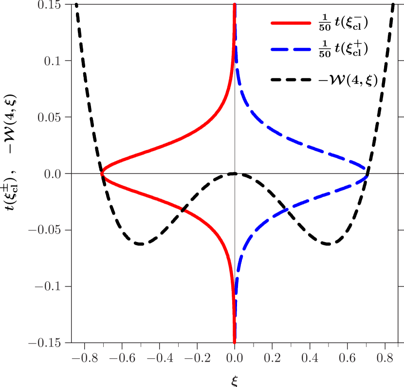
       (a)

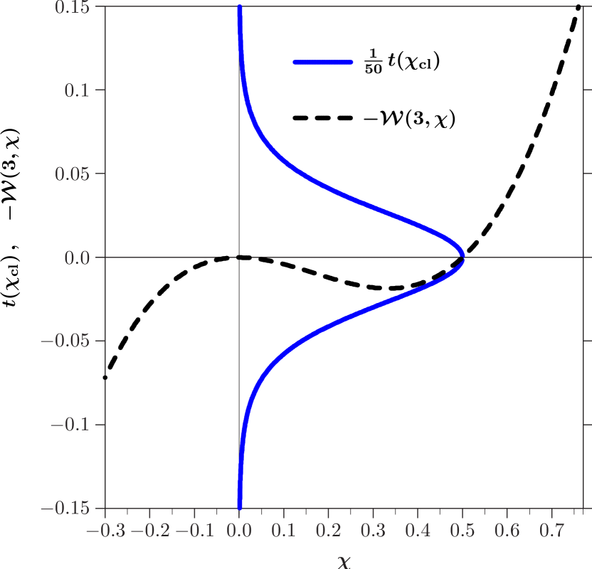
       (b)

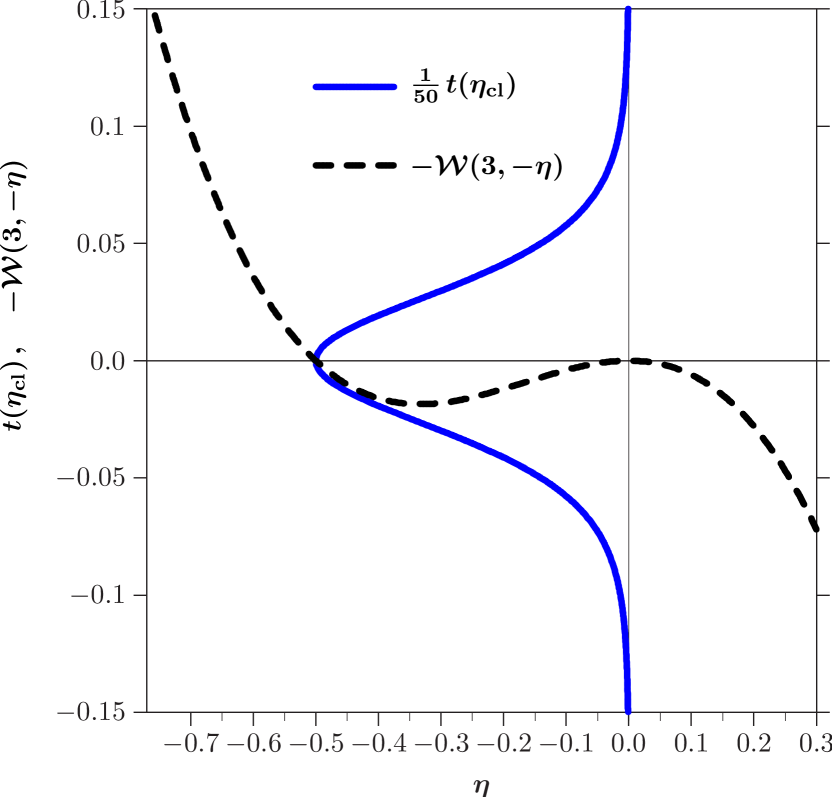
       (c)

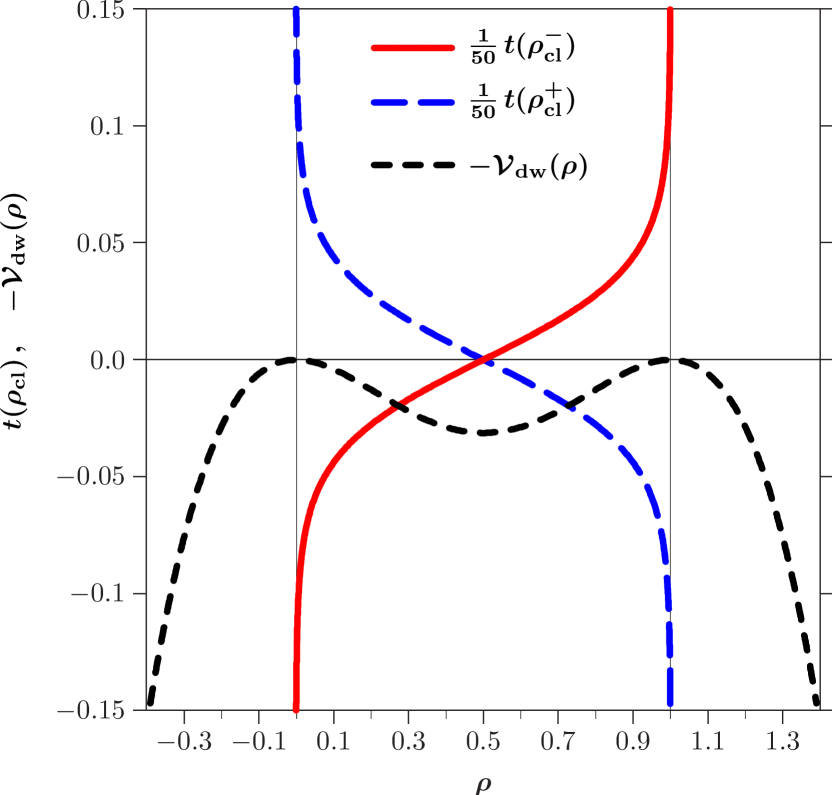
       (d)

Figure 2.1: Trajectories (world lines, the time axis is the ordinate) of several instantons. The quartic ($N=4$) instanton configuration $\chi^{\pm}_{\rm cl}(t)$ is given in Eq. (2.11b) and shown in Fig. (a). The cubic ($M=3$) instanton $\chi_{\rm cl}(t)$ is given in Eq. (2.15b) and shown in Fig. (b). The cubic instanton $\eta_{\rm cl}(t)=-\chi_{\rm cl}(t)$ is found for the reflected cubic potential, where the sign of the $\eta^{3}$ term is inverted [see Eq. (2.20)]. Figure (d) shows the $\rho^{\pm}_{\rm cl}$ instanton which exists for the double-well potential, according to Eq. (2.23).

2.2 Instanton Trajectories

Instantons are nontrivial saddle points of the Euclidean action of a quantum theory, as explained in the first two papers of the current series [1, 2]. The Euclidean action is the action obtained by varying the total energy (kinetic plus potential energy) of a particle along a classical path. The partition function of the anharmonic oscillator can be written as

$$Z(\beta)={\rm Tr}\,\exp(-\beta H)\,,$$ (2.2)

where $H$ is the Hamiltonian of the system [$H=H_{N}(g)$ for an even oscillator, and $H=h_{M}(g)$ for an odd oscillator; in our notation, we suppress the dependence of the right-hand side on the coupling parameter $g$]. A path integral representation of $Z(\beta)$ involves periodic classical orbits,

$${\rm Tr}\,\exp(-\beta\,H)=\int{\mathrm{d}}q_{0}\int\limits_{q\left(-\frac{\beta}{2}\right)=q\left(\frac{\beta}{2}\right)=q_{0}}[{\rm d}q(t)]\,\exp\left\{-{\mbox{\sf{S}}}[-{\textstyle{\frac{1}{2}}}\beta,{\textstyle{\frac{1}{2}}}\beta,q]\right\}\,,$$ (2.3)

where the integration over the end point $q_{0}$ of the classical trajectory (which is equivalent to its starting point) is explicitly given. The Euclidean action ${\mbox{\sf{S}}}[-{\textstyle{\frac{1}{2}}}\beta,{\textstyle{\frac{1}{2}}}\beta,q]$ is the integral over the kinetic and potential energy of the system as it evolves from Euclidean time $-{\textstyle{\frac{1}{2}}}\beta$ to ${\textstyle{\frac{1}{2}}}\beta$. For an even oscillator of degree $N$, we have

$${\mbox{\sf{S}}}_{N}[-{\textstyle{\frac{1}{2}}}\beta,{\textstyle{\frac{1}{2}}}\beta,q]=\int\limits_{-\beta/2}^{\beta/2}{\rm d}t\,\left[\frac{1}{2}\,\left(\dot{q}(t)^{2}+q(t)^{2}\right)+g\,q(t)^{N}\right]\,,$$ (2.4)

whereas for an odd oscillator of degree $M$,

$${\mbox{\sf{s}}}_{M}[-{\textstyle{\frac{1}{2}}}\beta,{\textstyle{\frac{1}{2}}}\beta,q]=\int\limits_{-\beta/2}^{\beta/2}{\rm d}t\,\left[\frac{1}{2}\,\left(\dot{q}(t)^{2}+q(t)^{2}\right)+\sqrt{g}\,q(t)^{M}\right]\,.$$ (2.5)

In order to calculate the perturbative expansion of, say, the ground-state energy of an anharmonic oscillator, one expands about the trivial saddle point of the Euclidean action, which is given by the classical trajectory $q(t)=0$. One writes

$${\mbox{\sf{S}}}_{N}[-{\textstyle{\frac{1}{2}}}\beta,{\textstyle{\frac{1}{2}}}\beta,q]= \;\frac{1}{2}\int\limits_{-\beta/2}^{\beta/2}{\rm d}t\int\limits_{-\beta/2}^{\beta/2}{\rm d}t^{\prime}q(t)\,M(t,t^{\prime})\,q(t^{\prime})+g\int\limits_{-\beta/2}^{\beta/2}{\rm d}t\,q(t)^{N}\,,$$ (2.6a)

$${\mbox{\sf{s}}}_{M}[-{\textstyle{\frac{1}{2}}}\beta,{\textstyle{\frac{1}{2}}}\beta,q]= \;\frac{1}{2}\int\limits_{-\beta/2}^{\beta/2}{\rm d}t\int\limits_{-\beta/2}^{\beta/2}{\rm d}t^{\prime}q(t)\,M(t,t^{\prime})\,q(t^{\prime})+\sqrt{g}\int\limits_{-\beta/2}^{\beta/2}{\rm d}t\,q(t)^{M}\,,$$ (2.6b)

$$M(t,t^{\prime})= \;\delta(t-t^{\prime})\,\left(-\frac{\partial^{2}}{\partial t^{\prime 2}}+1\right)\,.$$ (2.6c)

The inverse of $M$ is the propagator

$$\Delta(t,t^{\prime})=\int\limits_{-\infty}^{\infty}\frac{{\rm d}p}{2\pi}\,\frac{{\rm e}^{{\rm i}\,p\,(t-t^{\prime})}}{p^{2}+1}=\frac{1}{2}\,\exp(-|t-t^{\prime}|)\,.$$ (2.7)

As described in Ref. [35], the perturbative expansion for the ground-state energy

$$E_{0}(g)=\lim_{\beta\to\infty}\left(-\frac{1}{\beta}\,\ln\left({\rm Tr}\,\exp(-\beta\,H)\right)\right)$$ (2.8)

involves Feynman diagrams which can be expressed in terms of integrals of the progagator (2.7). Because the exponentiated [see Eq. (2.2)] quadratic quantum fluctuation about the saddle point given by the $M$ operator in Eq. (2.6) is equivalent to a Gaussian integration measure, one calls the saddle point given by the classical path $q(t)=0$ the Gaussian saddle point.

In view of the obvious dominance of the Gaussian saddle point of the Euclidean action for the perturbative expansion, one might wonder if other nontrivial saddle points exist, and if yes, what role they might play. The Euclidean action corresponding to the path $[q(t)=0]$ is zero. Instantons are classical paths which lead to a finite Euclidean action in the limit of infinite Euclidean time $\beta$. They do not correspond to a physical motion of the particle in the potential under investigation, but rather, to a classical motion in an inverted potential. We remember that the Lagrange function for a classical particle is $T-V$, whereas in the Euclidean action we are integrating over $T+V$ ($T$ is the kinetic energy, and $V$ is the potential).

In order to appreciate the importance of the instanton configurations (which are depicted in Fig. 2.1), we must consider a slightly more complicated situation, namely, the cut of the partition function in the complex plane which is present for “unstable” values of the coupling parameter $g$, i.e., for those which lead to a potential with unstable, relative minima and potential wells through which the particle may tunnel [36, 37]. For the even oscillators as given by the Hamiltonian (2.1a), the unstable coupling parameters are given by $g<0$, because the potential ${\textstyle{\frac{1}{2}}}q^{2}-|g|\,q^{N}$ approaches $-\infty$ for $q\to\pm\infty$. For an odd oscillator [see Eq. (2.1b)], all positive values of $g$ lead to an unstable potential because ${\textstyle{\frac{1}{2}}}q^{2}+g\,q^{M}\to-\infty$ for $q\to-\infty$. The ground-state energy in this case acquires an imaginary part and becomes a resonance energy. The imaginary part of the resonance energy is related to the imaginary part of the partition function according to

$${\mathrm{Im}}E_{0}(g)=\lim_{\beta\to\infty}\left(-\frac{1}{\beta}\,\frac{{\mathrm{Im}}\,Z(\beta)}{Z(\beta)}\right)\,.$$ (2.9)

The sign of the imaginary part of $E_{0}$ depends on the sign of the (infinitesimal) imaginary part of $g$. Discussing (for definiteness) the case of an even oscillator, we define $E_{0}(g)$ to be the resonance energy [with ${\mathrm{Im}}E_{0}(g)<0$] for $g=-|g|+{\mathrm{i}}0$ and to be the anti-resonance energy [with ${\mathrm{Im}}E_{0}(g)>0$] for $g=-|g|-{\mathrm{i}}0$. The cut of the resonance energy then coincides with the cut of the partition function. It has been observed in Refs. [37, 35] that the contribution of the Gaussian saddle point to the cut of the partition function, i.e., to ${\mathrm{Im}}Z(\beta)$, vanishes, and that ${\mathrm{Im}}Z(\beta)$ can be approximated very well by the instanton configurations.

In order to find the instanton configuration for the even oscillator, we scale the classical path as $q(t)=(-g)^{-1/(N-2)}\,\xi(t)$ in Eq. (2.4). The Euclidean action becomes

$${\mbox{\sf{S}}}_{N}=(-g)^{-\frac{2}{N-2}}\,\int{\mathrm{d}}t\,\left({\textstyle{\frac{1}{2}}}\,{\dot{\xi}}^{2}+{\textstyle{\frac{1}{2}}}\,\xi^{2}-\xi^{N}\right)\,.$$ (2.10)

The instanton now is to be searched in the space of the paths $\xi(t)$, whose Euclidean action remains finite when $t$ goes from $-\infty$ to $\infty$. For $N=4$ and $t_{0}=0$, the motion corresponds to a classical trajectory in the inverted potential $\xi^{4}-{\textstyle{\frac{1}{2}}}\xi^{2}$ and is depicted in Fig. 2.1(a). It becomes immediately clear that the instanton configuration is twofold degenerate. Namely, starting for Euclidean time $t\to\infty$ at a position $\xi(t=-\infty)$ infinitesimally to the left or to the right of the central maximum of the inverted potential, the particle may go through either one of the two “troughs” to the right or to left, before bouncing back toward the central maximum at Euclidean time $t\to\infty$. According to Refs. [38, 35], the corresponding solutions to the (Euclidean) equations of motion read, for general $N$,

$$q^{\pm}_{\rm cl}(t)= \;(-g)^{-\frac{2}{N-2}}\,\chi^{\pm}_{\rm cl}(t)\,,$$ (2.11a)

$$\chi^{\pm}_{\rm cl}(t)= \;\pm\frac{1}{\{1+\cosh[(N-2)(t-t_{0})]\}^{1/(N-2)}}\,.$$ (2.11b)

Here, $t_{0}$ is the “starting point” of the instanton, acting as a collective coordinate for the instanton configuration from the point of view of the path integral formalism [35]. The instanton action is

$${\mbox{\sf{S}}}_{N}[q^{\pm}_{\rm cl}]= \;\left(-\frac{2}{g}\right)^{2/(N-2)}\,B\left(\frac{N}{N-2},\frac{N}{N-2}\right)=\left(-\frac{1}{g}\right)^{2/(N-2)}\,{\cal A}(N)\,,$$ (2.12)

$${\cal A}(m)= \;2^{2/(m-2)}\,B\left(\frac{m}{m-2},\frac{m}{m-2}\right)\,,$$ (2.13)

where $B(x,y)=\Gamma(x)\,\Gamma(y)/\Gamma(x+y)$ is the Euler Beta function.

For odd anharmonic oscillators of degree $M$, we transform $q(t)=-g^{-1/(2M-4)}\chi(t)$ and obtain the scaled Euclidean action [cf. Eq. (2.5)]

$${\mbox{\sf{s}}}_{M}=g^{-\frac{1}{M-2}}\,\int{\mathrm{d}}t\,\left({\textstyle{\frac{1}{2}}}\,{\dot{\chi}}^{2}+{\textstyle{\frac{1}{2}}}\,\chi^{2}-\chi^{M}\right)\,.$$ (2.14)

With this scaling, the inverted potential now reads $\chi^{M}-{\textstyle{\frac{1}{2}}}\chi^{2}$ and is of the same form as for the even oscillator. The instanton trajectory $q(t)=q_{\rm cl}(t)$ is unique and reads

$$q_{\rm cl}(t)= \;g^{-\frac{1}{M-2}}\,\chi_{\rm cl}(t)\,,$$ (2.15a)

$$\chi_{\rm cl}(t)= \;\frac{1}{\{1+\cosh[(M-2)(t-t_{0})]\}^{1/(M-2)}}\,.$$ (2.15b)

For the case $M=3$ and $t=t_{0}$, the trajectory is shown in Fig. 2.1(b). Inserting $q_{\rm cl}(t)$ into Eq. (2.14), we obtain the instanton action

$${\mbox{\sf{s}}}_{M}[q_{\rm cl}]= \;\left(\frac{4}{g}\right)^{1/(M-2)}\,B\left(\frac{M}{M-2},\frac{M}{M-2}\right)=\left(\frac{1}{g}\right)^{1/(M-2)}\,{\cal A}(M)\,.$$ (2.16)

Both instanton actions (2.12) and (2.16) are positive in the domain where the instantons exist (for negative coupling in the case of an even oscillator and for positive coupling in the case of an odd oscillator).

The formulas (2.12) and (2.16) can be unified. Namely, if we parameterize the perturbation as $g\,q^{m}$ for general (even or odd) $m$, then we can write the instanton action as $(\mp 2/g)^{2/(m-2)}\,B(\textstyle{\frac{m}{m-2},\frac{m}{m-2}})$, where the plus and minus signs correspond to odd and even potentials, respectively.

The scaled instanton action ${\cal A}(m)$ is expressible in terms of a scaled potential ${\mathcal{W}}(m,q)$ where the sign of the perturbative term has been inverted,

$${\mathcal{W}}(m,q)=\frac{1}{2}\,q^{2}-q^{m}\,.$$ (2.17)

As evident from Fig. 2.1, the instanton configurations correspond to the motion of a classical particle in a potential $-{\mathcal{W}}(m,q)$. We obtain from the paths given in (2.11b) and (2.15b),

$${\cal A}(m)=\int\limits_{0}^{2^{-1/(m-2)}}{\mathrm{d}}q\,\left(2\,\sqrt{2\,{\mathcal{W}}(m,q)}\right)=2^{2/(m-2)}\,B\left(\frac{m}{m-2},\frac{m}{m-2}\right)\,,$$ (2.18)

where we note that $2^{-1/(m-2)}$ is a zero of the potential ${\mathcal{W}}(m,q)$.

The instanton path defined in Eq. (2.15a) fulfills $q_{\rm cl}(t)>0$. However, this instanton configuration is not uniquely associated with the Hamiltonian (2.1b). To see this, we start from an odd anharmonic oscillators of degree $M$ and transform $q(t)=g^{-1/(2M-4)}\,\eta(t)$. In this manner, we obtain the scaled Euclidean action [cf. Eq. (2.5)]

$${\mbox{\sf{s}}}_{M}=g^{-\frac{1}{M-2}}\,\int{\mathrm{d}}t\,\left({\textstyle{\frac{1}{2}}}\,{\dot{\eta}}^{2}+{\textstyle{\frac{1}{2}}}\,\eta^{2}+\eta^{M}\right)\,.$$ (2.19)

With this scaling, the inverted potential reads $-\left(\eta^{M}+{\textstyle{\frac{1}{2}}}\,\eta^{2}\right)=\left(-\eta\right)^{M}-{\textstyle{\frac{1}{2}}}\,\eta^{2}$. By comparison to Eq. (2.15b), the instanton is found to be

$$\eta_{\rm cl}(t)=-\frac{1}{\{1+\cosh[(M-2)(t-t_{0})]\}^{1/(M-2)}}<0\,.$$ (2.20)

For $M=3$ and $t_{0}=0$, the corresponding instanton trajectory is shown in Fig. 2.1(c).

For the double-well potential, the Euclidean action reads, according to Eq. (2.10a) of Ref. [1],

$${\mbox{\sf{S}}}_{\rm dw}=\int{\mathrm{d}}t\,\left(\frac{1}{2}\,{\dot{\rho}}^{2}+\frac{1}{2g^{2}}\,\rho^{2}(1-\rho)^{2}\right)\,.$$ (2.21)

This expression contains the double-well potential

$${\cal V}_{\rm dw}(q)=\frac{1}{2}\,\rho^{2}(1-\rho)^{2}\,.$$ (2.22)

One of the possible instanton configurations is

$$\rho^{+}_{\rm cl}(t)=\left(\exp\left[\frac{t-t_{0}}{g}\right]+1\right)^{-1}\,,$$ (2.23a)

where again $$t_{0} t=-\infty t=\infty \rho^{+}_{\rm cl}(t) \rho^{-}_{\rm cl}(t)$$ is a collective coordinate. The instanton configuration joins the two minima of the double-well potential. It does not define a periodic path whose starting point at is the same as the end point at . In order to construct a periodic orbit, one has to “join” two instantons according to Fig. 5 of Sec. 4.4.1 of Ref. [1], so that the pseudoparticle returns to its initial point. This can be done by joining the instanton trajectory with the trajectory , where

$$\rho^{-}_{\rm cl}(t)=\left(\exp\left[\frac{t_{0}-t}{g}\right]+1\right)^{-1}\,,$$ (2.23b)

which is shown in Fig. 2.1(d), for the case $t_{0}=0$. The instanton action is found to be

$${\mbox{\sf{S}}}_{\rm dw}[\rho^{\pm}_{\rm cl}]=\frac{1}{6\,g}\,.$$ (2.24)

Let us recall an important difference of the odd oscillators (and of the double well, by the way) to the even oscillators. In the former cases, the instanton configuration is found for all positive, real values of the coupling parameter. In the latter case (even oscillator), one first has to scale the action to be consistent with the case of negative coupling [see Eq. (2.10)], before solving for the instanton [see Eq. (2.15b) and Fig. 2.1(a)]. For the even oscillator, the instanton only exists for specific regions in the space of complex coupling constants.

2.3 Quantum Fluctuations and Decay Widths

According to Refs. [37, 35], the quantum fluctuations about the instanton configurations give rise to a functional determinant of a Bargmann potential, whose spectrum and determinant are analytically calculable. For the ground state of an even oscillator, this calculation leads to the result

$${\rm Im}\,E_{0}^{(N)}(g)\;\mathop{\sim}^{g\to 0^{-}}\;-\frac{1}{\sqrt{2\pi}}\,\left(\frac{2{\mathcal{C}}(N)}{(-g)^{2/(N-2)}}\right)^{1/2}\exp\left(-\frac{{\cal A}(N)}{(-g)^{2/(N-2)}}\right)\,,$$ (2.25)

where

$${\cal C}(m)=\frac{1}{2^{2/(m-2)}}\,\exp\left[\;\int\limits_{0}^{2^{-1/(m-2)}}{\mathrm{d}}q\,\left(\frac{\sqrt{2}}{\sqrt{{\mathcal{W}}(m,q)}}-\frac{2}{q}\right)\right]=\;2^{2/(m-2)}\,.$$ (2.26)

A slight generalization of this result to the $n$th resonance energy $E_{n}^{(N)}(g)$, for potentials of even order $N$, leads to

$${\rm Im}\,E_{n}^{(N)}(g)\;\mathop{\sim}^{g\to 0^{-}}\;-\frac{1}{n!\sqrt{2\pi}}\,\left(\frac{2{\mathcal{C}}(N)}{(-g)^{2/(N-2)}}\right)^{n+1/2}\exp\left(-\frac{{\cal A}(N)}{(-g)^{2/(N-2)}}\right)\,.$$ (2.27)

We take the opportunity to correct a misprint in Eq. (8) of Ref. [3], where the sign of the mantissa of the exponent $n+1/2$ was accidentally inverted. This result is valid in leading order; corrections are of relative order $g^{2/(N-2)}$. For odd potentials in the normalization given by Eq. (2.1b) and for positive coupling, we have for $g\to 0$,

$${\rm Im}\,\epsilon_{0}^{(M)}(g)\;\mathop{\sim}^{g\to 0^{+}}\;-\frac{1}{2\sqrt{2\pi}}\,\left(\frac{2{\mathcal{C}}(M)}{g^{1/(M-2)}}\right)^{1/2}\,\exp\left(-\frac{{\cal A}(M)}{g^{1/(M-2)}}\right)\,.$$ (2.28)

The generalization to arbitrary $n$ reads

$${\rm Im}\,\epsilon_{n}^{(M)}(g)\;\mathop{\sim}^{g\to 0^{+}}\;-\frac{1}{2n!\sqrt{2\pi}}\,\left(\frac{2{\mathcal{C}}(M)}{g^{1/(M-2)}}\right)^{n+1/2}\,\exp\left(-\frac{{\cal A}(M)}{g^{1/(M-2)}}\right)\,.$$ (2.29)

The sign of the imaginary parts of the resonance energies in Eqs. (2.25), (2.27), (2.28) and (2.29) is negative, as it should be for a resonance energy (as opposed to an anti-resonance, where the imaginary part of the energy is positive). As outlined in Refs. [37, 35], the sign of the imaginary part of the energy is somewhat arbitrary as it is determined by the square root $\sqrt{e_{0}}=\pm{\mathrm{i}}|\sqrt{e_{0}}|$, where $e_{0}<0$ is the (only) negative eigenvalue of the matrix that describes the quantum fluctuations about the instanton configurations. As we see in the following, the resonance energies $E_{n}^{(N)}(g)$ and $\epsilon_{n}^{(M)}(g)$ actually have cuts along the negative and the positive real $g$ axis, respectively. We have to associate either sign of the imaginary part with a particular side of the branch cut. This becomes clear when we discuss the dispersion relations fulfilled by the resonance energies.

2.4 Dispersion Relations

The dispersion relations formulate connections of the values of the resonance energies $E_{n}^{(N)}(g)$ and $\epsilon_{n}^{(M)}(g)$ of the even and odd oscillators as a function of $g$ in the complex $g$ plane. Before we discuss them, let us first justify the use of the convention $\sqrt{g}\,q^{M}$ for the perturbative term in the odd oscillator of degree $M$ [see Eq. (2.1b)]. The dispersion relation for odd oscillators is intimately linked with the square-root convention for the coupling term.

For illustrative purposes, we consider the Hamiltonian in the normalization $h_{M}(g)=-{\textstyle{\frac{1}{2}}}\partial_{q}^{2}+{\textstyle{\frac{1}{2}}}q^{2}+\sqrt{g}\,q^{M}$, with odd $M$. A change in the sign of the coupling term $\sqrt{g}\to-\sqrt{g}$ can be compensated by a parity transformation $q\to-q$. So, if $\psi(q)$ is a resonance eigenfunction of the cubic Hamiltonian, suitably continued into the complex plane, then $\psi(-q)$ is a resonance eigenfunction for the cubic Hamiltonian with a sign change of $\sqrt{g}$, but the same resonance eigenvalue. We conclude that the resonance spectrum of the cubic Hamiltonian is invariant under the transformation $\sqrt{g}\to-\sqrt{g}$.

It is thus natural to formulate the cubic Hamiltonian as a function of $\sqrt{g}$, because once $g$ is specified, the ambiguity in defining the square root is absorbed into the invariance of the resonance spectrum of the Hamiltonian under a sign change of the coupling term. A specification of $g$ alone suffices to define the spectrum of resonances. As a function of $g$, the resonance eigenvalues of $h_{M}(g)$ have branch cuts along the positive real axis. For $g={\rm Re}(g)+{\rm i}\,0$, the imaginary parts are negative, whereas for $g={\rm Re}(g)-{\rm i}\,0$, the imaginary parts are positive. For negative coupling $g=-|g|<0$, the resonance eigenvalues of $h_{3}(g)$,

$$h_{3}(-|g|)=-\frac{1}{2}\,\partial_{q}^{2}+\frac{1}{2}\,q^{2}\pm{\mathrm{i}}|g|^{1/2}\,q^{3}\,,\quad g>0,$$ (2.30)

have no imaginary part at all because the cubic Hamiltonian is ${\mathcal{P}T}$-symmetric for imaginary coupling and has a purely real spectrum. Therefore the only branch cut of the resonance eigenvalues of the cubic Hamiltonian is along the positive real axis. Note that the ${\mathcal{P}T}$-symmetry of the cubic Hamiltonian here serves as a property which facilitates our analysis of the structure of the branch cuts.

In general, the dispersion relation [14] for the resonance energy eigenvalues $\epsilon^{(M)}_{m}(g)$ of a general odd oscillator therefore reads

$$\epsilon_{n}^{(M)}(g)=n+\frac{1}{2}+\frac{g}{\pi}\,\int\limits_{0}^{\infty}{\mathrm{d}}s\,\frac{{\rm Im}\,\epsilon_{n}^{(M)}(s+{\rm i}\,0)}{s\,(s-g)}\,.$$ (2.31a)

The subtracted dispersion relation [39, 20, 6] for the energies $$E_{n}(N,g) N$$ of the even anharmonic oscillators of degree is

$$E^{(N)}_{n}(g)=n+\frac{1}{2}-\frac{g}{\pi}\,\int\limits_{-\infty}^{0}{\rm d}s\,\frac{{\rm Im}\,E^{(N)}_{n}(s+{\rm i}\,0)}{s\,(s-g)}\,.$$ (2.31b)

These are subtracted dispersion relations; the term $n+{\textstyle{\frac{1}{2}}}$ fixes the energy level for vanishing coupling.

2.5 Generalized Bender–Wu Formulas

The general expressions for the imaginary parts of the resonance energies given in Eqs. (2.27) and (2.29), together with the dispersion relations (2.31a) and (2.31b), can be used in order to derive integral representations for the perturbative coefficients and to derive their leading factorial growth for large orders of perturbation theory. Based on Eq. (2.31b), we can expand the integrand in powers of $g$, and obtain the coefficients of the perturbation series for the energy levels of an even oscillator. We find for the $n$th level of the oscillator of order $N$,

$$E^{(N)}_{n}(g)\sim\sum_{K=0}^{\infty}E^{(N)}_{n,K}\,g^{K}\,,\qquad E^{(N)}_{n,K\geq 1}=-\frac{1}{\pi}\,\int\limits_{-\infty}^{0}{\rm d}s\,\frac{{\rm Im}\,E^{(N)}_{n}(s+{\rm i}\,0)}{s^{K+1}}\,.$$ (2.32a)

Because $${\rm Im}\,E^{(N)}_{n}(s+{\rm i}\,0)<0 -\infty<s<0 s (-1)^{K+1} K\geq 1 n M$$ for and because the integration variable is negative along the entire integration contour, the sign of the perturbative coefficients is determined according to the formula for . By contrast, for the th level of an odd anharmonic oscillator of degree , we have

$$\epsilon^{(M)}_{n}(g)\sim\sum_{K=0}^{\infty}\epsilon^{(M)}_{n,K}\,g^{K}\,,\qquad\epsilon^{(M)}_{n,K\geq 1}=\frac{1}{\pi}\,\int\limits_{0}^{\infty}{\rm d}s\,\frac{{\rm Im}\,\epsilon^{(M)}_{n}(s+{\rm i}\,0)}{s^{K+1}}\,.$$ (2.32b)

We can again argue that ${\rm Im}\,\epsilon^{(M)}_{n}(s+{\rm i}\,0)<0$ for $0<s<\infty$, i.e. along the entire integration contour. This implies that the perturbative coefficients for the odd anharmonic oscillators are all negative, except for the zeroth-order term (in $g$), which is simply $n+{\textstyle{\frac{1}{2}}}$.

Based on Eq. (2.27) and (2.31b), it is a simple matter of integration to calculate the large-order perturbative expansion for an arbitrary level of an even oscillator of arbitrary degree,

$$E_{n,K}^{(N)}\sim \;\frac{(-1)^{K+1}\,(N-2)}{\pi^{3/2}\,n!\,2^{K+1-n}}\;\Gamma\left(\frac{N-2}{2}K+n+{\textstyle{\frac{1}{2}}}\right)\left[B\left(\frac{N}{N-2},\frac{N}{N-2}\right)\right]^{-\frac{N-2}{2}K-n-{\textstyle{\frac{1}{2}}}}\,,\quad K\to\infty,$$ (2.33)

which is valid up to corrections of relative order $K^{-1}$. We here confirm the result of Bender and Wu [20]. Our new result concerns the case of odd oscillators, where we integrate (2.31b) using Eqs. (2.29) and find

$$\epsilon^{(M)}_{n,K}\sim \;\frac{2-M}{\pi^{3/2}\,n!\,2^{2K+1-n}}\;\Gamma\left((M-2)K+n+{\textstyle{\frac{1}{2}}}\right)\left[B\left(\frac{M}{M-2},\frac{M}{M-2}\right)\right]^{-(M-2)K-n-{\textstyle{\frac{1}{2}}}}\,,\quad K\to\infty.$$ (2.34)

The formulas for the $K$th order perturbative coefficients $E_{n,K}^{(N)}$ and $\epsilon^{(M)}_{n,K}$ have been compared to numerical calculations for a number of example cases, as discussed below in Sec. 4.

Chapter 3 From WKB Expansions to Generalized Quantization Conditions

 

3.1 Perturbative Expansion

The approach outlined in Sec. 2 is inspired by field-theoretical considerations and leads to an intuitive understanding of the physics involved in the derivation of the leading-order factorial growth of the perturbative coefficients, as given in Eqs. (2.33) and (2.34). However, this formalism does not make use of the additional simple structure of the problem at hand, namely, the structure of a one-dimensional nonrelativistic quantum mechanical oscillator for which semiclassical or Wentzel–Kramers–Brioullin (WKB) and perturbative expansions can be derived without any further technical difficulties. Here, we strive to combine both methods in order to derive higher-order formulas which grant us access to phenomenologically relevant, numerically large correction terms.

To this end, we first investigate the derivation of higher-order perturbative approximants to the wave functions and to the energy eigenvalues of the anharmonic oscillators. Suitable scaling transformations in the original Schrödinger equation corresponding to the Hamiltonians (2.1a) and (2.1b) prove useful in that regard. For the even oscillator given by Eq. (2.1a), we start from

$$\left(-\frac{1}{2}\,\frac{\partial^{2}}{\partial q^{2}}+\frac{1}{2}\,q^{2}+g\,q^{N}\right)\,\varphi=E\,\varphi$$ (3.1)

and transform according to $q\to g^{-1/(N-2)}\,q$, which leads to

$$\left(-\frac{g^{\frac{4}{N-2}}}{2}\,\frac{\partial}{\partial q^{2}}+\frac{1}{2}\,q^{2}+q^{N}\right)\,\varphi=g^{\frac{2}{N-2}}\,E\,\varphi\,.$$ (3.2)

For (2.1b), we start from

$$\left(-\frac{1}{2}\,\frac{\partial^{2}}{\partial q^{2}}+\frac{1}{2}\,q^{2}+\sqrt{g}\,q^{M}\right)\,\varphi=E\,\varphi$$ (3.3)

and transform according to $q\to g^{-1/(2(M-2))}\,q$

$$\left(-\frac{g^{\frac{2}{M-2}}}{2}\,\frac{\partial}{\partial q^{2}}+\frac{1}{2}\,q^{2}+q^{M}\right)\,\varphi=g^{\frac{1}{M-2}}\,E\,\varphi\,.$$ (3.4)

We identify the general coupling parameter

$${G}\equiv{G}(m,g)=g^{X(m)}\,,\qquad X(m)={\frac{2[\mkern-2.5mu[m/2]\mkern-2.5mu]-m+2}{m-2}}\,,$$ (3.5)

which implies that ${G}(M,g)=g^{1/(M-2)}$ for odd $M$ and ${G}(N,g)=g^{2/(N-2)}$ for even $N$ (here, $[\mkern-2.5mu[X]\mkern-2.5mu]$ is the largest integer smaller than $X$). With this identification, Eqs. (3.2) and (3.4) have the general structure

$$\left(-\frac{1}{2}\,{G}^{2}\,\frac{\partial}{\partial q^{2}}+{\mathcal{V}}(m,q)\right)\,\varphi={G}\,E\,\varphi\,,$$

$${\mathcal{V}}(m,q)=\frac{1}{2}\,q^{2}+q^{m}\,.$$ (3.6)

Note that the potential ${\mathcal{V}}(m,q)$ differs from the potential ${\mathcal{W}}(m,q)$ used for the calculation of the instanton configurations, in the sign of the $q^{m}$ term [for the definition of ${\mathcal{W}}(m,q)$, see Eq. (2.17)].

Using the scaled and unified form for the Schrödinger equation given by Eq. (3.1), the wave functions and resonance energies are amenable to a perturbative treatment. The general formalism has been outlined in Sec. 3 of Ref. [2] and is recalled here, with a special emphasis on the anharmonic oscillators. We first transform the Schrödinger equation to the Riccati equation by setting

$$\frac{\varphi^{\prime}(q)}{\varphi(q)}=-\frac{s(q)}{{G}}\,,\qquad\frac{\varphi^{\prime\prime}(q)}{\varphi(q)}=\frac{s^{2}(q)}{{G}^{2}}-\frac{s^{\prime}(q)}{{G}}\,,$$ (3.7)

The Riccati form of the Schrödinger equation then reads,

$${G}\,s^{\prime}(q)-s^{2}(q)+{\mathcal{U}}^{2}(q)=0\,,$$ (3.8a)

$${\mathcal{U}}(q)=\sqrt{2\left[\,{\mathcal{V}}(m,q)-{G}\,E\,\right]}\,.$$ (3.8b)

The coupling $G$ formally takes the role of $\hbar$ in the scaled equation. The function $S(q)$ is proportional to the logarithmic derivative of the wave function. It has an implicit dependence on the degree $m$ of the oscillator, on the coupling ${G}$ and on the energy $E$, which we suppress in our notation. We can uniquely decompose $S(q)$ into even-parity and odd-parity (in ${G}$) components,

$$s(q)= \;s_{+}(q)+s_{-}(q)=s_{+}(m,q,E,{G})+s_{-}(m,q,E,{G})\,,$$ (3.9a)

where

$$s_{\pm}(m,q,-{G},-E)=\pm s_{\pm}(m,q,{G},E)\,.$$ (3.9b)

This leads to the following system of equations,

$${G}\,s^{\prime}_{-}(q)-s_{+}(q)^{2}-s_{-}(q)^{2}+{\mathcal{U}}^{2}(q)= \;0\,,$$ (3.10a)

$${G}\,s^{\prime}_{+}(q)-2\,s_{+}(q)\,s_{-}(q)= \;0\,.$$ (3.10b)

From the second of these equations, we have

$$s_{-}(q)=\frac{{G}}{2}\,\frac{s^{\prime}_{+}(q)}{s_{+}(q)}\,,$$ (3.11)

so that we can write $s$ as a function of $s_{+}$ only. By virtue of the decomposition (3.9), this means that

$$\varphi(q)=\frac{1}{\sqrt{s_{+}(q)}}\,\exp\left(-{G}^{-1}\,\int{\mathrm{d}}q\,s_{+}(q)\right)\,.$$ (3.12)

If we approximate $s(q)\approx s_{+}(q)\approx\sqrt{2{\mathcal{V}}(m,q)}$, then this is just the textbook version of the Wentzel–Kramers–Brioullin (WKB) approximation [40]. The advantage of the above formalism is that it allows for systematic expansions both for fixed $E$ in powers of ${G}$, which leads to the perturbative expansion of the energy levels, but also in powers of ${G}$ at ${G}\,E$ fixed, which is an expansion relevant a priori for excited states, because ${G}$ is assumed to be small and $E$ must be large for ${G}\,E$ to attain values of order unity. The latter approach leads to the WKB expansion.

We start, though, with the perturbative expansion. Because the wave function for the $n$th excited state has $n$ zeros on the real line, we can formulate the following quantization condition,

$$\frac{1}{2\pi{\mathrm{i}}}\,\oint_{C}{\mathrm{d}}z\,\frac{\varphi^{\prime}(z)}{\varphi(z)}=-\frac{1}{2\pi{\mathrm{i}}\,{G}}\,\oint_{C}{\mathrm{d}}z\,s(z)=n\,,$$ (3.13)

where $C$ is a contour that encloses all the zeros in the counterclockwise (mathematically positive) direction and the definition in Eq. (3.7) for the logarithmic derivative of the wave function has been used. Equation (3.13) is the Bohr–Sommerfeld quantization condition.

We now seek a solution of Eq. (3.10) by expansion in ${G}$ at $E$ fixed, taking advantage of the elimination of $s_{-}(q)$ via (3.10b). It is easy to see that the solutions for $s(q)$ and $s_{+}(q)$ can be written in terms of the expression

$${u}(q)=\sqrt{2\,{\mathcal{V}}(m,q)}$$ (3.14)

alone. Furthermore, the zeros of the denominators of $S(q)$ and $S_{+}(q)$ are given exclusively by the zero(s) of ${u}(q)$. Because of the simple structure of the Riccati equation (3.8), one can write a recursive scheme, within the perturbative expansion in powers of $g$ at fixed $E$, that leads to higher-order perturbative approximants which we would like to label by a lowercase $s$,

$$s(q)= \;\sum_{K=0}^{\infty}{G}^{K}\,s_{K}(q)\,,\qquad s_{0}(q)={u}(q)\,,\qquad s_{1}(q)=\frac{{u}^{\prime}(q)-2E}{2{u}(q)}\,,$$

$$s_{K}(q)= \;\frac{1}{2\,{u}(q)}\left(s^{\prime}_{K-1}(q)-\sum_{l=1}^{K-1}s_{K-l}(q)\,s_{l}(q)\right)\,,\qquad K\geq 2.$$ (3.15)

To order ${G}^{2}$, we find for the symmetric part $s_{+}(q)$ which is invariant under the exchange $g\to-g$, $E\to-E$,

$$s_{+}(q)= \;{u}(q)-G\,\frac{E}{{u}(q)}+{G}^{2}\,\left(\frac{1}{4}\,\frac{{u}^{\prime\prime}(q)}{{u}^{2}(q)}-\frac{3}{8}\,\frac{{u}^{\prime}(q)^{2}}{{u}^{3}(q)}-\frac{1}{2}\,\frac{E^{2}}{{u}^{3}(q)}\right)+{\mathcal{O}}({G}^{3})\,.$$ (3.16)

This structure implies that the only location relevant for the singularities in the contour integral (3.13) is the origin in the complex $z$-plane. For even anharmonic oscillators, this is immediately obvious because the only zero of the function $u(q)=q\,\sqrt{1+2q^{N}}$ then lies on the real axis ($N$ even). For odd anharmonic oscillators, the function $u(q)=q\,\sqrt{1+2q^{M}}$ has an additional zero on the real axis at $x_{M}=-2^{1/M}$. However, the residue at $x_{M}$ vanishes.

Because $s_{-}(q)={\textstyle{\frac{1}{2}}}\,{G}\,s^{\prime}_{+}(q)/s_{+}(q)$ and $s(q)=s_{+}(q)+s_{-}(q)$, we can finally write the quantization condition (3.13) as

$$-\frac{1}{2\pi{\mathrm{i}}\,{G}}\,\oint_{C}{\mathrm{d}}z\,s_{+}(z)=n+\frac{1}{2}\,.$$ (3.17)

Here, $C$ is a contour that encloses only the origin. The advantage of this formalism is that the function $B(m,E,{G})$, defined by

$$B(m,E,{G})\equiv-\frac{1}{2\pi{\mathrm{i}}\,{G}}\,\oint_{C}{\mathrm{d}}z\,s_{+}(z)\,,$$ (3.18)

provides for a universal means of determining the perturbative expansion for an arbitrary excited level, by means of the perturbative quantization condition

$$B(m,E,{G})=n+\frac{1}{2}\,.$$ (3.19)

The rational is to construct higher-order approximants to the wave function according to Eq. (3.1), then to find the residue of the higher-order approximants to the wave function at the origin. The sum of the residues of the higher-order (in $G$) terms then defines the function $B(m,E,{G})$.

3.2 Example: Perturbative Expansion of the Sextic Potential

The generalized coupling parameter for the sextic potential with $N=6$ is given by Eq. (3.5) as $G=g^{1/2}$. The zeroth-order approximant is

$$s_{0}(q)=u(q)=q\,\sqrt{1+2q^{4}}\,.$$ (3.20)

Entering into the recursive system (3.1) and calculating the residue at $q=0$, we obtain

$$B(6,E,G)= \;E-G^{2}\left(\frac{25}{8}\,E+\frac{5}{2}\,E^{3}\right)$$

$$\;+G^{4}\,\left(\frac{21777}{256}\,E+\frac{5145}{32}\,E^{3}+\frac{693}{16}\,E^{5}\right)+{\mathcal{O}}(G^{6})$$

$$= \;E-g\left(\frac{25}{8}\,E+\frac{5}{2}\,E^{3}\right)$$

$$\;+g\,\left(\frac{21777}{256}\,E+\frac{5145}{32}\,E^{3}+\frac{693}{16}\,E^{5}\right)+{\mathcal{O}}(g^{3})$$ (3.21)

Note, in particular, that the term $-E/u(q)$ in Eq. (3.16) leads to the leading term $E+{\mathcal{O}}(G^{2})$ in Eq. (3.2) in view of $u(q)=q+{\mathcal{O}}(q^{4})$. Note also that the term of order $G$ in Eq. (3.16) does not produce any contributions to the residue at the origin. By explicitly solving the equation $B(6,E_{0}^{(6)},G)={\textstyle{\frac{1}{2}}}$ for the ground state resonance energy $E_{0}^{(6)}$ order by order in $G^{2}=g$, one obtains the perturbative expansion (as a function of $g$),

$$E_{0}^{(6)}= \;\frac{1}{2}+\frac{15}{8}\,G^{2}-\frac{3495}{64}\,G^{4}+{\mathcal{O}}(G^{6})$$

$$= \;\frac{1}{2}+\frac{15}{8}\,g-\frac{3495}{64}\,g^{2}+{\mathcal{O}}(g^{3})\,,$$ (3.22)

for the ground state of the sextic potential.

3.3 Semiclassical or WKB Expansion

We now turn our attention to the WKB expansion, which is an expansion in powers of $G$ for fixed $G\,E$. A priori, a natural starting point for the WKB expansion would be Eq. (3.8b), with $S(q)\approx{\mathcal{U}}(q)=\sqrt{2\,{\mathcal{V}}(m,q)-2\,{G}\,E}$. However, a second purpose of our construction of the WKB expansion is the calculation of the instanton action, and of perturbations thereof. We have already seen in Sec. 2 that the instanton configuration does not exist for arbitrary values of the coupling parameter. In the case of an even oscillator, it exists only for negative coupling $g<0$ [see Fig. 2.1(a)]. In the case of an odd oscillator, the instanton configuration involves positive values of the coordinates only if we assume that $\sqrt{g}<0$ [see Fig. 2.1(b)]. For $\sqrt{g}>0$, the instanton configuration entails negative values of the coordinate [see Fig. 2.1(c)]. We therefore have to scale the coupling constants differently as compared to Sec. 3.1, if we wish to grasp the instanton configuration within our semiclassical expansion.

Let us start with the case of an even oscillator, with $g=-|g|<0$. Starting from [see Eq. (2.1a)], we obtain

$$\left(-\frac{1}{2}\,\frac{\partial^{2}}{\partial q^{2}}+\frac{1}{2}\,q^{2}-|g|\,q^{N}\right)\,\phi=E\,\phi$$ (3.23)

and transform according to $q\to|g|^{-1/(N-2)}\,q$, which leads to

$$\left(-\frac{|g|^{\frac{4}{N-2}}}{2}\,\frac{\partial}{\partial q^{2}}+\frac{1}{2}\,q^{2}-q^{N}\right)\,\phi=|g|^{\frac{2}{N-2}}\,E\,\phi\,.$$ (3.24)

The sign of the $q^{N}$ term is inverted as compared to Eq. (3.2). For an odd oscillator, we start from

$$\left(-\frac{1}{2}\,\frac{\partial^{2}}{\partial q^{2}}+\frac{1}{2}\,q^{2}+\sqrt{g}\,q^{M}\right)\,\phi=E\,\phi$$ (3.25)

and transform according to $q\to-g^{-1/[2(M-2)]}\,q$, which gives

$$\left(-\frac{g^{\frac{2}{M-2}}}{2}\,\frac{\partial}{\partial q^{2}}+\frac{1}{2}\,q^{2}-q^{M}\right)\,\phi=g^{\frac{1}{M-2}}\,E\,\phi\,.$$ (3.26)

We define the general coupling parameter

$$\widetilde{G}\equiv\widetilde{G}(m,g)=|g|^{X(m)}\,,\qquad X(m)={\frac{2[\mkern-2.5mu[m/2]\mkern-2.5mu]-m+2}{m-2}}\,,$$ (3.27)

where $X(m)$ is given in Eq. (3.5). With this identification, Eqs. (3.24) and (3.26) have the general structure

$$\left(-\frac{1}{2}\,\widetilde{G}^{2}\,\frac{\partial}{\partial q^{2}}+{\mathcal{W}}(m,q)\right)\,\varphi=\widetilde{G}\,E\,\varphi\,,$$

$${\mathcal{W}}(m,q)=\frac{1}{2}\,q^{2}-q^{m}\,.$$ (3.28)

Here, we reencounter the potential ${\mathcal{W}}(m,q)$ where the sign of the $q^{m}$ term is inverted as compared to ${\mathcal{V}}(m,q)$. We set

$$\frac{\phi^{\prime}}{\phi}=-\frac{{\mathrm{S}}(q)}{\widetilde{G}}\,,$$ (3.29)

where the symbol ${\mathrm{S}}$ (as compared to $S$) denotes the logarithmic derivative of the scaled wave function for the potential ${\mathcal{W}}(m,q)$. The Riccati form of the Schrödinger equation then reads, in terms of ${\mathrm{S}}$,

$$\widetilde{G}\,{\mathrm{S}}^{\prime}(q)-{\mathrm{S}}^{2}(q)+{\mathcal{T}}^{2}(q)=0\,,$$ (3.30a)

$${\mathcal{T}}(q)=\sqrt{2\left[\,{\mathcal{W}}(m,q)-\widetilde{G}\,E\,\right]}\,.$$ (3.30b)

The recursive scheme for calculating higher-order WKB approximants then reads

$${\mathrm{S}}(q)= \;\sum_{K=0}^{\infty}\widetilde{G}^{K}\,{\mathrm{S}}_{K}(q)\,,\qquad{\mathrm{S}}_{0}(q)={\mathcal{T}}(q)\,,\qquad{\mathrm{S}}_{1}(q)=\frac{{\mathrm{S}}_{0}^{\prime}(q)}{2\,{\mathrm{S}}_{0}(q)}\,,$$

$${\mathrm{S}}_{K}(q)= \;\frac{1}{2\,{\mathrm{S}}_{0}(q)}\left({\mathrm{S}}^{\prime}_{K-1}(q)-\sum_{l=1}^{K-1}{\mathrm{S}}_{K-l}(q)\,{\mathrm{S}}_{l}(q)\right)\,.$$ (3.31)

Unlike the perturbative approximants, which have an isolated pole at $q=0$, the WKB approximants have a branch cut, which coincides with the branch cut of the square root function of the zeroth-order WKB expansion,

$${\mathrm{S}}_{0}(q)=\sqrt{2\left[\,{\mathcal{W}}(m,q)-\widetilde{G}\,E\,\right]}\,.$$ (3.32)

In practical calculations, it turns out to be convenient to define the square root function so that its branch cut is along the positive real axis (this aspect will be discussed below).

Let us here recall the perturbative quantization condition derived for the perturbative approximant $s_{+}(z)$ as given above in Eqs. (3.17) and (3.18),

$$\frac{1}{{G}}\,\oint_{C}{\mathrm{d}}z\,s_{+}(z)=-2\pi{\mathrm{i}}\,B(m,E,{G})=-2\pi{\mathrm{i}}\,\left(n+\frac{1}{2}\right)\,.$$ (3.33)

Here, $C$ was defined as a contour that encircles all poles of $s_{+}(z)$ on the real axis in the mathematically positive sense.

These correspond to the perturbative functions at a particular value of ${G}$. In order to make the connection to the formalism given above, we must therefore identify the particular value of $\widetilde{G}$ that corresponds to the same value of the original coupling parameter $g$ as the value of $\widetilde{G}$ we are using for our calculations.

For even potentials, this identification proceeds as follows. We have

$$G=g^{2/(N-2)}$$ (3.34)

and $\widetilde{G}$, for negative $g$, is given by

$$\widetilde{G}=|g|^{2/(N-2)}=(-g)^{2/(N-2)}\,,\qquad g<0\,,$$ (3.35)

so that

$$\widetilde{G}=\left(-{G}^{(N-2)/2}\right)^{2/(N-2)}=\exp\left(\frac{2\pi{\mathrm{i}}}{N-2}\right)\,{G}=\left(-g\right)^{2/(N-2)}\,,$$ (3.36)

on the cut, i.e. for $g<0$. For odd $M$, we have

$${G}=g^{1/(M-2)}$$ (3.37)

and

$$\widetilde{G}=|g|^{1/(M-2)}=g^{1/(M-2)}\,,\qquad g>0\,,$$ (3.38)

so that

$$\widetilde{G}={G}=g^{1/(M-2)}\,.$$ (3.39)

We thus have

$$\widetilde{G}=\exp[{\mathrm{i}}\,\Phi(m)]\;G\,,\qquad\Phi(m)=\left\{\begin{array}[]{cc}\displaystyle{\frac{2\pi}{m-2}}&\qquad\mbox{$m$ even}\\[1.29167pt] 1&\qquad\mbox{$m$ odd}\end{array}\right.\,.$$ (3.40)

Consequently, it appears useful to consider the contour integral of the WKB expansion around its cut,

$$\frac{1}{\widetilde{G}}\,\oint_{{\mathcal{C}}}{\mathrm{d}}z\,{\mathrm{S}}_{+}(z)\,,$$ (3.41)

where ${\mathcal{C}}$ is a contour that encircles the cut of the WKB expansion in the mathematically negative, clockwise sense, and $S_{+}(z)$ is the part of the WKB approximation $S(z)$ that is symmetric under the transformation $g\to-g$, $E\to-E$. Namely, in analogy to (3.9), we define the decomposition

$${\mathrm{S}}(q)= \;{\mathrm{S}}_{+}(q)+{\mathrm{S}}_{-}(q)={\mathrm{S}}_{+}(m,q,E,{G})+{\mathrm{S}}_{-}(m,q,E,{G})\,,$$ (3.42a)

where

$${\mathrm{S}}_{\pm}(m,q,-E,-{G})=\pm\,{\mathrm{S}}_{\pm}(m,q,E,{G})\,.$$ (3.42b)

The contour integral about the cut of the function ${\mathrm{S}}_{+}$ leads to a more complex structure as compared to the right-hand side of Eq. (3.17),

$$\frac{1}{\widetilde{G}}\;\oint\limits_{{\mathcal{C}}}{\mathrm{d}}z\,{\mathrm{S}}_{+}(q)=A(m,E,G)+{\textstyle{\frac{1}{2}}}\ln(2\pi)-\ln\left[\Gamma\left({\textstyle{\frac{1}{2}}}-B(m,E,{G})\right)\right]+B(m,E,{G})\,\ln\left(-\frac{\widetilde{G}}{2\,{\mathcal{C}}(m)}\right)\,.$$ (3.43)

The left-hand side of the above equation is calculated as a function of $\widetilde{G}$, a priori [including the WKB approximation to the wave function, ${\mathrm{S}}(q)$]. The right-hand side defines, implicitly, functions of ${G}$. The procedure is to calculate the integral of ${\mathrm{S}}_{+}(q)$ about the cut, first of all, as a function of $\widetilde{G}$,

$$f(\widetilde{G})=\frac{1}{\widetilde{G}}\;\oint\limits_{{\mathcal{C}}}{\mathrm{d}}z\,{\mathrm{S}}_{+}(q)\,,$$ (3.44)

and then to identify

$$f(\widetilde{G})=f\left(\Phi(m)\,{G}\right)=A(m,E,G)+{\textstyle{\frac{1}{2}}}\ln(2\pi)$$

$$\qquad-\ln\left[\Gamma\left({\textstyle{\frac{1}{2}}}-B(m,E,{G})\right)\right]+B(m,E,{G})\,\ln\left(-\frac{\exp[{\mathrm{i}}\,\Phi(m)]\;{G}}{2\,{\mathcal{C}}(m)}\right)\,.$$ (3.45)

Let us analyze the right-hand side of Eq. (3.3). To this end, we expand the expression $\ln\left[\Gamma\left({\textstyle{\frac{1}{2}}}-B(m,E,{G})\right)\right]$ for large principal quantum numbers. Because

$$\ln\Gamma({\textstyle{\frac{1}{2}}}+z)\approx z\,\ln(z)-z\,,$$ (3.46)

and in view of

$$B(m,E,{G})=E+{\mathcal{O}}(G)\,,$$ (3.47)

we can approximate the logarithmic terms on the right-hand side of (3.3) as follows. Taking only the first term from Eq. (3.46), we obtain

$$-\ln\Gamma\left({\textstyle{\frac{1}{2}}}-B(m,E,{G})\right)+B(m,E,{G})\,\ln\left(-\frac{\widetilde{G}}{2\,{\mathcal{C}}(m)}\right)$$

$$\qquad\approx B(m,E,{G})\,\ln(-E)+B(m,E,{G})\,\ln\left(-\frac{\widetilde{G}}{2\,{\mathcal{C}}(m)}\right)\approx B(m,E,{G})\,\ln\left(\frac{\widetilde{G}{}\,E}{2\,{\mathcal{C}}(m)}\right)\,.$$ (3.48)

This expression is real if $\widetilde{G}$ is positive (if $E$ is real). However, if the arguments of both logarithms in the second line of the above equation acquire an infinitesimal negative imaginary part, then both logarithms acquire an imaginary part of $\pm\pi i$, and the term $2\pi{\mathrm{i}}B(m,E,{G})$, previously encountered the right-hand side of Eq. (3.33), is recovered, thus establishing a connection of the WKB and the perturbative contour integrals.

The strategy now is to calculate the contour integral in Eq. (3.44) and then to use the already determined result for the function $B(m,E,{G})$ (see Sec. 3.1 of the current work) to subtract perturbative terms from the right-hand side of Eq. (3.3), in order to obtain subsequently higher-order terms of the function $A(m,E,G)$ in the WKB limit ${G}\to 0$ and ${G}\,E$ fixed. A well-defined analytic procedure for the evaluation of the contour integral in Eq. (3.44), based on the method of asymptotic matching (see Sec. 7.4 of Ref. [41]), is presented below in Sec. 3.4. In leading order, one can show that

$$A(m,E,G)\approx\frac{{\cal A}(m)}{\widetilde{G}}=\left\{\begin{array}[]{cc}\displaystyle{\frac{{\cal A}(m)}{(-g)^{2/(m-2)}}}&\qquad\mbox{$m$ even}\\[1.29167pt] \displaystyle{\frac{{\cal A}(m)}{g^{1/(m-2)}}}&\qquad\mbox{$m$ odd}\end{array}\right.\,,$$ (3.49)

where ${\cal A}(m)$ is the instanton action defined in Eq. (2.18). We will therefore call $A(m,E,G)$ the instanton function in the current article.

At the end of the calculation, it is thus natural to reexpress the “perturbative $B$ function” and the “instanton $A$ function” in terms of the original coupling $g$ given in Eqs. (2.1a) and (2.1b). We thus define

$$A_{m}(E,g)= \;A(m,E,g^{\frac{2[\mkern-2.5mu[m/2]\mkern-2.5mu]-m+2}{m-2}})\,,$$ (3.50a)

$$B_{m}(E,g)= \;B(m,E,g^{\frac{2[\mkern-2.5mu[m/2]\mkern-2.5mu]-m+2}{m-2}})\,.$$ (3.50b)

In this convention, the $B_{m}$ functions have an argument of integer power (just $g$) and contain also only integer powers of the coupling in their expansion in $g$. The $A_{m}$ functions, though, contain fractional powers except for the oscillators of the third, the fourth, and the sixth degree (the latter one is a special case).

3.4 Example: Contour Integrals for the Quartic Potential

We remember that the contour integral around the cut of the WKB expansion is to be evaluated for the case where instantons persist, i.e., for $g<0$. We have $N=4$ and therefore, in view of Eqs. (3.5) and (3.27),

$$\widetilde{G}=-G=-g\qquad\qquad\mbox{$(N=4)$\,.}$$ (3.51)

The task is to evaluate the contour integral of the symmetric part ${\mathrm{S}}_{+}(q)$ of the WKB expansion of the logarithmic derivative of the wave function, as defined in Eq. (3.41). We approximate

$$T= \;\frac{1}{\widetilde{G}}\oint\limits_{\cal C}{\mathrm{d}}q\,{\mathrm{S}}_{+}(q)\approx-\frac{1}{g}\oint\limits_{\cal C}{\mathrm{d}}q\,\left[{\mathrm{S}}_{0}(q)+g^{2}\,{\mathrm{S}}_{2}(q)+g^{4}\,{\mathrm{S}}_{4}(q)\right]=T_{0}+T_{2}+T_{4}\,.$$ (3.52)

Here, the WKB approximants ${\mathrm{S}}_{0}(q)$, ${\mathrm{S}}_{2}(q)$ and ${\mathrm{S}}_{4}(q)$ are defined in Eq. (3.3), and the integrals $T_{0}$, $T_{2}$ and $T_{4}$ are defined in the obvious manner. One can easily show that the contributions from the terms ${\mathrm{S}}_{1}(q)$ and ${\mathrm{S}}_{3}(q)$ vanish, and we recall that ${\mathcal{C}}$ is a contour that encircles the cut of the WKB expansion in the clockwise direction. The zeroth-order term is

$$T_{0}=-\frac{1}{g}\oint\limits_{\cal C}{\mathrm{d}}q\;{\mathrm{S}}_{0}(q)\,,$$ (3.53)

with the zeroth-order WKB approximant

$${\mathrm{S}}_{0}(q)=\sqrt{2{\mathcal{W}}(4,q)-\widetilde{G}E}=\sqrt{q^{2}-2q^{4}+gE}\,.$$ (3.54)

We define the square root function to have its branch cut along the positive real axis. Directly above the cut, the value of the square root is positive, while directly below, it is negative. As the contour is clockwise, we thus have an integration interval from zero to $1/\sqrt{2}$, while below the real axis, we go from $1/\sqrt{2}$ to zero. With this definition, the contour integral is

$$T_{0}=-\frac{1}{g}\oint\limits_{\cal C}{\mathrm{d}}q\,\sqrt{q^{2}-2q^{4}+gE}=-\frac{2}{g}\,{\mathrm{Re}}\int\limits_{0}^{{\textstyle{\frac{1}{\sqrt{2}}}}}{\mathrm{d}}q\,(q^{2}-2q^{4}+gE)^{1/2}\,.$$ (3.55)

The specification of the real part is necessary because we evaluate the contour integral about the cut of of the WKB expansion. For the evaluation, we use the method of asymptotic matching (see Ch. 7.4 of Ref. [41]) which involves an overlapping parameter $\epsilon$, that is also used in Lamb shift calculations [42, 43, 44] in order to separate the low-energy from the high-energy contribution to the bound-electron self-energy. The overlapping parameter fulfills

$$0\ll g\,E\ll\epsilon\,,$$ (3.56)

and we divide the integration interval $(0,1/\sqrt{2})$ into three parts, which are the intervals $(0,\epsilon)$, $(\epsilon,{\textstyle{\frac{1}{\sqrt{2}}}}-\epsilon)$, and $({\textstyle{\frac{1}{\sqrt{2}}}}-\epsilon,1/\sqrt{2})$. Each result is first expanded in $g\,E$, then in $\epsilon$, and the divergent terms in $\epsilon$ cancel at the end of the calculation. We remember that the integral is evaluated for $g<0$. The integral $T_{0}$ is recovered as

$$T_{0}=-\frac{2}{g}\,\left(I_{1}+I_{2}+I_{3}\right)\,,$$ (3.57)

where the $I_{j}$ comprise the above mentioned three intervals, respectively. The first contribution is, up to order $(g\,E)^{4}$,

$$I_{1}= \;{\mathrm{Re}}\int\limits_{0}^{\epsilon}{\mathrm{d}}q\,(q^{2}-2q^{4}+gE)^{1/2}$$

$$= \;(gE)\,\left[\frac{1}{2}+\frac{1}{2}\,\ln\left(\frac{2\epsilon^{2}}{gE}\right)\right]+(gE)^{2}\,\left[\frac{7}{8}+\frac{1}{4\epsilon^{2}}-\frac{3}{4}\,\ln\left(-\frac{2\epsilon^{2}}{gE}\right)\right]$$

$$\;+(gE)^{3}\,\left[-\frac{319}{48}-\frac{1}{8\epsilon^{4}}-\frac{5}{4\epsilon^{2}}+\frac{35}{8}\,\ln\left(-\frac{2\epsilon^{2}}{gE}\right)\right]$$

$$\;+(gE)^{4}\,\left[\frac{23189}{384}+\frac{5}{48\epsilon^{6}}+\frac{35}{32\epsilon^{4}}+\frac{315}{32\epsilon^{2}}-\frac{1155}{32}\,\ln\left(-\frac{2\epsilon^{2}}{gE}\right)\right]\,.$$ (3.58)

Here, we have taken into account the fact that only the real part of the result matters; hence, the argument of the logarithms reads $-2\epsilon^{2}/(gE)>0$, because $g<0$. The second interval leads to

$$I_{2}= \;{\mathrm{Re}}\int\limits_{\epsilon}^{{\textstyle{\frac{1}{\sqrt{2}}}}-\epsilon}{\mathrm{d}}q\,(q^{2}-2q^{4}+gE)^{1/2}$$

$$= \;\frac{1}{6}+(gE)\,\left[\frac{1}{2}\,\ln\left(\frac{2}{\epsilon^{2}}\right)\right]+(gE)^{2}\,\left[\frac{5}{4}-\frac{1}{4\epsilon^{2}}-\frac{1}{2^{3/4}\epsilon^{1/2}}-\frac{3}{4}\,\ln\left(\frac{2}{\epsilon^{2}}\right)\right]$$

$$\;+(gE)^{3}\,\left[-\frac{319}{48}+\frac{1}{8\epsilon^{4}}+\frac{5}{4\epsilon^{2}}+\frac{1}{6\,2^{1/4}\epsilon^{3/2}}+\frac{25}{4\,2^{3/4}\epsilon^{1/2}}+\frac{35}{8}\,\ln\left(\frac{2}{\epsilon^{2}}\right)\right]$$

$$\;+(gE)^{4}\,\left[\frac{13327}{192}-\frac{5}{48\epsilon^{6}}-\frac{35}{32\epsilon^{4}}-\frac{315}{32\epsilon^{2}}\right.$$

$$\;\qquad\left.-\frac{1}{8\,2^{3/4}\epsilon^{5/2}}-\frac{175}{96\,2^{1/4}\epsilon^{3/2}}-\frac{6755}{128\,2^{3/4}\epsilon^{1/2}}-\frac{1155}{32}\,\ln\left(\frac{2}{\epsilon^{2}}\right)\right]\,.$$ (3.59)

The third interval gives rise to the following results,

$$I_{3}={\mathrm{Re}}\int\limits_{{\textstyle{\frac{1}{\sqrt{2}}}}-\epsilon}^{{\textstyle{\frac{1}{\sqrt{2}}}}}{\mathrm{d}}q\,(q^{2}-2q^{4}+gE)^{1/2}=(gE)^{2}\,\left[\frac{1}{2^{3/4}\epsilon^{1/2}}\right]+(gE)^{3}\,\left[-\frac{1}{6\,2^{1/4}\epsilon^{3/2}}\right.$$

$$\quad\left.-\frac{25}{4\,2^{3/4}\epsilon^{1/2}}\right]+(gE)^{4}\,\left[\frac{1}{8\,2^{3/4}\epsilon^{5/2}}+\frac{175}{96\,2^{1/4}\epsilon^{3/2}}+\frac{6755}{128\,2^{3/4}\epsilon^{1/2}}\right]\,.$$ (3.60)

Terms that originate from the upper limit of integration in the third interval are expressed in terms of half-integer powers of $g\,E$. These terms (an example is $(g\,E)^{7/2}=(g\,E)^{3}\,\sqrt{g\,E}$ involve the square root of negative argument because $g\,E<0$ and are thus imaginary (hence, they do not contribute to the real part of the result). We have defined the square root to have its branch cut along the negative real axis, and so the contributions from the upper and lower branch of the contour ${\mathcal{C}}$ cancel for these terms. Finally, after the cancellation of $\epsilon$, $T_{0}$ is found as

$$T_{0}=-\frac{1}{3g}+\left\{-E+E\,\ln\left(-\frac{gE}{4}\right)\right\}+g\,\left[-\frac{17}{4}E^{2}-\frac{3}{2}\,E^{2}\,\ln\left(-\frac{gE}{4}\right)\right]$$

$$+g^{2}\,\left[\frac{59}{2}E^{3}+\frac{35}{4}\,E^{3}\,\ln\left(-\frac{gE}{4}\right)\right]+g^{3}\,\left[-\frac{49843}{192}E^{4}-\frac{1155}{16}\,E^{4}\,\ln\left(-\frac{gE}{4}\right)\right]\,.$$ (3.61)

For the second term,

$$T_{2}=-g\oint\limits_{\cal C}{\mathrm{d}}q\,{\mathrm{S}}_{2}(q)\,,$$ (3.62)

we find

$$T_{2}=-\frac{1}{24\,E}+g\,\left[-\frac{35}{24}-\frac{3}{8}\,\ln\left(-\frac{gE}{4}\right)\right]$$

$$+g^{2}\,\left[\frac{2093}{96}E+\frac{85}{16}\,E\,\ln\left(-\frac{gE}{4}\right)\right]+g^{3}\,\left[-\frac{16285}{48}E^{2}-\frac{2625}{32}\,E^{2}\,\ln\left(-\frac{gE}{4}\right)\right]\,.$$ (3.63)

The third term is

$$T_{4}=-g^{3}\oint\limits_{\cal C}{\mathrm{d}}q\,{\mathrm{S}}_{4}(q)\,,$$ (3.64)

with

$$T_{4}=\frac{7}{2880\,E^{3}}-\frac{3\,g}{640\,E^{2}}+\frac{821\,g^{2}}{3840\,E}+g^{3}\,\left[-\frac{205621}{4608}-\frac{1995}{256}\ln\left(-\frac{gE}{4}\right)\right]\,.$$ (3.65)

The total result of the contour integral of the WKB expansion is $T=T_{0}+T_{2}+T_{4}$, where

$$T=\frac{7}{2880\,E^{3}}-\frac{1}{24\,E}-\frac{1}{3g}+\left\{-E+E\,\ln\left(-\frac{gE}{4}\right)\right\}$$

$$+g\,\left[-\frac{3}{640\,E^{2}}-\frac{35}{24}-\frac{17}{4}E^{2}+\left(-\frac{3}{8}-\frac{3}{2}\,E^{2}\right)\,\ln\left(-\frac{gE}{4}\right)\right]$$

$$+g^{2}\,\left[\frac{821}{3840\,E}+\frac{2093}{96}E+\frac{59}{2}\,E^{3}+\left(\frac{85}{16}E+\frac{35}{4}\,E^{3}\right)\,\ln\left(-\frac{gE}{4}\right)\right]$$

$$+g^{3}\,\left[-\frac{205621}{4608}-\frac{16285}{48}E^{2}-\frac{49843}{192}E^{4}+\left(-\frac{1995}{256}-\frac{2625}{32}\,E^{2}-\frac{1155}{16}E^{4}\right)\,\ln\left(-\frac{gE}{4}\right)\right]\,.$$ (3.66)

The perturbative counterterms read

$$P={\textstyle{\frac{1}{2}}}\ln(2\pi)-\ln\left[\Gamma\left({\textstyle{\frac{1}{2}}}-B_{4}(E,g)\right)\right]+B_{4}(E,g)\,\ln\left(\frac{g}{4}\right)$$

$$=\frac{7}{2880\,E^{3}}-\frac{1}{24\,E}+\left\{-E+E\,\ln\left(-\frac{gE}{4}\right)\right\}$$

$$+g\,\left[-\frac{3\,g}{640\,E^{2}}-\frac{1}{16}+\left(-\frac{3}{8}-\frac{3}{2}\,E^{2}\right)\,\ln\left(-\frac{gE}{4}\right)\right]$$

$$+g^{2}\,\left[\frac{821}{3840\,E}+\frac{5}{6}E+\frac{9}{8}\,E^{3}+\left(\frac{85}{16}E+\frac{35}{4}\,E^{3}\right)\,\ln\left(-\frac{gE}{4}\right)\right]$$

$$+g^{3}\,\left[-\frac{4349}{1024}-\frac{1649}{128}E^{2}-\frac{201}{16}E^{4}+\left(-\frac{1995}{256}-\frac{2625}{32}\,E^{2}-\frac{1155}{16}E^{4}\right)\,\ln\left(-\frac{gE}{4}\right)\right]\,,$$ (3.67)

where the result [for the definition of $B_{4}(E,g)$, see Eq. (3.50)]

$$B_{4}(E,g)= \;B(4,E,g)=E-g\left(\frac{3}{8}+\frac{3}{2}\,E^{2}\right)+g^{2}\,\left(\frac{85}{16}\,E+\frac{35}{4}\,E^{3}\right)$$

$$\;-\,g^{3}\,\left(\frac{1995}{256}+\frac{2625}{32}\,E^{2}+\frac{1155}{16}\,E^{4}\right)$$ (3.68)

has been used, as well as the asymptotic expansion

$$\ln\Gamma({\textstyle{\frac{1}{2}}}+z)=z\,\left\{\ln(z)-1\right\}+{\textstyle{\frac{1}{2}}}\ln(2\pi)-\frac{1}{24\,z}+\frac{7}{2880\,z^{3}}+\dots\,.$$ (3.69)

Note that the logarithmic term $E\,\ln(-gE/4)$ in the perturbative counterterms [Eq. (3.4)] is obtained after combining the term $-\ln\Gamma(1/2-B_{4}(E,g))\approx E\,\ln(-E)$ with the term $B_{4}(E,g)\ln(g/4)\approx E\,\ln(g/4)$. The instanton function $A_{4}(E,g)$ for the quartic potential is finally found to read

$$A_{4}(E,g)=T-P=-\frac{1}{3\,g}+g\,\left(-\frac{67}{48}-\frac{17}{4}E^{2}\right)+g^{2}\,\left(\frac{671}{32}\,E+\frac{227}{8}E^{3}\right)$$

$$\qquad+g^{3}\,\left(-\frac{372101}{9216}-\frac{125333}{384}E^{2}-\frac{47431}{192}E^{4}\right)+{\mathcal{O}}(g^{4})\,.$$ (3.70)

We finally remark that in all intermediate expressions (3.52)—(3.4), we have neglected higher-order terms that contribute in the order $g^{4}$ and higher to the function $A_{4}(E,g)$. The term of order $g^{4}$ can be found below in Eq. (4.11).

Alternative methods for the evaluation of the contour integrals about the cut of the WKB expansion are described in Appendix F of Ref. [2]. One of these is based on a Mellin transformation with respect to $E$, after which the $q$ integral can be performed with ease, followed by a Mellin backtransformation, which evaluates the original integrals. The second alternative method is an adaptation of dimensional regularization and is described in Appendix F.7 of Ref. [2]. The method described above, which directly evaluates the integrals along contours infinitesimally displaced from the real axis, might be most transparent one among the various approaches, and therefore we have chosen it in the current context for illustrative purposes.

3.5 Generalized Quantization Conditions

In Sec. 3.1, we have investigated the perturbative expansion for the logarithmic derivative of the wave function. The perturbative quantization condition $B_{m}(E,g)=n+{\textstyle{\frac{1}{2}}}$ was derived for an oscillator of degree $m$, where $m$ can be either even or odd [see Eqs. (3.19) and (3.50)]. For the “stable” configurations which concern even potentials with positive coupling and odd potentials with imaginary coupling ${\rm Re}\,g=0$, there are no nontrivial saddle points of the Euclidean action, and thus no instanton configurations to consider. The quantization conditions are thus equal to the perturbative condition, and read

$$B_{N}(E,g)= \;n+{\textstyle{\frac{1}{2}}}\,,\qquad\mbox{$N$ even}\,,\qquad g>0\,,$$ (3.71a)

$$B_{M}(E,g)= \;n+{\textstyle{\frac{1}{2}}}\,,\qquad\mbox{$M$ odd}\,,\qquad g<0\,.$$ (3.71b)

The question then is how to modify these conditions for those values of the coupling constant where instanton configurations become relevant. To this end, let us first observe that we can write the conditions as

$$\frac{1}{\Gamma({\textstyle{\frac{1}{2}}}-B_{m}(E,g))}=0\,,$$ (3.72)

where $m$ can be either even or odd. So, on the one hand, according to Eq. (3.47), we have $B_{m}(E,g)=E+{\mathcal{O}}(g)$. On the other hand, the quantity $1/\Gamma({\textstyle{\frac{1}{2}}}-E)$ can naturally be identified as the spectral determinant of the harmonic oscillator with Hamiltonian

$${\cal H}=-\frac{1}{2}\,\frac{\partial^{2}}{\partial q^{2}}+\frac{1}{2}\,q^{2}\,.$$ (3.73)

In this form, we naturally identify

$$\frac{1}{\Gamma({\textstyle{\frac{1}{2}}}-E)}={\rm det}({\cal H}-E)$$ (3.74)

as the spectral determinant. The effect of the instanton is to add an infinitesimal imaginary part to the energy of the bound state,

$$E\approx{\cal E}\equiv n+{\textstyle{\frac{1}{2}}}+{\mathrm{i}}\,{\mathrm{Im}}\,{\cal E}\,.$$ (3.75)

Expanding in the nonperturbatively small (in $g$) imaginary part of the energy, we obtain

$$\frac{1}{\Gamma({\textstyle{\frac{1}{2}}}-{\cal E})}\approx-(-1)^{n+1/2}\;n!\;{\mathrm{Im}}\,{\cal E}$$ (3.76)

Now, starting with an even oscillator (for definiteness), the imaginary part of the energy can be approximated as [see Eq. (2.27)]

$${\mathrm{Im}}\,{\cal E}\approx \;{\mathrm{Im}}\,E_{n}^{(N)}(g)\approx-\frac{1}{n!\sqrt{2\pi}}\,\left(\frac{2\,{\mathcal{C}}(N)}{(-g)^{2/(N-2)}}\right)^{n+1/2}\exp\left(-\frac{{\cal A}(N)}{(-g)^{2/(N-2)}}\right)$$

$$\approx \;-\frac{1}{n!\sqrt{2\pi}}\,\left(\frac{2\,{\mathcal{C}}(N)}{(-g)^{2/(N-2)}}\right)^{B_{N}(E,g)}\exp\left(-A_{N}(E,g)\right)\,,$$ (3.77)

we have used (3.49). If we now generalize the left-hand side of Eq. (3.76) as $1/\Gamma({\textstyle{\frac{1}{2}}}-B_{N}(E,g))$ and approximate the right-hand side of Eq. (3.76) by the right-hand side of Eq. (3.5), we have

$$\frac{1}{\Gamma\left({\textstyle{\frac{1}{2}}}-B_{N}(E,g)\right)}=\frac{1}{\sqrt{2\pi}}\,\left(-\frac{2\,{\cal C}(N)}{(-g)^{2/(N-2)}}\right)^{B_{N}(E,g)}\,\exp\left(-A_{N}(E,g)\right)\,,$$

$$\mbox{$N$ even}\,,\qquad g<0\,,$$ (3.78)

which is our conjecture for even oscillators in the “unstable” regime of negative coupling parameter $g<0$.

For an odd oscillator, we approximate the right-hand side of Eq. (3.76) as

$${\mathrm{Im}}\,{\cal E}\approx \;{\rm Im}\,\epsilon_{n}^{(M)}(g)\approx-\frac{1}{n!\sqrt{8\pi}}\,\left(\frac{2\,{\mathcal{C}}(M)}{g^{1/(M-2)}}\right)^{n+1/2}\,\exp\left(-\frac{{\cal A}(M)}{g^{1/(M-2)}}\right)$$

$$\approx \;-\frac{1}{n!\sqrt{8\pi}}\,\left(\frac{2\,{\mathcal{C}}(M)}{g^{1/(M-2)}}\right)^{B_{M}(E,g)}\,\exp\left(-A_{M}(E,g)\right)\,.$$ (3.79)

We now generalize the left-hand side of Eq. (3.76) as $1/\Gamma({\textstyle{\frac{1}{2}}}-B_{M}(E,g))$ and approximate the right-hand side of Eq. (3.76) by the right-hand side of Eq. (3.5), and obtain

$$\frac{1}{\Gamma\left({\textstyle{\frac{1}{2}}}-B_{M}(E,g)\right)}=\frac{1}{\sqrt{8\pi}}\,\left(-\frac{2\,{\cal C}(M)}{g^{1/(M-2)}}\right)^{B_{M}(E,g)}\,\exp[-A_{M}(E,g)]\,,$$

$$\mbox{$M$ odd}\,,\qquad g>0\,,$$ (3.80)

which is our conjecture for odd oscillators in the “unstable” regime of positive coupling parameter $g>0$. In writing Eq. (3.5), we correct a typographical error in Eq. (18b) of Ref. [3], which concerns the missing minus sign in the expression $\left(-\frac{2\,{\cal C}(M)}{g^{1/(M-2)}}\right)^{B_{M}(E,g)}$. The quantization conditions (3.5) and (3.5) effectively assign specific numerical constants to the expression on the right-hand side of Eq. (3.43).

3.6 Generalized Perturbative Expansions

We intend to investigate the structure of generalized perturbative expansions which fulfill the quantization conditions (3.5) and (3.5). To this end, we enter into the quantization conditions (3.5) and (3.5) with an ansatz that involves an unperturbed energy of the form $n+{\textstyle{\frac{1}{2}}}+\eta$ where $\eta$ is a nonperturbatively small imaginary part that is assumed to be composed of a nonperturbative exponential factor, multiplied by fractional powers of the coupling constant. We then expand the $\Gamma$ functions in Eqs. (3.5) and (3.5) about their poles and equate the coefficients of the fractional-power terms. In this manner, we easily derive the following expressions for the decay width of an arbitrary state of an even or odd anharmonic oscillator. We thereby recover the results given here in Eqs. (2.27) and (2.29), but we are able to qualify the order of the relative correction terms. They read

$${\rm Im}\,E_{n}^{(N)}(g<0)= \;-\frac{1}{n!\sqrt{2\pi}}\,\left(\frac{2{\cal C}(N)}{(-g)^{2/(N-2)}}\right)^{n+{\textstyle{\frac{1}{2}}}}\,\exp\left(-\frac{{\cal A}(N)}{(-g)^{2/(N-2)}}\right)$$

$$\;\times\left[1+{\mathcal{O}}(g^{2/(N-2)})\right]$$

$$= \;-\frac{1}{\sqrt{\pi}\,n!}\,\frac{2^{(n\,N+1)/(N-2)}}{(-g)^{(2n+1)/(N-2)}}\,\exp\left(-\frac{2^{2/(N-2)}\,B(\frac{N}{N-2},\frac{N}{N-2})}{(-g)^{2/(N-2)}}\right)\,$$

$$\;\times\left[1+{\mathcal{O}}(g^{2/(N-2)})\right]\,,$$ (3.81a)

for even oscillators, and for odd oscillators, we obtain

$${\rm Im}\,\epsilon_{n}^{(M)}(g>0)= \;-\frac{1}{n!\,\sqrt{8\pi}}\,\left(\frac{2{\cal C}(M)}{g^{1/(M-2)}}\right)^{n+{\textstyle{\frac{1}{2}}}}\,\exp\left(-\frac{{\cal A}(M)}{g^{1/(M-2)}}\right)$$

$$\;\times\left[1+{\mathcal{O}}(g^{1/(M-2)})\right]\,$$

$$= \;-\frac{1}{\sqrt{\pi}\,n!}\,\frac{2^{[(n-1)\,M+3]/(M-2)}}{g^{(2n+1)/(2\,M-4)}}\,\exp\left(-\frac{2^{2/(M-2)}\,B(\frac{M}{M-2},\frac{M}{M-2})}{g^{1/(M-2)}}\right)$$

$$\;\times\left[1+{\mathcal{O}}(g^{1/(M-2)})\right]\,.$$ (3.81b)

Using the dispersion relation (2.31b), we recover the result from Eq. (2.33) for the leading asymptotics for the perturbative coefficients of an arbitrary state $n$ of an even oscillator of degree $N$,

$$E_{n,K}^{(N)}\sim \;\frac{(-1)^{K+1}\,(N-2)}{\pi^{3/2}\,n!\,2^{K+1-n}}\,\left[B\left(\frac{N}{N-2},\frac{N}{N-2}\right)\right]^{-(N-2)\,K/2-n-1/2}$$

$$\;\times\Gamma\left(\frac{N-2}{2}\,K+n+\frac{1}{2}\right)\left[1+{\mathcal{O}}\left(\frac{1}{K}\right)\right]\,,$$ (3.82a)

and clarify that the correction terms are of relative order $$1/K n M$$. The analogous, general result for an arbitrary state of an odd oscillator of degree reads [see Eq. (2.34), we again clarify the order of the correction terms],

$$\epsilon_{n,K}^{(M)}\sim \;-\frac{M-2}{\pi^{3/2}\,n!\,2^{2K+1-n}}\,\left[B\left(\frac{M}{M-2},\frac{M}{M-2}\right)\right]^{-(M-2)\,K-n-1/2}$$

$$\;\times\Gamma\left[(M-2)\,K+n+\frac{1}{2}\right]\,\left[1+{\mathcal{O}}\left(\frac{1}{K}\right)\right]\,.$$ (3.82b)

The quantization condition (3.5) implies the following general structure for the generalized non-analytic expansion (sometimes called “resurgent expansion”) characterizing the resonance energy of the $n$th level of the $N$th anharmonic oscillator (even $N$),

$$E_{n}^{(N)}(g<0)=\sum_{J=0}^{\infty}\left[\frac{{\mathrm{i}}}{n!\sqrt{2\pi}}\,\left(\frac{2{\cal C}(N)}{(-g)^{2/(N-2)}}\right)^{n+{\textstyle{\frac{1}{2}}}}\,\exp\left(-\frac{{\cal A}(N)}{(-g)^{2/(N-2)}}\right)\right]^{J}$$

$$\;\times\sum_{L=0}^{L_{\mathrm{max}}}\,\ln^{L}\left(-\frac{2{\mathcal{C}}(N)}{(-g)^{2/(N-2)}}\right)\sum_{K=0}^{\infty}\Xi^{(N,n)}_{J,L,K}\,(-g)^{2K/(N-2)}$$

$$= \;\sum_{J=0}^{\infty}\left[\frac{{\mathrm{i}}}{\sqrt{\pi}\,n!}\,\frac{2^{(n\,N+1)/(N-2)}}{(-g)^{(2n+1)/(N-2)}}\,\exp\left(-\frac{2^{2/(N-2)}\,B(\frac{N}{N-2},\frac{N}{N-2})}{(-g)^{2/(N-2)}}\right)\right]^{J}$$

$$\;\times\sum_{L=0}^{L_{\mathrm{max}}}\,\ln^{L}\left(-\frac{2^{N/(N-2)}}{(-g)^{2/(N-2)}}\right)\sum_{K=0}^{\infty}\Xi^{(N,n)}_{J,L,K}\,(-g)^{2K/(N-2)}\,,$$ (3.83)

with constant coefficients $\Xi^{(N,n)}_{JLK}$ and $L_{\mathrm{max}}\equiv\mathrm{max}(0,J-1)$. The above triple expansion is complicated and in need of an interpretation. The term with $J=0$ recovers the basic, perturbative expansion which has only integer powers in $g$. Therefore, $\Xi^{(N,n)}_{0,0,K(N-2)/2}=(-1)^{K}\,E^{(N)}_{n,K}$ where the $E^{(N)}_{n,K}$ represent the perturbative coefficients from Eq. (2.32). Note that the perturbative contribution to the energy levels is present for both positive and negative coupling $g$. The term with $J=1$ recovers the leading contribution in the expansion in powers of $\exp(-{\mathcal{A}}(N)/g)$ to the imaginary part of the resonance energy. The term with $J=2$ involves a logarithm of the form $\ln\left(-\frac{2{\mathcal{C}}(N)}{(-g)^{2/(N-2)}}\right)$. The explicit imaginary parts of the logarithms cancel against the imaginary parts of lower-order perturbation series which are summed in complex directions, in a manner consistent with the analytic continuation of the logarithm [45, 46, 47, 2].

Let us illustrate the expansion (3.6) by calculating the first terms in the expansion in powers of $J$ up to $J=3$, including the logarithmic terms, but only up to leading order in $g$, i.e. only the terms with $K=0$, for the ground state of the quartic oscillator. The result of this calculation is

$$E_{0}^{(4)}(g<0)=\left\{\frac{1}{2}+{\mathcal{O}}(g)\right\}-{\mathrm{i}}\,\sqrt{-\frac{2}{\pi\,g}}\,\exp\left(\frac{1}{3\,g}\right)\,\left[1+{\mathcal{O}}(g)\right]$$

$$+\frac{2}{\pi\,g}\,\exp\left(\frac{2}{3\,g}\right)\,\left[\ln\left(\frac{4}{g}\right)+\gamma_{\mathrm{E}}\right]\left\{1+{\mathcal{O}}(g\,\ln(g))\right\}$$

$$+{\mathrm{i}}\,\left(-\frac{2}{\pi\,g}\right)^{3/2}\,\exp\left(\frac{1}{g}\right)\,\left[\frac{3}{2}\,\left(\ln\left(\frac{4}{g}\right)+\gamma_{\mathrm{E}}\right)^{2}+\frac{1}{2}\,\zeta(2)\right]\,\left\{1+{\mathcal{O}}(g\,\ln(g))\right\}\,.$$ (3.84)

Here, $\gamma_{\mathrm{E}}$ is Euler’s constant, and $\zeta(2)=\pi^{2}/12$ is the zeta function. The terms with $J=1$ and $J=3$ contribute to the imaginary part of the resonance energy, whereas the terms with $J=2$ adds a nonperturbative correction to the real part of the resonance energy which is present only for $g<0$. For small coupling, the imaginary part is of course dominated by the leading term with $J=1$, and the corrections, expressible in powers of $g$, to the $(J=1)$-term are the phenomenologically most important ones. These correspond to the coefficients labelled $\Xi^{(4,0)}_{1,0,K}$ and are given in Eq. (4.3) below.

We also note that the quantization condition (3.5) implies the following structure for the generalized non-analytic expansion characterizing the resonance energy of the $n$th level of the $M$th odd anharmonic oscillator,

$$\epsilon_{0}^{(M)}(g>0)=\;\sum_{J=0}^{\infty}\left[\frac{{\mathrm{i}}}{n!\,\sqrt{8\pi}}\,\left(\frac{2{\cal C}(M)}{g^{1/(M-2)}}\right)^{n+{\textstyle{\frac{1}{2}}}}\,\exp\left(-\frac{{\cal A}(M)}{g^{1/(M-2)}}\right)\right]^{J}$$

$$\;\quad\times\sum_{L=0}^{L_{\mathrm{max}}}\,\ln^{L}\left(-\frac{2{\mathcal{C}}(M)}{g^{1/(M-2)}}\right)\sum_{K=0}^{\infty}\Xi^{(M,n)}_{J,L,K}\,g^{K/(M-2)}\,$$

$$=\;\sum_{J=0}^{\infty}\left[\frac{{\mathrm{i}}}{\sqrt{\pi}\,n!}\,\frac{2^{[(n-1)\,M+3]/(M-2)}}{g^{(2n+1)/(2\,M-4)}}\,\exp\left(-\frac{2^{2/(M-2)}\,B(\frac{M}{M-2},\frac{M}{M-2})}{g^{1/(M-2)}}\right)\right]^{J}$$

$$\;\quad\times\sum_{L=0}^{L_{\mathrm{max}}}\,\ln^{L}\left(-\frac{2^{M/(M-2)}}{g^{1/(M-2)}}\right)\sum_{K=0}^{\infty}\Xi^{(M,n)}_{J,L,K}\,g^{K/(M-2)}\,.$$ (3.85)

Here, the perturbation series is recovered as $\Xi^{(M,n)}_{0,0,K(M-2)}=\epsilon^{(M)}_{n,K}$, and again $L_{\mathrm{max}}=\mathrm{max}(0,J-1)$. Just as for the even oscillators, it is instructive to illustrate the structure of this expansion by calculating the first few terms, restricted to the zeroth order in $g$, i.e. only the terms with $K=0$, for the ground state of the cubic oscillator. The result is

$$\epsilon_{0}^{(3)}(g>0)=\left\{\frac{1}{2}+{\mathcal{O}}(g)\right\}-\frac{{\mathrm{i}}}{\sqrt{\pi g}}\,\exp\left(-\frac{2}{15\,g}\right)\,\left[1+{\mathcal{O}}(g)\right]$$

$$\;-\frac{1}{\pi g}\,\exp\left(-\frac{4}{15\,g}\right)\,\left[\ln\left(-\frac{8}{g}\right)+\gamma_{\mathrm{E}}\right]\left\{1+{\mathcal{O}}(g\ln(g))\right\}$$

$$\;+\frac{{\mathrm{i}}}{\left(\pi g\right)^{3/2}}\,\exp\left(-\frac{2}{5\,g}\right)\,\left[\frac{3}{2}\,\left(\ln\left(-\frac{8}{g}\right)+\gamma_{\mathrm{E}}\right)^{2}+\frac{1}{2}\,\zeta(2)\right]\,\left\{1+{\mathcal{O}}(g\,\ln(g))\right\}\,.$$ (3.86)

For the perturbative expansion about the first instanton, see Eq. (4.2) below.

Chapter 4 Higher–Order Results

 

4.1 Orientation

In the previous chapters of this article, we have derived the leading-order results for the decay widths and the factorial asymptotics of the perturbative coefficients for even and odd anharmonic oscillators. Our formulas are applicable to general resonances of anharmonic oscillators of arbitrary degree. In the current chapter, we would like to apply the generalized quantization conditions (3.5) and (3.5) in order to derive concrete results for the higher-order corrections to the leading-order results for the first six anharmonic oscillators: those of degrees $3,4,\dots,8$ (cubic, quartic, quintic, sextic, septic and octic oscillators). The material presented in the following sections may seem nothing more than a collection of formulas; yet, the evaluation of the higher-order terms is somewhat nontrivial because one has to enter the quantization conditions with an appropriate ansatz for the energy in order to derive the higher-order terms. We thus felt that it would be useful to indicate higher-order terms for various potentials in order to illustrative the applicability of the new results.

4.2 Cubic Potential

We recall that we use the cubic Hamiltonian in the normalization: $h_{3}(g)\,=\,-\frac{1}{2}\,\frac{\partial^{2}}{\partial q^{2}}+\frac{1}{2}\,q^{2}+\sqrt{g}\,q^{3}$, according to Eq. (2.1b). The result for $B_{3}(E,g)$ is easily derived,

$$B_{3}(E,g)=E+g\left(\frac{7}{16}+\frac{15}{4}\,E^{2}\right)+g^{2}\,\left(\frac{1365}{64}\,E+\frac{1155}{16}\,E^{3}\right)$$ (4.1)

$$+\,g^{3}\,\left(\frac{119119}{2048}+\frac{285285}{256}\,E^{2}+\frac{255255}{128}\,E^{4}\right)+g^{4}\,\left(\frac{156165009}{16384}\,E\right.$$

$$\left.\quad+\frac{121246125}{2048}\,E^{3}+\frac{66927861}{1024}\,E^{5}\right)+\,g^{5}\,\left(\frac{10775385621}{262144}+\frac{67931778915}{65536}E^{2}\right.$$

$$\left.+\frac{51869092275}{16384}\,E^{4}+\frac{9704539845}{4096}\,E^{6}\right)+\mathcal{O}(g^{6})\,.$$

The nonalternating perturbation series for the ground state is obtained as a solution of $B_{3}(\epsilon_{0}^{(3)}(g),g)={\textstyle{\frac{1}{2}}}$:

$$\epsilon_{0}^{(3)}(g) = \frac{1}{2}-\frac{11}{8}\,g-\frac{465}{32}\,g^{2}-\frac{39709}{128}\,g^{3}-\frac{19250805}{2048}\,g^{4}+\mathcal{O}(g^{5})\,.$$ (4.2)

The higher-order terms of the $A$ function read

$$A_{3}(E,g)=\frac{2}{15\,g}+g\,\left(\frac{77}{32}+\frac{141}{8}\,E^{2}\right)+g^{2}\,\left(\frac{15911}{128}\,E+\frac{11947}{32}\,E^{3}\right)$$ (4.3)

$$\;+g^{3}\,\left(\frac{49415863}{122880}+\frac{6724683}{1024}\,E^{2}+\frac{5481929}{512}\,E^{4}\right)+g^{4}\,\left(\frac{2072342055}{32768}\,E\right.$$

$$\;\quad\left.+\frac{44826677}{128}\,E^{3}+\frac{733569789}{2048}\,E^{5}\right)+g^{5}\,\left(\frac{404096853629}{1310720}\right.$$

$$\;\left.+\frac{1100811938289}{163840}\,E^{2}+\frac{307346388279}{16384}\,E^{4}+\frac{134713909947}{10240}\,E^{6}\right)+{\mathcal{O}}(g^{6})\,.$$

With ${\cal C}(3)=4$, the conjectured quantization condition for $g>0$, see Eq. (3.5), reads for the cubic potential,

$$\frac{1}{\Gamma\left({\textstyle{\frac{1}{2}}}-B_{3}(E,g)\right)}=\frac{1}{\sqrt{8\pi}}\,\left(-\frac{8}{g}\right)^{B_{3}(E,g)}\,\exp(-A_{3}(E,g))\,.$$ (4.4)

The nonperturbative terms can now be determined on the basis of the quantization condition. The solution for the ground state, which generalizes formulas found by Alvarez [48], reads,

$${\rm Im}\,\epsilon_{0}^{(3)}(g>0)=-\frac{\exp\left(-\frac{2}{15\,g}\right)}{\sqrt{\pi\,g}}\,\left\{1-\frac{169}{16}\,g-\frac{44507}{512}\,g^{2}-\frac{86071851}{40960}\,g^{3}\right.$$

$$-\frac{189244716209}{2621440}\,g^{4}-\frac{128830328039451}{41943040}\,g^{5}-\frac{1027625748709963623}{6710886400}\,g^{6}$$

$$-\frac{933142404651555165943}{107374182400}\,g^{7}-\frac{7583898146256325425743381}{13743895347200}\,g^{8}$$

$$-\frac{42597573240436340390869984311}{1099511627776000}\,g^{9}$$

$$-\frac{104925715318980163875631509722177}{35184372088832000}\,g^{10}$$

$$\left.-\frac{140719287091496360714368165944515013}{562949953421312000}\,g^{11}+{\mathcal{O}}(g^{12})\right\}\,.$$ (4.5)

In terms of diagrammatic perturbation theory about the instanton configuration, this result would correspond to a 22-loop evaluation of the fluctuations about the instanton (see also Sec. 5.2 below). This translates into the following corrections to the leading factorial growth of the coefficients, by virtue of Eq. (2.31a),

$$\epsilon_{0,K}^{(3)}= -\frac{1}{\pi^{3/2}}\,\left(\frac{15}{2}\right)^{K+{\textstyle{\frac{1}{2}}}}\,\Gamma\left(K+{\textstyle{\frac{1}{2}}}\right)\,\left\{1-\frac{169}{120\,K}-\frac{64787}{28800\,K^{2}}-\frac{48521417}{5760000\,K^{3}}\right.$$

$$-\frac{418278626369}{8294400000\,K^{4}}-\frac{130056961585097}{331776000000\,K^{5}}-\frac{1459225926418669541}{398131200000000\,K^{6}}$$

$$-\frac{5687653597839945011623}{143327232000000000\,K^{7}}-\frac{66875677760063253018761141}{137594142720000000000\,K^{8}}$$

$$-\frac{60795686738650254719443177279}{9172942848000000000000\,K^{9}}$$

$$-\frac{1906445431654625736765273984543497}{19813556551680000000000000\,K^{10}}+$$

$$\left.-\frac{22298642113252679371826228458403}{15850845241344000000000\,K^{11}}+{\mathcal{O}}\left(\frac{1}{K^{12}}\right)\right\}\,.$$ (4.6)

This result confirms, and extends by five orders in the $1/K$ expansion, the result given in Eq. (11) of Ref. [14]. For the first excited state, we have for the decay width up to relative order $g^{8}$,

$${\rm Im}\,\epsilon_{1}^{(3)}(g)=-\frac{8\,{\rm e}^{-2/(15\,g)}}{\sqrt{\pi}\,g^{3/2}}\,\left\{1-\frac{853}{16}\,g+\frac{33349}{512}\,g^{2}-\frac{395368511}{40960}\,g^{3}\right.$$

$$\;-\frac{1788829864593}{2621440}\,g^{4}-\frac{2121533029723423}{41943040}\,g^{5}-\frac{27231734458812207783}{6710886400}\,g^{6}+$$

$$-\frac{37583589061337851179291}{107374182400}\,g^{7}-\frac{442771791224240926548268373}{13743895347200}\,g^{8}$$

$$\;-\frac{3458498643307039634422016023691}{1099511627776000}\,g^{9}$$

$$\;-\frac{11415793836918299403741902225295009}{35184372088832000}\,g^{10}$$

$$\;\left.-\frac{19846244647223333437533744190161969649}{562949953421312000}\,g^{11}+{\mathcal{O}}(g^{11})\right\}\,,$$ (4.7)

where we observe the numerically significant contribution from the next-to-leading order correction term $-\frac{853}{16}\,g$, even at small $g$. The first few correction terms have recently been given in [3]. The asymptotics for the perturbative coefficients (large $K$) are

$$\epsilon^{(3)}_{1,K}= \;-\frac{15^{K+3/2}}{2^{K-3/2}\pi^{3/2}}\,\Gamma\left(K+{\textstyle{\frac{3}{2}}}\right)\,\left\{1-\frac{853}{120\,K}+\frac{135709}{28800\,K^{2}}-\frac{426076511}{17280000\,K^{3}}\right.$$

$$\;-\frac{687908048171}{2764800000\,K^{4}}-\frac{3037546625512063}{995328000000\,K^{5}}-\frac{16549184414304538261}{398131200000000\,K^{6}}$$

$$\;-\frac{29911997493767498508937}{47775744000000000\,K^{7}}-\frac{1417974891656576662560155573}{137594142720000000000\,K^{8}}$$

$$\;-\frac{15158487931720896294670892498891}{82556485632000000000000\,K^{9}}$$

$$\;-\frac{23212260590744971348988221615146323}{6604518850560000000000000\,K^{10}}$$

$$\;\left.-\frac{170817014684450099129620368822347752849}{2377626786201600000000000000\,K^{11}}+{\mathcal{O}}\left(\frac{1}{K^{12}}\right)\right\}\,.$$ (4.8)

4.3 Quartic Potential

For the quartic Hamiltonian in the normalization $H_{4}(g)=-\frac{1}{2}\,\frac{\partial^{2}}{\partial q^{2}}+\frac{1}{2}\,q^{2}+g\,q^{4}$, according to Eq. (2.1a), the result for $B_{4}(E,g)$ reads

$$B_{4}(E,g)= \;E-g\left(\frac{3}{8}+\frac{3}{2}\,E^{2}\right)+g^{2}\,\left(\frac{85}{16}\,E+\frac{35}{4}\,E^{3}\right)$$ (4.9)

$$\;-\,g^{3}\,\left(\frac{1995}{256}+\frac{2625}{32}\,E^{2}+\frac{1155}{16}\,E^{4}\right)$$

$$\;+g^{4}\,\left(\frac{400785}{1024}\,E+\frac{165165}{128}\,E^{3}+\frac{45045}{64}\,E^{5}\right)+\mathcal{O}(g^{5})\,.$$

The alternating perturbation series for the ground state is a solution of $B_{4}(E_{0}^{(4)}(g),g)={\textstyle{\frac{1}{2}}}$,

$$E_{0}^{(4)}(g)=\frac{1}{2}+\frac{3}{4}\,g-\frac{21}{8}\,g^{2}+\frac{333}{16}\,g^{3}-\frac{30885}{128}\,g^{4}+\frac{916731}{256}\,g^{5}+\mathcal{O}(g^{6})\,.$$ (4.10)

The new result concerns higher-order terms of the $A$ function,

$$A_{4}(E,g)= \;-\frac{1}{3\,g}-g\,\left(\frac{67}{48}+\frac{17}{4}\,E^{2}\right)+g^{2}\,\left(\frac{671}{32}\,E+\frac{227}{8}\,E^{3}\right)$$ (4.11)

$$\;-g^{3}\,\left(\frac{372101}{9216}+\frac{125333}{384}\,E^{2}+\frac{47431}{192}\,E^{4}\right)$$

$$\;+g^{4}\,\left(\frac{3839943}{2048}\,E+\frac{82315}{16}\,E^{3}+\frac{317629}{128}\,E^{5}\right)+{\mathcal{O}}(g^{5})\,.$$

The conjectured quantization condition for an even potential at negative coupling $g<0$, see Eq. (3.5), becomes

$$\frac{1}{\Gamma\left({\textstyle{\frac{1}{2}}}-B_{4}(E,g)\right)}=\frac{1}{\sqrt{2\pi}}\,\left(\frac{4}{g}\right)^{B_{4}(E,g)}\,\exp(-A_{4}(E,g))\,.$$ (4.12)

The higher-order corrections to the decay width of the ground-state resonance energy for $g<0$ can now easily be determined, and we again present a 22-loop result (in language of Feynman diagrams, see Sec. 5.2),

$${\rm Im}\,E_{0}^{(4)}(g<0)=-\exp\left(\frac{1}{3\,g}\right)\,\sqrt{-\frac{2}{\pi g}}\,\left(1+\frac{95}{24}\,g-\frac{13259}{1152}\,g^{2}+\frac{8956043}{82944}\,g^{3}\right.$$

$$\;-\frac{11481557783}{7962624}\,g^{4}+\frac{4580883830443}{191102976}\,g^{5}-\frac{12914334973382407}{27518828544}\,g^{6}$$

$$\;+\frac{6938216714164463905}{660451885056}\,g^{7}-\frac{33483882026182043052421}{126806761930752}\,g^{8}$$

$$\;+\frac{201610633027633355940784741}{27390260577042432}\,g^{9}$$

$$\;-\frac{296425081490007428403791901173}{1314732507698036736}\,g^{10}$$

$$\;\left.+\frac{237708867821086878016755601858687}{31553580184752881664}\,g^{11}+{\mathcal{O}}(g^{12})\right)\,.$$ (4.13)

The corrections to the leading factorial asymptotics of the coefficients thus read, in view of Eq. (2.31b), up to tenth order,

$$E_{0,K}^{(4)}=(-1)^{K+1}\,\sqrt{\frac{6}{\pi^{3}}}\,3^{K}\,\Gamma\left(K+{\textstyle{\frac{1}{2}}}\right)\,\left\{1-\frac{95}{72\,K}-\frac{20099}{10368\,K^{2}}-\frac{15422651}{2239488\,K^{3}}\right.$$

$$-\frac{25875616775}{644972544\,K^{4}}-\frac{14187855712747}{46438023168\,K^{5}}-\frac{56333049074528335}{20061226008576\,K^{6}}-$$

$$-\frac{43291321970558012401}{1444408272617472\,K^{7}}-\frac{301836286153388103809317}{831979165027663872\,K^{8}}-$$

$$-\frac{2641578170583411485710072165}{539122498937926189056\,K^{9}}-\frac{5664009914699943317155936358237}{77633639847061371224064\,K^{10}}$$

$$\left.-\frac{6633546006727980489585005984230639}{5589622068988418728132608\,K^{11}}+{\mathcal{O}}\left(\frac{1}{K^{12}}\right)\right\}\,.$$ (4.14)

For the first excited state, the decay width incurred for negative coupling reads, up to relative order $g^{3}$,

$${\rm Im}\,E_{1}^{(4)}(g<0)=-\exp\left(\frac{1}{3\,g}\right)\,\sqrt{-\frac{32}{\pi g^{3}}}\,\left(1+\frac{371}{24}\,g-\frac{3371}{1152}\,g^{2}+\frac{33467903}{82944}\,g^{3}\right.$$

$$-\frac{73699079735}{7962624}\,g^{4}+\frac{44874270156367}{191102976}\,g^{5}-\frac{181465701024056263}{27518828544}\,g^{6}$$

$$+\frac{133606590325852428349}{660451885056}\,g^{7}-\frac{850916613482026035123397}{126806761930752}\,g^{8}$$

$$+\frac{6544779430184823240660057985}{27390260577042432}\,g^{9}$$

$$-\frac{11946916861319310964857723252821}{1314732507698036736}\,g^{10}$$

$$\left.+\frac{11601477714905759444960434746130339}{31553580184752881664}\,g^{11}+{\mathcal{O}}(g^{12})\right)\,.$$ (4.15)

We can now use Eq. (2.31b), to infer the corrections to the leading factorial asymptotics of the perturbative coefficients,

$$E_{1,K}^{(4)}=(-1)^{K+1}\,\sqrt{\frac{32}{\pi^{3}}}\,3^{K+3/2}\,\Gamma\left(K+{\textstyle{\frac{3}{2}}}\right)\,\left\{1-\frac{371}{72\,K}-\frac{23341}{10368\,K^{2}}\right.$$

$$-\frac{36352799}{2239488\,K^{3}}-\frac{87794214599}{644972544\,K^{4}}-\frac{67849536512431}{46438023168\,K^{5}}-\frac{356633980356930271}{20061226008576\,K^{6}}$$

$$-\frac{350378589485035426237}{1444408272617472\,K^{7}}-\frac{3041825321871313559291173}{831979165027663872\,K^{8}}$$

$$-\frac{32445494418969664996929544513}{539122498937926189056\,K^{9}}-\frac{83262268260174603393926795718797}{77633639847061371224064\,K^{10}}$$

$$\left.-\frac{114875486821914130002661264320911491}{5589622068988418728132608\,K^{11}}+{\mathcal{O}}\left(\frac{1}{K^{12}}\right)\right\}\,.$$ (4.16)

For the ground and the first excited state of the cubic and quartic potentials, we have put special emphasis on the evaluation of the tenth-order corrections in order to illustrate the potential applications of the methods discussed in the current work.

4.4 Quintic Potential

The Hamiltonian is used in the normalization: $h_{5}(g)\,=\,-\frac{1}{2}\,\frac{\partial^{2}}{\partial q^{2}}+\frac{1}{2}\,q^{2}+\sqrt{g}\,q^{5}$, and the result for $B_{5}(E,g)$ reads

$$B_{5}(E,g)=E+g\left(\frac{1107}{256}+\frac{1085}{32}\,E^{2}+\frac{315}{16}\,E^{4}\right)$$ (4.17)

$$\;+g^{2}\,\left(\frac{118165905}{8192}\,E+\frac{96201105}{2048}\,E^{3}+\frac{15570555}{512}\,E^{5}+\frac{692835}{128}\,E^{7}\right)$$

$$+\;g^{3}\,\left(\frac{36358712597025}{4194304}+\frac{142306775756145}{1048576}\,E^{2}+\frac{30926063193025}{131072}\,E^{4}\right.$$

$$\;\left.+\frac{4140194663605}{32768}\,E^{6}+\frac{456782651325}{16384}\,E^{8}+\frac{9704539845}{4096}\,E^{10}\right)+\mathcal{O}(g^{4})\,.$$

The perturbative coefficients describing the ground-state energy diverge rapidly, even in lower orders in $g$,

$$\epsilon_{0}^{(5)}(g)= \;\frac{1}{2}-\frac{449}{32}\,g-\frac{1723225}{128}\,g^{2}-\frac{928230645}{16}\,g^{3}-\frac{21855598127812155}{32768}\,g^{4}+\mathcal{O}(g^{5})\,.$$ (4.18)

It is of interest to observe that the leading term of the $A$ function can be written in terms of a single Gamma function, although from Eq. (2.16), one might have assumed that the result necessarily involves the expression $B(5/3,5/3)=\Gamma^{2}(5/3)/\Gamma(10/3)$. Throughout the remainder of this article, we attempt to write the final expressions with the least number of Gamma functions possible, with the Gamma functions entering only the numerators,

$$A_{5}(E,g)=\frac{3\,\sqrt{3}\,\,\Gamma^{3}({\textstyle{\frac{2}{3}}})}{7\,\pi\,(2g)^{1/3}}+{\mathcal{O}}(g^{1/3})\,.$$ (4.19)

Our new result concerns higher-order terms of the $A$ function. Perhaps quite surprisingly, Gamma functions enter at orders $g^{1/3}$ and $g^{2/3}$, but not at order $g$,

$$A_{5}(E,g)= \;\frac{3\,\sqrt{3}\,\,\Gamma^{3}({\textstyle{\frac{2}{3}}})}{7\,\pi\,(2g)^{1/3}}-g^{1/3}\,\frac{3\sqrt{3}\,\Gamma^{3}({\textstyle{\frac{1}{3}}})}{2^{2/3}\,8\,\pi}\,\left(\frac{11}{54}+\frac{14}{27}\,E^{2}\right)$$

$$\;+g^{2/3}\,\frac{\Gamma^{3}({\textstyle{\frac{2}{3}}})}{2^{1/3}\,\sqrt{3}\,\pi}\,\left(\frac{385}{32}\,E+\frac{935}{72}\,E^{3}\right)$$

$$\;+g\,\left(\frac{21171}{1024}+\frac{132245}{1152}\,E^{2}+\frac{10865}{192}\,E^{4}\right)+{\mathcal{O}}(g^{4})\,.$$ (4.20)

In view of ${\cal C}(5)=2^{2/3}$, we have for the quintic potential,

$$\frac{1}{\Gamma\left({\textstyle{\frac{1}{2}}}-B_{5}(E,g)\right)}=\frac{1}{\sqrt{8\pi}}\,\left(-\frac{2^{5/3}}{g^{1/3}}\right)^{B_{5}(E,g)}\,\exp(-A_{5}(E,g))\,.$$ (4.21)

The higher-order corrections for the decay width of the ground-state resonance energy read as follows,

$${\rm Im}\,\epsilon_{0}^{(5)}(g>0)= -\frac{1}{2^{2/3}\,\sqrt{\pi}\,g^{1/6}}\,\exp\left(-\frac{\sqrt{3}\,\Gamma^{3}({\textstyle{\frac{1}{3}}})}{7\,\pi\,(2g)^{1/3}}\right)\,\left(1+\frac{\sqrt{3}\,\Gamma^{3}({\textstyle{\frac{1}{3}}})}{2^{1/3}\,8\,\pi}\,g^{1/3}+\right.$$

$$\left.+\left(\frac{3\,\Gamma^{6}({\textstyle{\frac{1}{3}}})}{2^{1/3}\,256\,\pi^{2}}-\frac{275\,\Gamma^{3}({\textstyle{\frac{2}{3}}})}{2^{1/3}\,36\,\sqrt{3}\,\pi}\right)\,g^{2/3}+\right.$$

$$\left.+\left(-\frac{111353}{1152}-\frac{275\,\pi}{216\,\sqrt{3}}+\frac{\sqrt{3}\,\Gamma^{9}({\textstyle{\frac{1}{3}}})}{4096\,\pi^{3}}\right)\,g+{\mathcal{O}}(g^{4/3})\right)$$ (4.22)

The higher-order corrections for the factorial asymptotics of the perturbative coefficients thus read, for the ground state,

$$\epsilon_{0,K}^{(5)}=-3\,\frac{7^{3K+1/2}\,\Gamma({\textstyle{\frac{1}{3}}})^{9K+3/2}}{2^{8K+2}\,\pi^{6K+5/2}}\,\Gamma\left(3K+{\textstyle{\frac{1}{2}}}\right)\,\left\{1+\frac{\pi}{14\,\sqrt{3}\,K}\right.$$

$$+\frac{1}{K^{2}}\,\left(\frac{\pi}{84\,\sqrt{3}}+\frac{\pi^{2}}{1176}-\frac{275\,\Gamma^{9}({\textstyle{\frac{2}{3}}})}{1176\,\sqrt{3}\,\pi^{3}}\right)+\frac{1}{K^{3}}\,\left(\frac{\pi}{504\,\sqrt{3}}+\frac{\pi^{2}}{1764}+\frac{\pi^{3}}{49392\,\sqrt{3}}\right.$$

$$\quad\left.\left.-\left(\frac{1125377}{790272\,\sqrt{3}\,\pi^{3}}+\frac{275}{49392\,\pi^{2}}\right)\,\Gamma^{9}({\textstyle{\frac{2}{3}}})\right)+{\mathcal{O}}\left(\frac{1}{K^{4}}\right)\right\}\,.$$ (4.23)

4.5 Sextic Potential

With the Hamiltonian in the normalization: $H_{6}(g)=-\frac{1}{2}\,\frac{\partial^{2}}{\partial q^{2}}+\frac{1}{2}\,q^{2}+g\,q^{6}$, the result for $B_{6}(E,g)$ reads

$$B_{6}(E,g)=E-g\left(\frac{25}{8}\,E+\frac{5}{2}\,E^{3}\right)$$

$$+g^{2}\,\left(\frac{21777}{256}\,E+\frac{5145}{32}\,E^{3}+\frac{693}{16}\,E^{5}\right)$$

$$-\,g^{3}\,\left(\frac{12746305}{2048}\,E+\frac{8703695}{512}\,E^{3}+\frac{1096095}{128}\,E^{5}+\frac{36465}{32}\,E^{7}\right)+\mathcal{O}(g^{4})\,,$$ (4.24)

which gives rise to the following perturbation series for the ground state,

$$E_{0}^{(6)}(g)=\frac{1}{2}+\frac{15}{8}\,g-\frac{3495}{64}\,g^{2}+\frac{1239675}{256}\,g^{3}-\frac{3342323355}{4096}\,g^{4}+\mathcal{O}(g^{5})\,.$$ (4.25)

Our new result concerns higher-order terms of the $A$ function,

$$A_{6}(E,g) = \frac{\pi}{2^{5/2}\,(-g)^{1/2}}-g\,\left(\frac{221}{24}\,E+\frac{17}{3}\,E^{3}\right)$$ (4.26)

$$+g^{2}\,\left(\frac{2504899}{7680}\,E+\frac{45769}{96}\,E^{3}+\frac{17527}{160}\,E^{5}\right)+{\mathcal{O}}(g^{3})\,.$$

The special role of the sextic potential is illustrated by the fact that by analogy with the quintic potential, one would have expected nonvanishing terms of orders $g^{1/2}$ and $g^{3/2}$ in the above result. The surprising lack of these coefficients explains the result of a lack of a $1/K$-correction to the leading asymptotic growth of the perturbative coefficients, as is evident from Eq. (4.5) below.

With ${\cal C}(6)=\sqrt{2}$, the conjectured quantization condition for the sextic potential reads,

$$\frac{1}{\Gamma\left({\textstyle{\frac{1}{2}}}-B_{6}(E,g)\right)}=\frac{1}{\sqrt{2\pi}}\,\left(\frac{2^{3/2}}{g^{1/2}}\right)^{B_{6}(E,g)}\,\exp(-A_{6}(E,g))\,.$$ (4.27)

For the ground-state resonance energy at negative coupling, the following higher-order corrections are easily derived,

$${\rm Im}\,E_{0}^{(6)}(g<0)=-\exp\left(-\frac{\pi}{2^{5/2}\,(-g)^{1/2}}\right)\,\frac{1}{\sqrt{\pi}}$$

$$\;\quad\times\left(-\frac{2}{g}\right)^{1/4}\,\left(1+\frac{165}{16}\,g-\frac{174241}{512}\,g^{2}+\frac{328657111}{24576}\,g^{3}+{\mathcal{O}}(g^{4})\right)\,.$$ (4.28)

Because of the lack of a term of relative order $\sqrt{g}$ in this expression, a term of relative order $K^{-1}$ is thus missing from the corrections to the leading factorial growth of the perturbative coefficients. The first few correction terms read for the ground state,

$$E_{0,K}^{(6)}= (-1)^{K+1}\frac{2^{5\,K+5/2}}{\pi^{2\,K+2}}\Gamma\left(2K+{\textstyle{\frac{1}{2}}}\right)\left\{1-\frac{165\pi^{2}}{2048\,K^{2}}-\frac{165\pi^{2}}{2048\,K^{3}}\right.$$

$$\left.+\frac{1}{K^{4}}\,\left(-\frac{2145\pi^{2}}{32768}-\frac{174241\pi^{4}}{8388608}\right)+{\mathcal{O}}\left(\frac{1}{K^{4}}\right)\right\}.$$ (4.29)

4.6 Septic Potential

For the septic potential, we encounter the most complex analytic expressions so far in our analysis. The Hamiltonian is used in the normalization $h_{7}(g)\,=\,-\frac{1}{2}\,\frac{\partial^{2}}{\partial q^{2}}+\frac{1}{2}\,q^{2}+\sqrt{g}\,q^{7}$. The first terms of the result for $B_{7}(E,g)$ read as follows,

$$B_{7}(E,g)=E+g\left(\frac{180675}{2048}+\frac{444381}{512}\,E^{2}+\frac{82005}{128}\,E^{4}+\frac{3003}{32}\,E^{6}\right)$$

$$+g^{2}\,\left(\frac{182627818702875}{2097152}\,E+\frac{156916927352185}{524288}\,E^{3}+\frac{13513312267455}{65536}\,E^{5}\right.$$

$$\qquad\left.+\frac{824707412529}{16384}\,E^{7}+\frac{43689020375}{8192}\,E^{9}+\frac{456326325}{2048}\,E^{11}\right)+\mathcal{O}(g^{3})\,.$$ (4.30)

The perturbation series for the ground state is a solution of $B_{7}(\epsilon_{0}^{(7)}(g),g)={\textstyle{\frac{1}{2}}}$,

$$\epsilon_{0}^{(7)}(g)= \frac{1}{2}-\frac{44379}{128}\,g-\frac{715842493569}{8192}\,g^{2}+\mathcal{O}(g^{3})\,.$$ (4.31)

The new result for the $A$ function contains the golden ratio $(\sqrt{5}+1)/2$,

$$A_{7}(E,g)=\frac{5^{1/4}\,\Gamma({\textstyle{\frac{1}{5}}})\,\Gamma({\textstyle{\frac{2}{5}}})}{2^{1/10}\,(\sqrt{5}+1)^{1/2}\,9\,\pi\,g^{1/5}}+g^{1/5}\frac{5^{1/4}\,\Gamma^{2}({\textstyle{\frac{3}{5}}})\,\Gamma({\textstyle{\frac{4}{5}}})}{2^{9/10}\,(\sqrt{5}+1)^{1/2}\,\pi}\,\left(\frac{5}{8}+\frac{9}{10}\,E^{2}\right)$$

$$-g^{2/5}\,\frac{5^{1/4}\,(\sqrt{5}+1)^{1/2}\,\Gamma^{2}({\textstyle{\frac{1}{5}}})\,\Gamma({\textstyle{\frac{3}{5}}})}{2^{3/10}\,\pi}\,\left(\frac{377}{1600}\,E+\frac{299}{2000}\,E^{3}\right)$$

$$+g^{3/5}\,\frac{5^{1/4}\,\Gamma({\textstyle{\frac{2}{5}}})\,\Gamma^{2}({\textstyle{\frac{4}{5}}})}{2^{7/10}\,(\sqrt{5}-1)^{1/2}\,\pi}\,\left(\frac{59143}{9600}+\frac{15351}{400}\,E^{2}+\frac{13209}{1000}\,E^{4}\right)+{\mathcal{O}}(g^{4/5})\,.$$ (4.32)

The quantization condition for $g>0$, in view of ${\cal C}(7)=2^{2/5}$, reads

$$\frac{1}{\Gamma\left({\textstyle{\frac{1}{2}}}-B_{7}(E,g)\right)}=\frac{1}{\sqrt{8\pi}}\,\left(-\frac{2^{7/5}}{g^{1/5}}\right)^{B_{7}(E,g)}\,\exp(-A_{7}(E,g))\,.$$ (4.33)

The analytic result for the decay width of the ground state reads, in higher order,

$${\rm Im}\,\epsilon_{0}^{(7)}(g>0)=-\frac{1}{2^{4/5}\,\sqrt{\pi}\,g^{1/10}}\,\exp\left(-\frac{5^{1/4}\,\Gamma({\textstyle{\frac{1}{5}}})\,\Gamma({\textstyle{\frac{2}{5}}})}{2^{1/10}\,9\,\pi\,(\sqrt{5}+1)^{1/2}\,g^{1/5}}\right)$$

$$\times\left\{1-g^{1/5}\,\frac{17\,\Gamma^{2}({\textstyle{\frac{3}{5}}})\,\Gamma({\textstyle{\frac{4}{5}}})}{2^{9/10}\,5^{3/4}(\sqrt{5}+1)^{1/2}\,4\pi}+g^{2/5}\,\left(\frac{273\,(\sqrt{5}+1)^{1/2}\,\Gamma^{2}({\textstyle{\frac{1}{5}}})\,\Gamma({\textstyle{\frac{3}{5}}})}{2^{3/10}\,5^{3/4}\,400\pi}\right.\right.$$

$$\left.\left.\quad+\frac{289\,\Gamma^{4}({\textstyle{\frac{3}{5}}})\,\Gamma^{2}({\textstyle{\frac{4}{5}}})}{2^{4/5}\,5^{1/2}\,(\sqrt{5}+1)^{1/2}\,320\pi^{2}}\right)+{\mathcal{O}}\left(g^{3/5}\right)\right\}\,.$$ (4.34)

The higher-order asymptotics to the perturbative coefficients are found as

$$\epsilon_{0,K}^{(7)}=-\frac{5\,\Gamma\left(5K+{\textstyle{\frac{1}{2}}}\right)}{2^{2K+1}\,\pi^{3/2}}\,\left(\frac{2^{1/2}\,9\,(\sqrt{5}+1)^{1/2}\,\pi}{5^{1/4}\,\Gamma({\textstyle{\frac{1}{5}}})\,\Gamma^{2}({\textstyle{\frac{2}{5}}})}\right)^{5K+1/2}$$

$$\left\{1-\frac{2^{1/2}\,17\,\pi}{5^{1/4}\,(\sqrt{5}+1)^{3/2}\,225\,K}+\frac{1}{K^{2}}\,\left(-\frac{17\,\pi}{5^{3/4}\,2^{1/2}\,(\sqrt{5}+1)^{1/2}\,900}\right.\right.$$

$$\qquad\left.+\frac{17\,\pi}{5^{1/4}\,2^{1/2}\,(\sqrt{5}+1)^{1/2}\,4500}-\frac{289\,\pi^{2}}{(\sqrt{5}+1)\,405000}\right.$$

$$\qquad\left.\left.+\frac{289\,\pi^{2}}{5^{1/2}\,(\sqrt{5}+1)\,135000}+\frac{91\,\Gamma^{4}({\textstyle{\frac{1}{5}}})\,\Gamma^{3}({\textstyle{\frac{2}{5}}})}{5^{1/2}\,(\sqrt{5}+1)\,\pi^{2}\,135000}\right)+{\mathcal{O}}\left(\frac{1}{K^{3}}\right)\right\}\,.$$ (4.35)

are found to be rather involved in their analytic structure.

4.7 Octic Potential

As we use the Hamiltonian in the normalization $H_{8}(g)=-\frac{1}{2}\,\frac{\partial^{2}}{\partial q^{2}}+\frac{1}{2}\,q^{2}+g\,q^{8}$, we find the result for $B_{8}(E,g)$,

$$B_{8}(E,g)=E-g\left(\frac{315}{128}+\frac{245}{16}\,E^{2}+\frac{35}{8}\,E^{4}\right)$$

$$+g^{2}\,\left(\frac{5604849}{2048}\,E+\frac{3209745}{512}\,E^{3}+\frac{291291}{128}\,E^{5}+\frac{6435}{32}\,E^{7}\right)+\mathcal{O}(g^{3})\,.$$ (4.36)

Solving $B_{8}(E^{(8)}_{0}(g),g)={\textstyle{\frac{1}{2}}}$, we find for the ground state:

$$E_{0}^{(8)}(g)=\frac{1}{2}+\frac{105}{16}\,g-\frac{67515}{32}\,g^{2}+\frac{401548875}{128}\,g^{3}-\frac{25424096867715}{2048}\,g^{4}+\mathcal{O}(g^{5})\,.$$ (4.37)

The result for the subleading terms of the $A$ function is much less involved as compared to the septic oscillator and reads,

$$A_{8}(E,g)=\frac{\sqrt{3}\,\Gamma^{3}({\textstyle{\frac{1}{3}}})}{2^{2/3}\,10\,\pi\,(-g)^{1/3}}+(-g)^{1/3}\,\frac{\Gamma^{3}({\textstyle{\frac{2}{3}}})}{2^{1/3}\,\sqrt{3}\,\pi}\,\left(\frac{17}{16}+\frac{5}{4}\,E^{2}\right)$$

$$\>-(-g)^{\frac{2}{3}}\frac{\Gamma^{3}({\textstyle{\frac{1}{3}}})}{2^{\frac{2}{3}}\sqrt{3}\pi}\,\left(\frac{77}{96}+\frac{91E^{2}}{216}\right)-g\left(\frac{28007}{2560}+\frac{22669}{576}E^{2}+\frac{2587}{288}E^{4}\right)+{\mathcal{O}}(g^{\frac{4}{3}}).$$ (4.38)

The coefficients of the terms of orders $g^{1/3}$ and $g^{2/3}$ involve Gamma functions, whereas the term of order $g$ is a polynomial in $E$ with rational coefficients, in analogy to the corresponding result for the quintic oscillator recorded in Eq. (4.4). In view of ${\cal C}(8)=2^{1/3}$, we have the following quantization condition for $g<0$,

$$\frac{1}{\Gamma\left({\textstyle{\frac{1}{2}}}-B_{8}(E,g)\right)}=\frac{1}{\sqrt{2\pi}}\,\left(\frac{2^{4/3}}{g^{1/3}}\right)^{B_{8}(E,g)}\,\exp(-A_{8}(E,g))\,.$$ (4.39)

By virtue of the dispersion relation (2.31b), the following result for the decay width in higher order,

$${\rm Im}\,E_{0}^{(8)}(g<0)=-\exp\left(-\frac{\sqrt{3}\,\Gamma^{3}({\textstyle{\frac{1}{3}}})}{2^{2/3}\,10\,\pi\,(-g)^{1/3}}\right)\,\frac{1}{\sqrt{\pi}}\,\left(-\frac{2}{g}\right)^{1/6}$$

$$\left(1-(-g)^{1/3}\,\frac{11\,\Gamma^{3}({\textstyle{\frac{2}{3}}})}{2^{1/3}\,8\,\sqrt{3}\,\pi}+(-g)^{2/3}\,\left(\frac{49\,\Gamma^{3}({\textstyle{\frac{1}{3}}})}{2^{2/3}\,108\,\sqrt{3}\,\pi}+\frac{121\,\Gamma^{6}({\textstyle{\frac{2}{3}}})}{2^{2/3}\,384\,\pi^{2}}\,\right)\right.$$

$$\left.-(-g)\,\left(\frac{12429}{320}+\frac{539\,\pi}{1944\,\sqrt{3}}+\frac{1331\,\Gamma^{9}({\textstyle{\frac{2}{3}}})}{18432\,\sqrt{3}\,\pi^{3}}\,\right)+{\mathcal{O}}(g^{4/3})\right)\,,$$ (4.40)

translates into the following corrections to the leading factorial growth of the coefficients:

$$E_{0,K}^{(8)}= \;(-1)^{K+1}\,\frac{3}{\pi^{3/2}\,2^{K}}\,\left(\frac{\Gamma({\textstyle{\frac{8}{3}}})}{\Gamma({\textstyle{\frac{4}{3}}})^{2}}\right)^{3K+1/2}\,\Gamma\left(3\,K+{\textstyle{\frac{1}{2}}}\right)\,\left\{1-\frac{11\,\pi}{180\,\sqrt{3}\,K}\right.$$

$$\left.+\frac{1}{K^{2}}\,\left(-\frac{11\,\pi}{1080\,\sqrt{3}}+\frac{121\,\pi^{2}}{194400}+\frac{49\,\Gamma^{9}({\textstyle{\frac{1}{3}}})}{129600\,\sqrt{3}\,\pi^{3}}\right)+{\mathcal{O}}\left(\frac{1}{K^{3}}\right)\right\}\,.$$ (4.41)

Table 4.1: General properties of even and odd anharmonic oscillators of arbitrary degree (even integer $N$ and odd integer $M$). We summarize the most important interconnections between different regions in the complex coupling parameter plane.

Odd, Unstable	Even, Unstable	Odd, ${\mathcal{PT}}$ (Stable)	Even, Stable
(positive coupling)	(negative coupling)	(negative coupling)	(positive coupling)
$h_{M}(g)={\displaystyle-\frac{1}{2}\,\frac{\partial^{2}}{\partial q^{2}}}$	$H_{N}(-g)={\displaystyle-\frac{1}{2}\,\frac{\partial^{2}}{\partial q^{2}}}$	$h_{M}(-g)={\displaystyle-\frac{1}{2}\,\frac{\partial^{2}}{\partial q^{2}}}$	$H_{N}(g)={\displaystyle-\frac{1}{2}\,\frac{\partial^{2}}{\partial q^{2}}}$
${\displaystyle+\frac{1}{2}\,q^{2}\pm|\sqrt{g}|\,q^{M}}$	${\displaystyle+\frac{1}{2}\,q^{2}-|g|\,q^{N}}$	${\displaystyle+\frac{1}{2}\,q^{2}\pm{\mathrm{i}}|\sqrt{g}|\,q^{M}}$	${\displaystyle+\frac{1}{2}\,q^{2}+|g|\,q^{N}}$
Under complex scaling:	Under complex scaling:	No resonances	No resonances
Resonances appear	Resonances appear
Perturbation theory is	Perturbation theory is	Perturbation theory is	Perturbation theory is
not Borel summable	not Borel summable	Borel–Leroy summable	Borel–Leroy summable
in the ordinary sense,	in the ordinary sense,	to the real eigenvalue	to the real eigenvalue
but Borel–Leroy summable	but Borel–Leroy summable
in the distributional sense	in the distributional sense
$\displaystyle{\frac{\Gamma\left({\textstyle{\frac{1}{2}}}-B_{M}(E,g)\right)}{\sqrt{8\pi}\,\,{\mathrm{e}}^{A_{M}(E,g)}}\,\left(-\frac{2\,{\cal C}(M)}{g^{1/(M-2)}}\right)^{B_{M}(E,g)}}=1$		$\displaystyle{\frac{1}{\Gamma\left({\textstyle{\frac{1}{2}}}-B_{M}(E,g)\right)}=0}$
$\displaystyle{\frac{\Gamma\left({\textstyle{\frac{1}{2}}}-B_{N}(E,g)\right)}{\sqrt{2\pi}\,\,{\mathrm{e}}^{A_{N}(E,g)}}\,\left(-\frac{2\,{\cal C}(N)}{(-g)^{2/(N-2)}}\right)^{B_{N}(E,g)}}=1$		$\displaystyle{\frac{1}{\Gamma\left({\textstyle{\frac{1}{2}}}-B_{N}(E,g)\right)}=0}$
	[Unstable/stable Odd Oscillators]
$\displaystyle{\epsilon^{(M)}_{n}(g)=n+\frac{1}{2}+\frac{g}{\pi}\,\int_{0}^{\infty}{\mathrm{d}}s\,\frac{{\rm Im}\,\epsilon^{(M)}_{n}(s+{\mathrm{i}}\,0)}{s\,(s-g)}}$
$\displaystyle{\epsilon^{(M)}_{n}(g)\sim\sum_{K}\epsilon^{(M)}_{n,K}\,g^{K}}$
$\displaystyle{\epsilon_{n,K}^{(M)}\sim-\frac{M-2}{\pi^{3/2}\,n!\,2^{2K+1-n}}\,\left[B\left(\frac{M}{M-2},\frac{M}{M-2}\right)\right]^{-(M-2)\,K-n-1/2}\,\Gamma\left[(M-2)\,K+n+\frac{1}{2}\right]}$
		[Unstable/stable Even Oscillators]
	$\displaystyle{E^{(N)}_{n}(g)=n+\frac{1}{2}-\frac{g}{\pi}\,\int_{-\infty}^{0}{\mathrm{d}}s\,\frac{{\rm{Im}}\,E^{(N)}_{n}(s+{\rm i}\,0)}{s\,(s-g)}}$
	$\displaystyle{E^{(N)}_{n}(g)\sim\sum_{K}E^{(N)}_{n,K}\,g^{K}}$
$\displaystyle{E_{n,K}^{(N)}\sim\frac{(-1)^{K+1}(N-2)}{\pi^{3/2}\,n!\,2^{K+1-n}}\,\left[B\left(\frac{N}{N-2},\frac{N}{N-2}\right)\right]^{-(N-2)\,K/2-n-1/2}\,\Gamma\left(\frac{N-2}{2}\,K+n+\frac{1}{2}\right)}$

Chapter 5 Views from Different Perspectives

 

5.1 Even and Odd Oscillators: An Overview

In order to view the investigations reported here from a broader perspective, let us remember here that originally, the investigations on anharmonic oscillators started with the consideration of the cubic and quartic cases as paradigmatic examples for the lowest-order odd and even anharmonic oscillators. One can the generalize these in many ways: to an internal symmetry $O(N)$ [38], to more space-time dimensions (toward field theory, see [49, 50]), and to anharmonic terms of arbitrary degree [20, 6]. The latter generalization is the one studied by us here. In the broader context of the various generalizations mentioned, the dispersion relations (2.31a) and (2.31b) might be of particular interest [14]. It has often been asked whether cubic theories and those with higher-order odd perturbations represent physically self-consistent theoretical models. Finally, their Hamiltonians are not bounded from below for field configurations which accumulate near the region where the potential assumes large negative values. Based on the considerations presented here, we can say that if one continues the coupling into the complex plane, the “odd” theories are no less natural than the “even” ones: namely, the “stable” regions for the coupling parameter $g$ (the domain of positive $g$ and the domain of purely imaginary $g$, respectively) are connected to the “unstable” regions (negative $g$ for the “even” theories and positive $g$ for the “odd” theories) via dispersion relations.

One can ask the question why we construct the dispersion relations (2.31a) and (2.31b) with resonances, i.e. by assigning to the “unstable” parameter regions resonance eigenvalues with a nonvanishing imaginary part. The corresponding eigenfunctions fulfill complex-rotated boundary conditions [5]. Finally, one can also associate $L^{2}(\mathbbm{R})$-boundary conditions to the quartic potential, which leads to a spectrum that is unbounded from below but discrete (see [51] for an instructive discussion). The reason is that every real energy eigenvalue has a natural analytic continuation to the complex coupling plane only when the boundary conditions are rotated, i.e. in that case it is possible to find a spectrum of resonances whose real parts are in fact bounded from below, even for the “unstable” parameter regions. As stressed in [14], the dispersion relations associate the Herglotz properties of the resonance eigenvalues with some global analytic properties in the cut complex coupling plane.

The most important properties of the anharmonic oscillators studied here are summarized in Table 4.1. A few literature references regarding the entries are in order. Recent numerical investigations regarding the resonances in the cubic and quartic potentials, for the the unstable parameter regions, can be found in [52, 53, 54], and important steps toward a strong-coupling analysis of the resonance eigenvalues of the cubic oscillator have been published in [55, 56]. For the cubic, ${\mathcal{PT}}$-symmetric Hamiltonian, the boundedness of the spectrum (from below) and the discreteness have been proven in [57, 58]. According to [17], there is numerical evidence that the perturbation series for the cubic, ${\mathcal{PT}}$-symmetric Hamiltonian is Stieltjes, and that the results of Padé prediction techniques are indistinguishable from those for the quartic oscillator, which is known to be Borel-summable. Note that the Stieltjes property alone would already imply Borel summability. We would like to conjecture here a generalization of this property to all the odd, ${\mathcal{PT}}$-symmetric anharmonic oscillators: namely, that their perturbation series are Borel summable to the energy eigenvalue. This conjecture is inspired by the fact that recently [59], the distributional Borel summability [60] has been proven for odd, unstable anharmonic oscillator of an arbitrary degree. We also recall that the dispersion relation joining the odd, unstable oscillators with the odd, stable oscillators has been given in [14], whereas the corresponding relation for the even oscillators has been derived much earlier [39, 20, 6]. We also recall the proof of the Borel summability of the perturbation series for the quartic oscillator [4]. The necessary generalization of Borel summability to Borel–Leroy summability for oscillators of higher degree has been discussed recently [61].

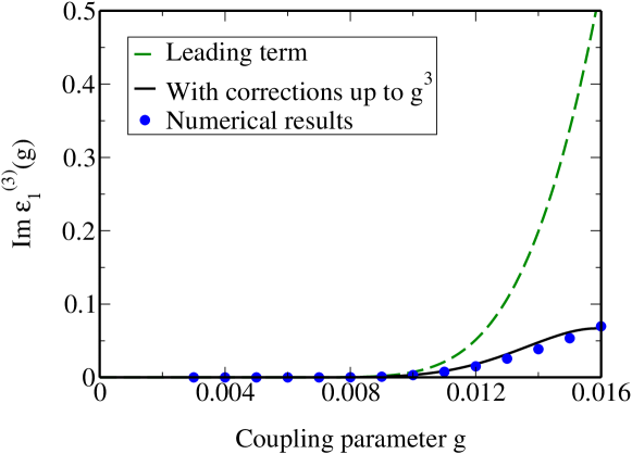
Figure 5.1: Comparison of the analytic results (5.1) and (5.2) with numerical data for the imaginary part ${\rm Im}\,\epsilon_{1}^{(3)}(g)$ of the resonance energy of the first excited state of the cubic potential.

5.2 Numerical Calculations for Weak Coupling

Let us note first of all that all analytic results derived here have been subjected to extensive numerical verification. Here, we would only like to discuss one particular case, the higher-order formula for the subleading corrections to the decay width of the first excited level of the cubic potential, which we recall here from Eq. (4.2),

$${\rm Im}\,\epsilon_{1}^{(3)}(g)=-\frac{8\,{\rm e}^{-2/(15\,g)}}{\sqrt{\pi}\,g^{3/2}}\,\left\{1-\frac{853}{16}\,g+\frac{33349}{512}\,g^{2}-\frac{395368511}{40960}\,g^{3}+{\mathcal{O}}(g^{4})\right\}\,.$$ (5.1)

Our purpose is to compare this result to the numerical values generated exclusively by the leading-order term

$${\rm Im}\,\epsilon_{1,{\rm leading}}^{(3)}(g)=-\frac{8\,{\rm e}^{-2/(15\,g)}}{\sqrt{\pi}\,g^{3/2}}\,.$$ (5.2)

The relative correction of order $g$ as given by the term $-853\,g/16\approx-53\,g$ in Eq. (5.1) is extremely important in reaching satisfactory agreement of the analytic result and numerical data for the imaginary part of the resonance energy ${\rm Im}\,\epsilon_{1}^{(3)}(g)$, even at relatively small coupling parameter $g\leq 0.01$. This is evident from Fig. 5.1, where we compare the leading term of the asymptotics given in Eq. (5.2) as well as the first three correction terms given in Eq. (5.1) to numerical data.

5.3 Numerical Calculations for Large Coupling

As we look at the dispersion relations (2.31b) and (2.31a), we might ask ourselves how far the cut extends: from $g=0$ to $g=\infty$, or possibly up to a finite value of the coupling. Our conjecture here is that the resonances of the unstable oscillators persist for any value of the coupling, however large. Intuition might suggest otherwise. The unstable case is naturally associated with tunneling through the potential barrier. As the coupling increases, the barrier becomes narrower until, in the limit of very large modulus of the coupling, it eventually disappears. One might assume that only a limited number of resonances persist for a large, but finite value of the coupling: namely, only those for which the real part of the energy lies significantly “under the top” of the barrier. Numerical evidence [54] suggests otherwise. Namely, we investigate the strong-coupling expansion for the resonances of odd oscillators. After a scaling transformation $q\to g^{-1/(2(M+2))}\,q$, which leaves the spectrum invariant, the odd Hamiltonian (2.1b) reads

$$h_{{\rm s},M}(g)=g^{1/(M+2)}\,\left(h_{\ell,M}+\frac{1}{2}\,g^{-2/(M+2)}\,q^{2}\right)\,,\qquad h_{\ell,M}=-\frac{1}{2}\,\frac{\partial^{2}}{\partial q^{2}}+q^{M}\,,$$ (5.3)

where $h_{\ell,M}$ does not depend on the coupling $g$. This Hamiltonian now gives the strong-coupling expansion in a natural way: One can regard the term ${\textstyle{\frac{1}{2}}}\,g^{-2/(M+2)}\,q^{2}$ as a perturbation of the term $q^{M}$. Via a complex scaling transformation $q\to q\,{\mathrm{e}}^{{\mathrm{i}}\,\theta_{M}}$, we transform $h_{\ell,M}\to h_{\ell,M}(\theta)$ where

$$h_{\ell,M}(\theta)= \;{\mathrm{e}}^{-2\,{\mathrm{i}}\theta_{M}}\,\left(-\frac{1}{2}\,\frac{\partial^{2}}{\partial q^{2}}+q^{M}\,{\mathrm{e}}^{{\mathrm{i}}\,(M+2)\,\theta_{M}}\right)\,,\qquad\theta_{M}=\frac{\pi}{M+2}\,.$$ (5.4)

A diagonalization of this complex-scaled Hamiltonian in the space of harmonic oscillator eigenfunctions gives us approximations to the resonance energies. The resonance eigenvalues have a well-defined complex argument, and they can be numbered by an index $n=0,1,2,\dots$. They read

$$\epsilon^{(M)}_{\ell,n}=\left|\epsilon^{(M)}_{\ell,n}\right|\,{\mathrm{e}}^{-{\mathrm{i}}\,\pi/(M+2)}\,,$$ (5.5)

where by virtue of (2.31a), we associate the resonance as opposed to the antiresonance with the region infinitesimally above the real axis,

$$\epsilon^{(M)}_{n}(g+{\mathrm{i}}0)=g^{1/(M+2)}\,\left[\epsilon^{(M)}_{\ell,n}+{\mathcal{O}}\left(g^{-2/(M+2)}\right)\right]\,,$$ (5.6)

for $g\to\infty$. These asymptotics suggest that all resonances $n=0,1,2,\dots$ persist for any modulus of the coupling. Specifically, according to Table 2 of [54], we have

$$\epsilon^{(3)}_{\ell,0}=0.762\,851\,775\,{\mathrm{e}}^{-{\mathrm{i}}\,\pi/5}\,,\quad\epsilon^{(3)}_{\ell,1}=2.711\,079\,923\,{\mathrm{e}}^{-{\mathrm{i}}\,\pi/5}\,,\quad\epsilon^{(3)}_{\ell,2}=4.989\,240\,088\,{\mathrm{e}}^{-{\mathrm{i}}\,\pi/5}\,.$$ (5.7)

The above results define the large-coupling coupling asymptotics for the for the first three resonances $\epsilon^{(3)}_{n}(g)\to g^{1/5}\,\epsilon^{(3)}_{\ell,n}$, for $g\to\infty+{\mathrm{i}}0$ (with $n=0,1,2$). We have also obtained corresponding results for higher excited states and conjecture here that all resonances of the cubic oscillator persist for any value of the coupling, however large. The corresponding large-coupling asymptotics for the quantic potential are given by the levels

$$\epsilon^{(5)}_{\ell,0}=0.709\,935\,516\,{\mathrm{e}}^{-{\mathrm{i}}\,\pi/7}\,,\quad\epsilon^{(5)}_{\ell,1}=2.659\,756\,364\,{\mathrm{e}}^{-{\mathrm{i}}\,\pi/7}\,,\quad\epsilon^{(5)}_{\ell,2}=5.458\,235\,423\,{\mathrm{e}}^{-{\mathrm{i}}\,\pi/7}\,.$$ (5.8)

For the even oscillators, the corresponding formulas read as follows. We recall that the resonances appear for negative $g$, and that the resonance as opposed to the antiresonance is attached to the negative $g$ axis for infinitesimal positive imaginary part of the coupling. Under a scaling transformation $q\to(-g)^{-1/(N+2)}\,q$, the Hamiltonian (2.1a) transforms to the following scaled Hamiltonian with the same spectrum,

$$H_{{\rm s},N}(g)=(-g)^{2/(N+2)}\,\left(H_{\ell,N}+\frac{1}{2}\,(-g)^{-4/(N+2)}\,q^{2}\right)\,,\qquad H_{\ell,N}=-\frac{1}{2}\,\frac{\partial^{2}}{\partial q^{2}}-q^{N}\,.$$ (5.9)

As a WKB–approximation to the wave function shows, the appropriate scaling transformation for even $N$ is also of the form $q\to q{\mathrm{e}}^{{\mathrm{i}}\,\theta_{N}}$, but with $H_{\ell,N}(\theta)$ and $\theta_{N}$ given by

$$H_{\ell,N}(\theta)={\mathrm{e}}^{-2{\mathrm{i}}\theta_{N}}\,\left(-\frac{1}{2}\,\frac{\partial^{2}}{\partial q^{2}}-q^{N}\,{\mathrm{e}}^{{\mathrm{i}}\,(N+2)\,\theta_{N}}\right)\,,\qquad\theta_{N}=\frac{2\,\pi}{N+2}\,.$$ (5.10)

The eigenvalues again have a well-defined complex phase,

$$E^{(N)}_{\ell,n}=\left|E^{(N)}_{\ell,n}\right|\,{\mathrm{e}}^{-2\,{\mathrm{i}}\,\pi/(N+2)}\,.$$ (5.11)

The large-coupling asymptotics for the resonances then reads

$$E^{(N)}_{n}(g+{\mathrm{i}}0)=(-g)^{2/(N+2)}\,\left[E^{(N)}_{\ell,n}+{\mathcal{O}}\left(g^{-4/(N+2)}\right)\right]\,,$$ (5.12)

for $g\to-\infty$. A numerical determination of the complex resonance eigenvalues $E^{(N)}_{\ell,n}$ of the non–Hermitian Hamiltonian $H_{\ell,N}(\theta)$ is thus sufficient in order determine the large-coupling asymptotics of the resonance eigenvalues of $H_{{\rm s},N}(g)$, which coincide with the resonance eigenvalues $E^{(N)}_{n}(g+{\mathrm{i}}0)$ of $H_{N}(g)$ attained for $g<0$. For the first three resonances of the quartic potential, we find by numerical calculations,

$$E^{(4)}_{\ell,0}=0.667\,986\,260\,{\mathrm{e}}^{-{\mathrm{i}}\,\pi/3}\,,\quad E^{(4)}_{\ell,1}=2.393\,644\,016\,{\mathrm{e}}^{-{\mathrm{i}}\,\pi/3}\,,\quad E^{(4)}_{\ell,2}=4.696\,795\,386\,{\mathrm{e}}^{-{\mathrm{i}}\,\pi/3}\,.$$ (5.13)

This example, which demonstrates the persistence of the quartic resonances in the strong-coupling limit, concludes our analysis of the complex resonances. Note that the strong-coupling expansions, whose leading terms are indicated in Eqs. (5.6) and (5.12), are in some sense complementary to the weak-coupling expansions (3.6) and (3.6).

Chapter 6 Conclusions

 

Anharmonic oscillators form a very basic model for many physical processes. The anharmonic terms induce coupling among the energy levels of the harmonic oscillator, which can be interpreted as inducing some sort of “higher-harmonic generation” due to the intertwining of an infinite number of harmonic modes in the energy levels of the anharmonic oscillator. At the same time, the anharmonic oscillators represent classically integrable systems. There is no chaos, and therefore, the corresponding quantum systems are amenable to a unified treatment which is based on semiclassical expansions and which is manifest in the generalized quantization conditions (3.5) and (3.5). These quantization conditions allow us to determine the subleading corrections to the decay widths of arbitrary levels of anharmonic oscillators of arbitrary degree.

The formulas for the subleading corrections to the decay width of the resonances, as presented in Eqs. (4.2), (4.3), (4.3), (4.4), (4.5), (4.6) and (4.7) have not yet appeared in the literature to the best of our knowledge. We note, in particular, that the results for the excited states in Eqs. (4.2) and (4.3) are derived on the basis of the generalized quantization conditions; these could not have been obtained by standard field-theoretical investigations which involve a higher-order perturbative expansion about the instanton configurations, as it is the case for the ground-state results (see also Sec. 5.2). All analytic results presented here have been subjected to intensive numerical checks, including those for the sextic anharmonic oscillator where the higher-order corrections are observed to have a rather surprising structure.

Let us now attempt to interpret the results from a broader perspective. In the case of a theory with an “unstable” potential where, classically, the motion of the particle is not confined to a finite spatial region, one typically encounters quantum mechanical resonances with a nonvanishing decay width, when one endows the problem with “outgoing” boundary conditions (and the corresponding antiresonances for the complex conjugated boundary conditions). The complex boundary conditions lead to a non-Hermitian Hamilton operator whose resonance energies are not real. Intuition suggests that there must be way of smoothly changing the coupling constant and the boundary conditions from the “resonance case” to the corresponding complex conjugated antiresonance, so that the resonance eigenvalue “transits” through the real axis. At this point, precisely, at least for the odd anharmonic oscillators, the eigenenergies become real, and the Hamiltonian becomes ${\mathcal{PT}}$-symmetric (see [15]). This is the observation that leads, naturally, to the dispersion relation (2.31a) for odd anharmonic oscillators.

Analogously [39, 20, 6], for even anharmonic oscillators, if one starts from negative coupling, there is a way of changing the complex argument of the coupling parameter so that the boundary conditions for resonances and antiresonances deform smoothly into each other, crossing an entirely real eigenvalue for the energy at positive, and real, coupling $g$, and this corresponds to the relation (2.31b).

In some sense, ${\mathcal{PT}}$-symmetric odd anharmonic oscillators receive an interpretation as the analogy complete analogy of even anharmonic oscillators for positive and real coupling. They provide a bridge between resonances and antiresonances, as exemplified by the dispersion relation (2.31a), over the real axis. They also facilitate the interpretation of theories which allow for the presence of complex resonance and antiresonance energies, by allowing us to interpret these theories as the unstable realizations of a stable, ${\mathcal{PT}}$-symmetric theory, continued into the complex plane.

By a similarity transformation [15, 21, 23, 24], it is possible to map the dynamics induced by a ${\mathcal{PT}}$-symmetric theory onto a Hermitian theory, but the resulting expressions can be very complicated, and even in the case of the relatively simple cubic ${\mathcal{PT}}$-symmetric oscillator, the corresponding Hermitian Hamiltonian obtained by the similarity transformation cannot be written down in closed form and contains operators that mix momenta and coordinates. In that case, the original, ${\mathcal{PT}}$-symmetric theory, namely the ${\mathcal{PT}}$-symmetric cubic oscillator, provides for a much more compact formulation that allows for a workable, and practically feasible formulation in terms of variational principles and corresponding classical trajectories of the dynamical variables, which would be much more difficult to achieve when starting the discussion from the much more involved expressions that occur in a typical case [24] for the equivalent, Hermitian theory. This is one of the reasons why ${\mathcal{PT}}$-symmetric theories have received some attention in the physics community in recent years.

Although a high degree of unification can been achieved for odd versus even anharmonic oscillators using concepts from ${\mathcal{PT}}$-symmetry and generalized quantization conditions, let us finally, that there is some room left for future investigations. E.g., one might well ask what the quantization conditions (2.31a) and (2.31b) should look like for arbitrary complex argument of the coupling $g$. Our conjectures as presented in Eqs. (3.5), (3.5) and (3.71) are relevant only for either positive or negative, or purely imaginary coupling parameter. These parameter ranges represent the physically most important scenarios by far, but we would like to point out that the interpolation required to describe an arbitrary complex argument of the coupling parameter remains an open problem.

Finally, in view of the phenomenological significance of anharmonic oscillators, we believe that the numerically large correction terms in the higher-order formulas for the decay widths, as obtained, e.g., in Eqs. (4.2) and (4.3), might find interesting applications in the various branches of the theory of finite quantum systems.

Bibliography

- [1] J. Zinn-Justin, U. D. Jentschura, Multi–Instantons and Exact Results I: Conjectures, WKB Expansions, and Instanton Interactions, Ann. Phys. (N.Y.) 313 (2004) 197–267.
- [2] J. Zinn-Justin, U. D. Jentschura, Multi–Instantons and Exact Results II: Specific Cases, Higher-Order Effects, and Numerical Calculations, Ann. Phys. (N.Y.) 313 (2004) 269–325.
- [3] U. D. Jentschura, A. Surzhykov, J. Zinn-Justin, Unified Treatment of Even and Odd Anharmonic Oscillators of Arbitrary Degree, Phys. Rev. Lett. 102 (2009) 011601.
- [4] S. Graffi, V. Grecchi, B. Simon, Borel summability: application to the anharmonic oscillator, Phys. Lett. B 32 (1970) 631–634.
- [5] E. Balslev, J. C. Combes, Spectral properties of many-body Schrödinger operators with dilation-analytic interactions, Commun. Math. Phys. 22 (1971) 280–294.
- [6] C. M. Bender, T. T. Wu, Anharmonic oscillator. II. A study in perturbation theory in large order, Phys. Rev. D 7 (1973) 1620–1636.
- [7] A. Voros, The return of the quartic oscillator. The complex WKB method, Ann. Inst. Henri Poincaré A 39 (1983) 211–338.
- [8] E. J. Weniger, A convergent renormalized strong coupling perturbation expansion for the ground state energy of the quartic, sextic, and octic anharmonic oscillator, Ann. Phys. (N.Y.) 246 (1996) 133–165.
- [9] E. J. Weniger, Construction of the strong coupling expansion for the ground state energy of the quartic, sextic and octic anharmonic oscillator via a renormalized strong coupling expansion, Phys. Rev. Lett. 77 (1996) 2859–2862.
- [10] I. W. Herbst, B. Simon, Some remarkable examples in eigenvalue perturbation theory, Phys. Lett. B 78 (1978) 304–306.
- [11] E. Caliceti, V. Grecchi, M. Maioli, Double wells: Perturbation series summable to eigenvalues and directly computable approximants, Commun. Math. Phys. 113 (1988) 625–648.
- [12] E. Caliceti, V. Grecchi, M. Maioli, Double wells: Nevanlinna analyticity, distributional Borel sum and asymptotics, Commun. Math. Phys. 176 (1996) 1–22.
- [13] U. D. Jentschura, J. Zinn-Justin, Instanton Effects in Quantum Mechanics and Resurgent Expansions, Phys. Lett. B 596 (2004) 138–144.
- [14] C. M. Bender, G. V. Dunne, Large-order perturbation theory for a non-Hermitian -symmetric Hamiltonian, J. Math. Phys. 40 (1999) 4616–4621.
- [15] C. M. Bender, S. Boettcher, Real Spectra in Non-Hermitian Hamiltonians Having -Symmetry, Phys. Rev. Lett. 80 (1998) 5243–5246.
- [16] C. M. Bender, S. Boettcher, P. N. Meisinger, -symmetric quantum mechanics, J. Math. Phys. 40 (1999) 2201–2229.
- [17] C. M. Bender, E. J. Weniger, Numerical evidence that the perturbation expansion for a non-Hermitian -symmetric Hamiltonian is Stieltjes, J. Math. Phys. 42 (2001) 2167–2183.
- [18] C. M. Bender, G. V. Dunne, P. N. Meisinger, M. Simsek, Quantum complex Hénon–Heiles potentials, Phys. Lett. A 281 (2001) 311–316.
- [19] C. M. Bender, D. C. Brody, H. F. Jones, Complex Extension of Quantum Mechanics, Phys. Rev. Lett. 89 (2002) 270401.
- [20] C. M. Bender, T. T. Wu, Large-order behavior of perturbation theory, Phys. Rev. Lett. 27 (1971) 461–465.
- [21] A. Mostafazadeh, Pseudo–hermiticity versus -symmetry: The necessary condition for the reality of the spectrum of a non-Hermitian hamiltonian, J. Math. Phys. 43 (2002) 205–214.
- [22] A. Mostafazadeh, Pseudo-hermiticity versus -symmetry II: A complete characterization of non-Hermitian hamiltonians with a real spectrum, J. Math. Phys. 43 (2002) 2814–2816.
- [23] A. Mostafazadeh, Pseudo-hermiticity versus -symmetry III: Equivalence of pseudo-hermiticity and the presence of antilinear symmetries, J. Math. Phys. 43 (2002) 3944–3951.
- [24] A. Mostafazadeh, -symmetric cubic anharmonic oscillator as a physical model, J. Phys. A 38 (2005) 6657–6569.
- [25] A. Matzkin, Non-hermitian quantum mechanics: the case of bound state scattering theory, J. Phys. A 39 (2006) 10859–10870.
- [26] M. Znojil, Discrete -symmetric models of scattering, J. Phys. A 41 (2008) 292002.
- [27] A. Ruschhaupt, F. Delgado, J. G. Muga, Physical realization of -symmetric potential scattering in a planar slab waveguide, J. Phys. A 38 (2005) L171–L176.
- [28] A. Mostafazadeh, F. Loran, Propagation of electromagnetic waves in linear media and pseudo-Hermiticity, Europhys. Lett. 81 (2008) 10007.
- [29] Z. H. Musslimani, K. G. Makris, R. El-Ganainy, D. N. Christodoulides, Optical solitons in -symmetric potentials, Phys. Rev. Lett. 100 (2008) 030402.
- [30] D. Krejcirik, M. Tater, Non-hermitian spectral effects in a -symmetric waveguide, J. Phys. A 41 (2008) 244013.
- [31] R. N. Deb, N. Bayak, B. Dutta-Roy, Squeezed atomic states, pseudo-Hermitian operators and Wigner D-matrices, Eur. Phys. J. D 33 (2005) 149–155.
- [32] A. A. Andrianov, F. Cannata, P. Giacconi, A. Y. Kamenshchik, D. Regoli, Two-field cosmological models and large-scale cosmic magnetic fields, J. Cosmology Astroparticle Phys. 10 (2008) 019.
- [33] C. M. Bender, S. F. Brandt, J. H. Chen, Q. Wang, Ghost busting: -symmetric interpretation of the Lee model, Phys. Rev. D 71 (2008) 025014.
- [34] C. M. Bender, P. D. Mannheim, No-ghost theorem for the fourth-order derivative Pais-Uhlenbeck oscillator model, Phys. Rev. Lett. 100 (2008) 110402.
- [35] J. Zinn-Justin, Intégrale de chemin en mécanique quantique: Introduction, CNRS Éditions, Paris, 2003.
- [36] J. C. Le Guillou, J. Zinn-Justin, Critical exponents from field theory, Phys. Rev. B 21 (1980) 3976–3998.
- [37] J. Zinn-Justin, Quantum Field Theory and Critical Phenomena, 3rd Edition, Clarendon Press, Oxford, 1996.
- [38] E. Brézin, G. Parisi, J. Zinn-Justin, Perturbation theory at large order. I. The interaction, Phys. Rev. D 15 (1977) 1544–1557.
- [39] J. Loeffel, A. Martin, B. Simon, A. S. Wightman, Padé approximants and the anharmonic oscillator, Phys. Lett. B 30 (1969) 656–658.
- [40] L. D. Landau, E. M. Lifshitz, Quantum Mechanics, Pergamon Press, Oxford, UK, 1958.
- [41] C. M. Bender, S. A. Orszag, Advanced Mathematical Methods for Scientists and Engineers, McGraw-Hill, New York, NY, 1978.
- [42] R. P. Feynman, Space–Time Approach to Quantum Electrodynamics, Phys. Rev. 76 (1949) 769–789.
- [43] K. Pachucki, Higher-Order Binding Corrections to the Lamb Shift, Ann. Phys. (N.Y.) 226 (1993) 1–87.
- [44] U. Jentschura, K. Pachucki, Higher-order binding corrections to the Lamb shift of states, Phys. Rev. A 54 (1996) 1853–1861.
- [45] V. Franceschini, V. Grecchi, H. J. Silverstone, Complex energies from real perturbation series for the LoSurdo-Stark effect in Hydrogen by Borel-Padé approximants, Phys. Rev. A 32 (1985) 1338–1340.
- [46] U. D. Jentschura, Resummation of the divergent perturbation series for a hydrogen atom in an electric field, Phys. Rev. A 64 (2001) 013403.
- [47] U. D. Jentschura, J. Zinn-Justin, Higher-order corrections to instantons, J. Phys. A 34 (2001) L253–L258.
- [48] G. Alvarez, Coupling-constant behavior of the resonances of the cubic anharmonic oscillator, Phys. Rev. A 37 (1988) 4079–4083.
- [49] G. Baym, Inconsistency in cubic boson–boson interactions, Phys. Rev. 117 (1960) 886–888.
- [50] A. J. McKane, Vacuum instability in scalar field theories, Nucl. Phys. B 152 (1979) 166–188.
- [51] J. Feinberg, Y. Peleg, Self-adjoint Wheeler–DeWitt operators, the problem of time, and the wave function of the Universe, Phys. Rev. D 52 (1995) 1988–2000.
- [52] J. P. Killingbeck, A. Grosjean, G. Jolicard, Complex variable HVPT, J. Phys. A 37 (2004) 7971–7976.
- [53] J. P. Killingbeck, A. Grosjean, G. Jolicard, Complex HVPT and hyperasymptotics, J. Phys. A 39 (2006) L547–L550.
- [54] U. D. Jentschura, A. Surzhykov, M. Lubasch, J. Zinn-Justin, Structure, time propagation and dissipative terms for resonances, J. Phys. A 41 (2008) 095302.
- [55] A. V. Sergeev, D. Z. Goodson, Summation of asymptotic expansions of multiple-valued functions using algebraic approximants: Application to anharmonic oscillators, J. Phys. A 31 (1998) 4301–4317.
- [56] F. M. Fernández, R. Guardiola, J. Ros, M. Znojil, Strong-coupling expansions for the -symmetric oscillators , J. Phys. A 31 (2005) 10105–10112.
- [57] P. Dorey, C. Dunning, R. Tateo, Supersymmetry and the spontaneous breakdown of -symmetry, J. Phys. A 34 (2002) L391–L400.
- [58] P. Dorey, C. Dunning, R. Tateo, Spectral equivalences, Bethe ansatz equations, and reality properties in -symmetric quantum mechanics, J. Phys. A 34 (2002) 5679–5704.
- [59] E. Caliceti, Distributional Borel summability of odd anharmonic oscillators, J. Phys. A 33 (2000) 3753–3770.
- [60] E. Caliceti, V. Grecchi, M. Maioli, The Distributional Borel Summability and the Large Coupling Lattice Fields, Commun. Math. Phys. 104 (1986) 163–174.
- [61] E. Caliceti, M. Meyer-Hermann, P. Ribeca, A. Surzhykov, U. D. Jentschura, From useful algorithms for slowly convergent series to physical predictions based on divergent perturbative expansions, Phys. Rep. 446 (2007) 1–96.