Moments of Spin Structure Functions: Sum Rules and Polarizabilities

Abstract

Nucleon structure study is one of the most important research areas in modern physics and has challenged us for decades. Spin has played an essential role and often brought surprises and puzzles to the investigation of the nucleon structure and the strong interaction. New experimental data on nucleon spin structure at low to intermediate momentum transfers combined with existing high momentum transfer data offer a comprehensive picture in the strong region of the interaction and of the transition region from the strong to the asymptotic-free region. Insight for some aspects of the theory for the strong interaction, Quantum Chromodynamics (QCD), is gained by exploring lower moments of spin structure functions and their corresponding sum rules (i.e. the Bjorken, Burkhardt-Cottingham, Gerasimov-Drell-Hearn (GDH), and the generalized GDH). These moments are expressed in terms of an operator-product expansion using quark and gluon degrees of freedom at moderately large momentum transfers. The higher-twist contributions have been examined through the evolution of these moments as the momentum transfer varies from higher to lower values. Furthermore, QCD-inspired low-energy effective theories, which explicitly include chiral symmetry breaking, are tested at low momentum transfers. The validity of these theories is further examined as the momentum transfer increases to moderate values. It is found that chiral perturbation theory calculations agree reasonably well with the first moment of the spin structure function $g_{1}$ at low momentum transfer of 0.05 - 0.1 GeV² but fail to reproduce some of the higher moments, noticeably, the neutron data in the case of the generalized polarizability $\delta_{LT}$. The Burkhardt-Cottingham sum rule has been verified with good accuracy in a wide range of $Q^{2}$ assuming that no singular behavior of the structure functions is present at very high excitation energies.

1 Introduction

The nucleons (proton and neutron), the basic building blocks of nuclear matter, account for more than $99.9\%$ of the mass of the visible matter in the universe. Understanding the nucleon structure is one of the most important issues in modern physics and has challenged us for decades. The internal structure of the nucleon presents a wealth of fundamental questions, that have a deep impact on our understanding of Nature and the universe we live in.

The strong interaction, that is mostly responsible for the structure of the nucleon, poses a special challenge to us due to the strong and non-linear nature of the force. Quantum Chromodynamics (QCD) is the accepted theory for the strong interaction. Quarks and gluons are the fundamental particles and force mediators, while nucleons and mesons (pions, kaons, etc.), collectively called hadrons, are composite particles and effective force mediators. QCD has been well tested at high energy (asymptotic-free) when the interaction is relatively weak due to the running of strong coupling constant. However, at low energy (scale of the size of a hadron), the strong force becomes truly strong, leading to chiral symmetry breaking and the confinement of the quarks and gluons inside the hadron where none can escape to become free particles. In the strong region of QCD, the usual calculation technique of perturbative expansion fails, and QCD can not be easily solved. Effective field theories, such as chiral perturbation theory [1], are often used. Recently, great progress has been made in the advancement of lattice QCD [2], which has begun to provide some calculations of QCD in the strong region. Another approach [3] is to stay with the continuous field theory by using the Schwinger-Dyson equations. Newly developed anti-de Sitter/conformal field theory (AdS/CFT) [4] might provide another useful tool to study strong QCD.

In addition to the truly strong region, understanding the transition from weak (perturbative) to strong (non-perturbative) region is also very important. One approach is to start from high energy where the quarks and gluons (collectively called partons) are asymptotically free. With the help of the Operator Product Expansion (OPE) [5, 6, 7], one can systematically expand to a twist series, where the leading twist term gives the parton distributions and the higher-twist terms characterize the quark-gluon and quark-quark correlations. Lattice QCD can also provide useful calculations. Constituent-quark models are also often used to provide intuitive pictures in this region.

Experimentally, deep-inelastic lepton scattering (DIS) together with other processes, such as Drell-Yan, direct photon and heavy quark productions, have been powerful tools to study nucleon structure. The unpolarized structure functions extracted from the last five decades, covering five-order of magnitudes in both $Q^{2}-$ and $x-$ranges, are the most extensive set of precision data in nucleon structure study. The longitudinally polarized structure functions extracted from the last three decades have reached reasonable precision, covering two to three-order of magnitudes in $Q^{2}-$ and $x-$ ranges. Transversely polarized measurements have been the recent focus, but are still scarce. The lower moments of the structure functions provide the most direct tests and comparisons with theoretical calculations through sum rules.

In the study of nucleon structure, spin has played an essential role and often brought big surprises. Spin was first introduced as an internal property of a particle, related to the magnetic moment, to explain the famous Stern-Gerlach results [8] that the silver atoms split into two beams after passing through an inhomogeneous magnetic field. The discovery of the anomalous magnetic moment of the proton [9] was the first big spin surprise. This discovery was the beginning of the (indirect) study of nucleon structure, since the anomalous magnetic moment was one piece of evidence for the internal structure of the nucleon. Later on, it was related to the integration of the excitation spectrum of nucleon spin structure by the sum rule of Gerasimov, Drell and Hearn (GDH) [10, 11]. The direct study of nucleon structure started decades later when Hofstadter [12] used elastic electron scattering to directly measure the form factors of the proton.

In the last thirty years, the spin structure of the nucleon has led to very productive experimental and theoretical activity with exciting results and new challenges[13]. This investigation has included a variety of aspects such as testing QCD in its perturbative region via spin sum rules (like the Bjorken sum rule[14]) and understanding how the spin of the nucleon is built from the intrinsic degrees of freedom of the theory: quarks and gluons. Recently, results from a new generation of experiments performed at Jefferson Lab seeking to probe the theory in its non-perturbative and transition regions have reached a mature state. The low momentum-transfer results offer insight in a region characterized by the collective behavior of the nucleon constituents and their interactions. In this region, it has been more economical to describe the nucleon using effective degrees of freedom like mesons and constituent quarks rather than current quarks and gluons. Furthermore, distinct features seen in the nucleon response to the electromagnetic probe, depending on the resolution of the probe, point clearly to different regions of description, i.e. a scaling region where quark-gluon correlations are suppressed versus a coherent region where long-range interactions give rise to the static properties of the nucleon.

In this review we describe an investigation [15]^-[32] of the spin structure of the nucleon through measurements of the helicity-dependent photoabsorption cross sections or asymmetries by using virtual photons covering a wide resolution spectrum. These observables are used to extract the spin structure functions $g_{1}$ and $g_{2}$ and evaluate their moments. These moments are key ingredients to test QCD sum rules and unravel some aspects of the quark-gluon structure of the nucleon.

2 Formalism

Leptons do not involve the strong interaction directly. With the electromagnetic interaction well-understood, lepton beams have been a very powerful precision probe to study nucleon structure. Consider deep-inelastic scattering of polarized leptons on polarized nucleons. We denote by $m$ the lepton mass, $k~{}(k^{\prime}$) the initial (final) lepton four-momentum and $s~{}(s^{\prime})$ its covariant spin four-vector, such that $s\cdot k$ = 0 $(s^{\prime}\cdot k^{\prime}=0)$ and $s\cdot s=-1$ $(s^{\prime}\cdot s^{\prime}=-1)$; the nucleon mass is $M$ and the nucleon four-momentum and spin four-vector are, respectively, $P$ and $S$. Assuming, as is usually done, one-photon exchange (see Fig. 1), the differential cross section for detecting the final polarized lepton within the solid angle $d\Omega$ and the final energy range $(E^{\prime},~{}E^{\prime}+dE^{\prime})$ in the laboratory frame $P=(M,\bm{0}),~{}k=(E,\bm{k}),~{}k^{\prime}=(E^{\prime},\bm{k}^{\prime})$, can be written as

$$\frac{d^{2}\sigma}{d\Omega dE^{\prime}}=\frac{\alpha^{2}}{2Mq^{4}}\frac{E^{\prime}}{E}L_{\mu\nu}W^{\mu\nu},$$ (1)

where $q=k-k^{\prime}$ and $\alpha$ is the fine structure constant.

file=DIS-Feynman,scale=0.7

Figure 1: Feynman diagram for deep-inelastic lepton-hadron scattering

The leptonic tensor $L_{\mu\nu}$ is given by

$$L_{\mu\nu}(k,s;k^{\prime})=\sum_{s^{\prime}}\,[\bar{u}(k^{\prime},s^{\prime})~{}\gamma_{\mu}~{}u(k,s)]^{\ast}~{}[\bar{u}(k^{\prime},s^{\prime})~{}\gamma_{\nu}~{}u(k,s)]$$ (2)

and can be split into symmetric $(S)$ and antisymmetric $(A)$ parts under $\mu$ and $\nu$ interchange:

$$L_{\mu\nu}(k,s;k^{\prime})=2\{L^{(S)}_{\mu\nu}~{}(k;k^{\prime})+iL^{(A)}_{\mu\nu}~{}(k,s;k^{\prime})\}$$ (3)

where $u(k,s)$ and $\bar{u}(k^{\prime},s^{\prime})$ are electron spinors, and

$$L^{(S)}_{\mu\nu}~{}(k;k^{\prime}) = k_{\mu}k^{\prime}_{\nu}+k^{\prime}_{\mu}k_{\nu}-g_{\mu\nu}~{}(k\cdot k^{\prime}-m^{2})$$ (4)

$$L^{(A)}_{\mu\nu}~{}(k,s;k^{\prime}) = m~{}\varepsilon_{\mu\nu\alpha\beta}~{}s^{\alpha}~{}q^{\beta}.$$ (5)

The unknown hadronic tensor $W_{\mu\nu}$ describes the interaction between the virtual photon and the nucleon and depends upon four scalar structure functions: the unpolarized functions $F_{1,2}$ and the spin-dependent functions $g_{1,2}$ (ignoring parity-violating interactions). These functions contain information on the internal structure of the nucleon. They can be experimentally measured and then be studied in theoretical models, such as the QCD-parton model. The functions can only depend on the scalars $q^{2}$ and $q\cdot P$. Usually people work with

$$Q^{2}\equiv-q^{2}\quad\textrm{and}\quad x\equiv Q^{2}/2q\cdot P=Q^{2}/2M\nu$$ (6)

where $\nu=E-E^{\prime}$ is the energy of the virtual photon in the Lab frame. The variable $x$, known as “$x$-Bjorken”, is the fraction of momentum carried by the struck quark in the simple parton model. We also refer to the invariant mass of the (unobserved) final state, $W=(P+q)^{2}=M^{2}+2M\nu-Q^{2}$.

Analogous to Eq. (3) one has

$$W_{\mu\nu}(q;P,S)=W^{(S)}_{\mu\nu}(q;P)+i~{}W_{\mu\nu}^{(A)}(q;P,S).$$ (7)

The symmetric part, relevant to unpolarized DIS, is given by

$$W^{(S)}_{\mu\nu}(q;P) = 2\left[\frac{q_{\mu}q_{\nu}}{q^{2}}-g_{\mu\nu}\right]\,F_{1}(x,Q^{2})$$

$$+\frac{2}{M\nu}\left[P_{\mu}-\frac{P\centerdot q}{q^{2}}q_{\mu}\right]\left[P_{\nu}-\frac{P\centerdot q}{q^{2}}q_{\nu}\right]\,F_{2}(x,Q^{2}).$$

The antisymmetric part, relevant for polarized DIS, can be written as

$$W^{(A)}_{\mu\nu}(q;P,s)=2~{}\varepsilon_{\mu\nu\alpha\beta}~{}q^{\alpha}\Biggl{\{}M^{2}S^{\beta}G_{1}(\nu,Q^{2})+\left[M\nu S^{\beta}-(S\cdot q)\,P^{\beta}\right]G_{2}(\nu,Q^{2})\Biggl{\}}$$ (9)

or, in terms of the scaling functions $g_{1,2}$

$$g_{1}(x,Q^{2})=M^{2}\nu G_{1}(\nu,Q^{2}),\qquad g_{2}(x,Q^{2})=M\nu^{2}G_{2}(\nu,Q^{2}),$$ (10)

$$W^{(A)}_{\mu\nu}(q;P,s)=\frac{2M}{P\cdot q}~{}\varepsilon_{\mu\nu\alpha\beta}~{}q^{\alpha}\Biggl{\{}S^{\beta}g_{1}(x,Q^{2})+\left[S^{\beta}-\frac{(S\cdot q)\,P^{\beta}}{(P\cdot q)}\right]g_{2}(x,Q^{2})\Biggl{\}}\,.$$ (11)

Note that these expressions are electromagnetically gauge-invariant:

$$q^{\mu}W_{\mu\nu}=0.$$ (12)

In the Bjorken limit, or deep-inelastic regime,

$$Q^{2}\to\infty\quad,\quad\nu\to\infty\quad,\quad x\,\,\rm{fixed},$$ (13)

the structure functions $F_{1,2}$ and $g_{1,2}$ are known to approximately scale, i.e., vary very slowly with $Q^{2}$ at fixed $x$ – in the simple parton model they scale exactly; in QCD their $Q^{2}$-evolution can be calculated perturbatively.

The differential cross section for unpolarized leptons scattering off an unpolarized target can be written as

$$\frac{d^{2}\sigma}{d\Omega~{}dE^{\prime}}(k,s,P,-S;k^{\prime})=\frac{\alpha^{2}}{2Mq^{4}}~{}\frac{E^{\prime}}{E}~{}2L_{\mu\nu}^{(S)}~{}W^{\mu\nu(S)}.$$ (14)

While differences of cross sections with opposite target spins are given by

$$\left[\frac{d^{2}\sigma}{d\Omega~{}dE^{\prime}}(k,s,P,-S;k^{\prime})-\frac{d^{2}\sigma}{d\Omega~{}dE^{\prime}}~{}(k,s,P,S;k^{\prime})\right]=\frac{\alpha^{2}}{2Mq^{4}}~{}\frac{E^{\prime}}{E}~{}4L_{\mu\nu}^{(A)}~{}W^{\mu\nu(A)}.$$ (15)

After some algebra [36], one obtains from Eqs. (4,5,2,11,14,15) expressions for the unpolarized cross section and polarized cross-section differences (note that the lepton-mass terms are neglected):

• The unpolarized cross section is given by

  $$\frac{d^{2}\sigma_{unpold}}{d\Omega~{}dE^{\prime}}=\Bigl{(}\frac{d\sigma}{d\Omega}\Bigr{)}_{Mott}\Bigl{[}\frac{2}{M}F_{1}(x,Q^{2})\tan^{2}\frac{2}{\theta}+\frac{1}{\nu}F_{2}(x,Q^{2})\Bigr{]}$$ (16)

  where $\theta$ is the scattering angle in the laboratory frame and the Mott cross section is given by

  $$\Bigl{(}\frac{d\sigma}{d\Omega}\Bigr{)}_{Mott}=\frac{\alpha^{2}\cos^{2}\frac{\theta}{2}}{4E^{2}\sin^{4}\frac{\theta}{2}}.$$ (17)

• For the lepton and target nucleon polarized longitudinally, i.e. along or opposite to the direction of the lepton beam, the cross-section difference under reversal of the nucleon’s spin direction (indicated by the double arrow) is given by

  $$\frac{d^{2}\sigma^{\begin{array}[]{c}\to\vspace*{-0.2cm}\\ \Leftarrow\end{array}}}{d\Omega~{}dE^{\prime}}-\frac{d^{2}\sigma^{\begin{array}[]{c}\to\vspace*{-0.2cm}\\ \Rightarrow\end{array}}}{d\Omega~{}dE^{\prime}}=-\frac{4\alpha^{2}E^{\prime}}{\nu EQ^{2}}\Biggl{[}(E+E^{\prime}\cos\theta)~{}g_{1}(x,Q^{2})-2Mxg_{2}(x,Q^{2})\Biggl{]}~{}.$$ (18)

• For nucleons polarized transversely in the scattering plane, one finds

  $$\frac{d^{2}\sigma^{\to\Uparrow}}{d\Omega~{}dE^{\prime}}-\frac{d^{2}\sigma^{\to\Downarrow}}{d\Omega~{}dE^{\prime}}=-\frac{4\alpha^{2}{E^{\prime}}^{2}}{\nu EQ^{2}}~{}\left[g_{1}(x,Q^{2})+\frac{2ME}{\nu}g_{2}(x,Q^{2})\right]\,.$$ (19)

These two independent observables allow measurement of both $g_{1}$ and $g_{2}$ (as has been done at SLAC and in Jefferson Lab’s Halls A and C), but the transverse cross section difference is generally smaller because of kinematic factors and therefore more difficult to measure. Only in the past decade has it been possible to gather precise information on $g_{2}$, which indeed turns out to be usually smaller than $g_{1}$ in the deep-inelastic region.

Experimental results are often presented in the form of asymmetries, which are ratios of the cross-section differences to the unpolarized cross section.

For a longitudinally polarized target, the measured asymmetry is

$$A_{\|}\equiv\frac{d\sigma^{\begin{array}[]{c}\to\vspace*{-0.2cm}\\ \Leftarrow\end{array}}-d\sigma^{\begin{array}[]{c}\to\vspace*{-0.2cm}\\ \Rightarrow\end{array}}}{2\,d\sigma_{unpold}}$$ (20)

and for a transversely polarized target

$$A_{\perp}\equiv\frac{d\sigma^{\to\Uparrow}-d\sigma^{\to\Downarrow}}{2d\sigma_{unpold}}.$$ (21)

It is customary to introduce the (virtual) photon-nucleon asymmetries $A_{1,2}$:

$$A_{1}=\frac{\sigma_{TT}}{\sigma_{T}}=\frac{g_{1}-\gamma^{2}g_{2}}{F_{1}}$$ (22)

and

$$A_{2}=\frac{\sigma_{LT}}{\sigma_{T}}=\gamma\,\big{[}\frac{g_{1}+g_{2}}{F_{1}}\big{]},$$ (23)

where

$$\gamma=\frac{2Mx}{Q}=\frac{Q}{\nu}~{},$$ (24)

and $\sigma_{T}$, $\sigma_{TT}$ and $\sigma_{LT}$ are the virtual photon cross sections (see below for the definitions of virtual photon cross sections).

From Eqs. (16,18,19), it follows that

$$A_{\|}=D\,(A_{1}+\eta A_{2})$$ (25)

and

$$A_{\perp}=d(A_{2}-\xi A_{1})$$ (26)

where

$$D=\frac{y[(1+\gamma^{2}y/2)(2-y)-2y^{2}m^{2}/Q^{2}]}{y^{2}(1-2m^{2}/Q^{2})(1+\gamma^{2})+2(1+R)(1-y-\gamma^{2}y^{2}/4)}$$ (27)

$$d=\left[\frac{[1+\gamma^{2}y/2(1+2m^{2}y/Q^{2})]\sqrt{1-y-\gamma^{2}y^{2}/4}}{(1-y/2)(1+\gamma^{2}y/2)-y^{2}m^{2}/Q^{2}}\right]\,D$$ (28)

$$\eta=\gamma\,\frac{[1-y-y^{2}(\gamma^{2}/4+m^{2}/Q^{2})]}{(1-y/2)(1+\gamma^{2}y/2)-y^{2}m^{2}/Q^{2}}$$ (29)

$$\xi=\gamma\frac{1-y/2-y^{2}m^{2}/Q^{2}}{1+\gamma^{2}y/2(1+2m^{2}y/Q^{2})},$$ (30)

where

$$y=\frac{\nu}{E},$$ (31)

and

$$R=(1+\gamma^{2})\left(\frac{F_{2}}{2xF_{1}}\right)-1=\frac{\sigma_{L}}{\sigma_{T}}$$ (32)

is the ratio of the longitudinal and transverse virtual photon cross sections.

There exists a restrictive bound on $A_{2}$ [37, 38]:

$$|A_{2}|\leq\sqrt{R\,(1+A_{1})/2}.$$ (33)

In the virtual photon notation, the inclusive inelastic cross section can be written in terms of a virtual photon flux factor and four partial cross sections[39]

$$\frac{d^{2}\sigma}{d\Omega~{}dE^{\prime}}=\Gamma_{V}\sigma(\nu,Q^{2}),$$ (34)

$$\sigma=\sigma_{T}+\epsilon\sigma_{L}-hP_{x}\sqrt{2\epsilon(1-\epsilon)}\sigma_{LT}-hP_{z}\sqrt{1-\epsilon^{2}}\sigma_{TT},$$ (35)

with the photon polarization

$$\epsilon=\frac{1}{1+2(1+\nu^{2}/Q^{2})\tan^{2}(\theta/2)}~{},$$ (36)

and the flux factor

$$\Gamma_{V}=\frac{\alpha E^{\prime}K}{2\pi^{2}EQ^{2}(1-\epsilon)}~{},$$ (37)

where $K$ is the “equivalent photon energy” and here we will use the definition according to Hand[40]

$$K=\nu(1-x)=\frac{W^{2}-M^{2}}{2M}~{}.$$ (38)

$h=\pm 1$ refers to the two helicity states of the (relativistic) lepton. $P_{z}$ is the target polarization along the direction of the virtual photon and $P_{x}$, perpendicular to that direction in the scattering plane of the electron.

The partial cross sections are related to the structure functions as follows:

$$\sigma_{T}=\sigma_{1/2}+\sigma_{3/2}=\frac{4\pi^{2}\alpha}{MK}F_{1}~{},$$ (39)

$$\sigma_{L}=\frac{4\pi^{2}\alpha}{MK}\bigl{[}\frac{1+\gamma^{2}}{\gamma^{2}\nu}F_{2}-\frac{1}{M}F_{1}\bigr{]}~{},$$ (40)

$$\sigma_{TT}=\sigma_{1/2}-\sigma_{3/2}=\frac{4\pi^{2}\alpha}{MK}(g_{1}-\gamma^{2}g_{2})~{},$$ (41)

$$\sigma_{LT}=\frac{4\pi^{2}\alpha}{MK}\gamma(g_{1}+g_{2})~{},$$ (42)

where $\sigma_{1/2}$ and $\sigma_{3/2}$ are the helicity cross sections with 1/2 and 3/2 referring to the total helicity of the (virtual) photon-nucleon system.

Note that in the above we have kept terms of order $M^{2}/Q^{2}$ and smaller. They are sometimes necessary in order to extract the correct experimental values of the structure functions from the measured asymmetries. However, the QCD analysis of the structure functions is often carried out at leading twist only, ignoring higher-twist terms, i.e., higher order in $M^{2}/Q^{2}$. This is clearly inconsistent in cases where the above terms could be important, for example Jefferson Lab experiments.

3 Sum rules and Moments

Sum rules involving the spin structure of the nucleon offer an important opportunity to study QCD. In recent years the Bjorken sum rule at large $Q^{2}$ and the GDH sum rule at $Q^{2}=0$ have attracted large experimental[33, 34, 35] and theoretical[43] efforts that have provided us with rich information. This first type of sum rules relates the moments of the spin structure functions (or, equivalently, the spin-dependent virtual photon cross sections) to the nucleon’s static properties. The second type of sum rules, such as the generalized GDH sum rule[44, 45] or the polarizability sum rules[46, 47], relate the moments of the spin structure functions to real or virtual Compton amplitudes, which can be calculated theoretically. Both types of sum rules are based on “unsubtracted” dispersion relations and the optical theorem[48]. The first type of sum rules uses one more general assumption such as a low-energy theorem[49] for the GDH sum rule and the Operator Production Expansion (OPE)[50] for the Bjorken sum rule to relate the Compton amplitude to a static property.

The formulation below follows closely Refs. [46, 47]. Consider the forward doubly-virtual Compton scattering (VVCS) of a virtual photon with space-like four-momentum q, i.e., $q^{2}=\nu^{2}-{\vec{q}}^{2}=-Q^{2}<0$. The absorption of a virtual photon on a nucleon is related to inclusive electron scattering. As discussed in the previous section, the inclusive cross section contains four partial cross sections (or structure functions): $\sigma_{T}$, $\sigma_{L}$, $\sigma_{TT}$, $\sigma_{LT}$, (or $F_{1}$, $F_{2}$, $g_{1}$, $g_{2}$). In this review, we will concentrate on the spin-dependent functions, $\sigma_{TT}$, $\sigma_{LT}$ (or $g_{1}$, $g_{2}$). In the following discussion, we will start with the general situation, i.e., sum rules valid for all $Q^{2}$, then discuss the two limiting cases at low $Q^{2}$ and at high $Q^{2}$.

Considering the spin-flip VVCS amplitude $g_{TT}$ and assuming it has an appropriate convergence behavior at high energy, an unsubtracted dispersion relation leads to the following equation for $g_{TT}$:

$${\rm Re}[{g}_{TT}(\nu,Q^{2})-g^{pole}_{TT}(\nu,Q^{2})]=(\frac{\nu}{2\pi^{2}}){\cal P}\int^{\infty}_{\nu_{0}}\frac{K(\nu^{\prime},Q^{2})\sigma_{TT}(\nu^{\prime},Q^{2})}{\nu^{\prime 2}-\nu^{2}}d\nu^{\prime},$$ (43)

where $g_{TT}^{pole}$ is the nucleon pole (elastic) contribution, ${\cal P}$ denotes the principal value integral. The lower limit of the integration $\nu_{0}$ is the pion-production threshold on the nucleon. A low-energy expansion gives:

$${\rm Re}[g_{TT}(\nu,Q^{2})-g^{pole}_{TT}(\nu,Q^{2})]=(\frac{2\alpha}{M^{2}})I_{TT}(Q^{2})\nu+\gamma_{TT}(Q^{2})\nu^{3}+O(\nu^{5}).$$ (44)

$I_{TT}(Q^{2})$ is the coefficient of the $O(\nu)$ term of the Compton amplitude. Eq. (44) defines the generalized forward spin polarizability $\gamma_{TT}(Q^{2})$ (or $\gamma_{0}(Q^{2})$ as it was used in Refs. [18, 46]). Combining Eqs. (43) and (44), the $O(\nu)$ term yields a sum rule for the generalized GDH integral[43, 44]:

$$I_{TT}(Q^{2}) = \frac{M^{2}}{4\pi^{2}\alpha}\int_{\nu_{0}}^{\infty}\frac{K(\nu,Q^{2})}{\nu}\frac{\sigma_{TT}}{\nu}d\nu$$

$$= \frac{2M^{2}}{Q^{2}}\int_{0}^{x_{0}}\Bigr{[}g_{1}(x,Q^{2})-\frac{4M^{2}}{Q^{2}}x^{2}g_{2}(x,Q^{2})\Bigl{]}dx.$$ (45)

As $Q^{2}\rightarrow 0$, the low-energy theorem relates I(0) to the anomalous magnetic moment of the nucleon, $\kappa$, and Eq. (45) becomes the original GDH sum rule[10, 11]:

$$I(0)=\int_{\nu_{0}}^{\infty}\frac{\sigma_{1/2}(\nu)-\sigma_{3/2}(\nu)}{\nu}d\nu=-\frac{2\pi^{2}\alpha\kappa^{2}}{M^{2}}.$$ (46)

The $O(\nu^{3})$ term yields a sum rule for the generalized forward spin polarizability[46, 47]:

$$\gamma_{TT}(Q^{2}) = (\frac{1}{2\pi^{2}})\int^{\infty}_{\nu_{0}}\frac{K(\nu,Q^{2})}{\nu}\frac{\sigma_{TT}(\nu,Q^{2})}{\nu^{3}}d\nu$$

$$= \frac{16\alpha M^{2}}{Q^{6}}\int^{x_{0}}_{0}x^{2}\Bigl{[}g_{1}(x,Q^{2})-\frac{4M^{2}}{Q^{2}}x^{2}g_{2}(x,Q^{2})\Bigr{]}dx.$$ (47)

Considering the longitudinal-transverse interference amplitude $g_{LT}$, with the same assumptions, one obtains:

$${\rm Re}[g_{LT}(\nu,Q^{2})-g^{pole}_{LT}(\nu,Q^{2})]=(\frac{2\alpha}{M^{2}})QI_{LT}(Q^{2})+Q\delta_{LT}(Q^{2})\nu^{2}+O(\nu^{4})$$ (48)

where the $O(1)$ term leads to a sum rule for $I_{LT}(Q^{2})$, which is related to the $\sigma_{LT}$ integral over the excitation spectrum:

$$I_{LT}(Q^{2}) = \frac{M^{2}}{4\pi^{2}\alpha}\int^{\infty}_{\nu_{0}}\frac{K(\nu,Q^{2})}{\nu}\frac{\sigma_{LT}(\nu,Q^{2})}{Q}d\nu$$

$$= \frac{2M^{2}}{Q^{2}}\int^{x_{0}}_{0}x^{2}\Bigl{[}g_{1}(x,Q^{2})+g_{2}(x,Q^{2})\Bigr{]}dx.$$ (49)

The $O(\nu^{2})$ term leads to the generalized longitudinal-transverse polarizability[46, 47]:

$$\delta_{LT}(Q^{2}) = (\frac{1}{2\pi^{2}})\int^{\infty}_{\nu_{0}}\frac{K(\nu,Q^{2})}{\nu}\frac{\sigma_{LT}(\nu,Q^{2})}{Q\nu^{2}}d\nu$$

$$= \frac{16\alpha M^{2}}{Q^{6}}\int^{x_{0}}_{0}x^{2}\Bigl{[}g_{1}(x,Q^{2})+g_{2}(x,Q^{2})\Bigr{]}dx.$$ (50)

Alternatively, we can consider the covariant spin-dependent VVCS amplitudes $S_{1}$ and $S_{2}$, which are related to the spin-flip amplitudes $g_{TT}$ and $g_{LT}$:

$$S_{1}(\nu,Q^{2})=\frac{\nu M}{\nu^{2}+Q^{2}}\Bigr{[}g_{TT}(\nu,Q^{2})+\frac{Q}{\nu}g_{LT}(\nu,Q^{2})\Bigl{]},$$

$$S_{2}(\nu,Q^{2})=-\frac{M^{2}}{\nu^{2}+Q^{2}}\Bigr{[}g_{TT}(\nu,Q^{2})-\frac{\nu}{Q}g_{LT}(\nu,Q^{2})\Bigl{]}.$$ (51)

The dispersion relation with the same assumptions leads to

$${\rm Re}[S_{1}(\nu,Q^{2})-S^{pole}_{1}(\nu,Q^{2})]=\frac{4\alpha}{M}I_{1}(Q^{2})+\gamma_{g_{1}}(Q^{2})\nu^{2}+O(\nu^{4}),$$ (52)

where the $O(1)$ term leads to a sum rule for $I_{1}(Q^{2})$:

$$I_{1}(Q^{2})=\frac{2M^{2}}{Q^{2}}\int_{0}^{x_{0}}g_{1}(x,Q^{2})dx.$$ (53)

The $O(\nu^{2})$ term leads to the generalized $g_{1}$ polarizability:

$$\gamma_{g_{1}}(Q^{2}) = \frac{16\pi\alpha M^{2}}{Q^{6}}\int^{x_{0}}_{0}x^{2}g_{1}(x,Q^{2})dx$$ (54)

$$= \delta_{LT}+\frac{2\alpha}{M^{2}Q^{2}}\Bigr{(}I_{TT}(Q^{2})-I_{1}(Q^{2})\Bigl{)}.$$

For $S_{2}$, assuming a Regge behavior at $\nu\rightarrow\infty$ given by $S_{2}\rightarrow\nu^{\alpha_{2}}$ with $\alpha_{2}<-1$, the unsubtracted dispersion relations for $S_{2}$ and $\nu S_{2}$, without the elastic pole subtraction, lead to a “super-convergence relation” that is valid for any value of $Q^{2}$:

$$\int_{0}^{1}g_{2}(x,Q^{2})dx=0,$$ (55)

which is the Burkhardt-Cottingham (BC) sum rule[51]. This expression can also be written as

$$I_{2}(Q^{2})=\frac{2M^{2}}{Q^{2}}\int_{0}^{x_{0}}g_{2}(x,Q^{2})dx=\frac{1}{4}F_{P}(Q^{2})\Bigl{(}F_{D}(Q^{2})+F_{P}(Q^{2})\Bigr{)},$$ (56)

where $F_{P}$ and $F_{D}$ are the Pauli and Dirac form factors for elastic e-N scattering.

The low-energy expansion of the dispersion relation leads to

$${\rm Re} \bigl{[}\bigl{(}\nu S_{2}(\nu,Q^{2})\bigr{)}-\bigl{(}\nu S^{pole}_{2}(\nu,Q^{2})\bigr{)}\bigr{]}$$

$$= 2\alpha I_{2}(Q^{2})-\frac{2\alpha}{Q^{2}}\bigl{(}I_{TT}(Q^{2})-I_{1}(Q^{2})\bigr{)}\nu^{2}+\frac{M^{2}}{Q^{2}}\gamma_{g_{2}}(Q^{2})\nu^{4}+O(\nu^{6}),$$ (57)

where the $O(\nu^{4})$ term gives the generalized $g_{2}$ polarizability:

$$\gamma_{g_{2}}(Q^{2}) = \frac{16\pi\alpha M^{2}}{Q^{6}}\int_{0}^{x_{0}}x^{2}g_{2}(x,Q^{2})dx$$

$$= \delta_{LT}(Q^{2})-\gamma_{TT}(Q^{2})+\frac{2\alpha}{M^{2}Q^{2}}\Bigl{(}I_{TT}(Q^{2})-I_{1}(Q^{2})\Bigr{)}.$$ (58)

At high $Q^{2}$, the OPE [5, 6, 7, 53] for the VVCS amplitude leads to the twist expansion:

$$\Gamma_{1}(Q^{2})\equiv\int_{0}^{1}g_{1}(x,Q^{2})dx=\sum_{\tau=2,4,...}\frac{\mu_{\tau}(Q^{2})}{(Q^{2})^{(\tau-2)/2}}$$ (59)

with the coefficients $\mu_{\tau}$ related to nucleon matrix elements of operators of twist $\leq\tau$. Here twist is defined as the mass dimension minus the spin of an operator, and the $\mu_{\tau}$ are perturbative series in $\alpha_{s}$, the running strong coupling constant. Note that the application of the OPE requires a summation over all hadronic final states including the ground state at $x=1$.

The leading-twist (twist-2) component, $\mu_{2}$, is determined by matrix elements of the axial vector operator $\bar{\psi}\gamma_{\mu}\gamma_{5}\psi$ summed over quark flavors, where $\psi$ are the quark field operators. It can be decomposed into flavor triplet ($g_{A}$), octet ($a_{8}$) and singlet ($\Delta\Sigma$) axial charges,

$$\mu_{2}(Q^{2}) = \left(\pm\frac{1}{12}g_{A}\ +\frac{1}{36}a_{8}\right)+\frac{1}{9}\Delta\Sigma+O(\alpha_{s}(Q^{2})),$$ (60)

where +(-) corresponds to proton (neutron), and the $O(\alpha_{s})$ terms involve the $Q^{2}-$evolution due to the QCD radiative effects that can be calculated from perturbative QCD. The triplet axial charge is obtained from neutron $\beta$-decay, while the octet axial charge can be extracted from hyperon weak-decay matrix elements assuming SU(3) flavor symmetry. Within the quark-parton model $\Delta\Sigma$ is the amount of nucleon spin carried by the quarks. Deep Inelastic Scattering (DIS) experiments at large $Q^{2}$ have extracted this quantity through a global analysis of the world data [13].

Eqs. (59) and (60), at leading twist and with the assumptions of SU(3) flavor symmetry and an unpolarized strange sea, lead to the Ellis-Jaffe sum rule [52]. The difference between the proton and the neutron gives the flavor non-singlet term:

$$\Gamma_{1}^{p}(Q^{2})-\Gamma_{1}^{n}(Q^{2})=\frac{1}{6}g_{A}+O(\alpha_{s})+O(1/Q^{2}),$$ (61)

which becomes the Bjorken sum rule at the $Q^{2}\rightarrow\infty$ limit.

If the nucleon mass were zero, $\mu_{\tau}$ would contain only a twist-$\tau$ operator. The non-zero nucleon mass induces contributions to $\mu_{\tau}$ from lower-twist operators. The twist-4 term contains a twist-2 contribution, $a_{2}$, and a twist-3 contribution, $d_{2}$, in addition to $f_{2}$, the twist-4 component[7, 53, 54]:

$$\mu_{4}=M^{2}\left(a_{2}+4d_{2}+4f_{2}\right)/9.$$ (62)

The twist-2 matrix element $a_{2}$ is

$$a_{2}\ S^{\{\mu}P^{\nu}P^{\lambda\}} = \frac{1}{2}\sum_{q}e_{q}^{2}\ \langle P,S|\bar{\psi}_{q}\ \gamma^{\{\mu}iD^{\nu}iD^{\lambda\}}\psi_{q}|P,S\rangle\ ,$$ (63)

where $e_{q}$ is the electric charge of a quark with flavor $q$, $D^{\nu}$ are the covariant derivatives and the parentheses $\{\cdots\}$ denote symmetrization of indices. The matrix element $a_{2}$ is related to the second moment of the twist-2 part of $g_{1}$:

$$a_{2}(Q^{2})=2\int_{0}^{1}dx\ x^{2}\ g_{1}(x,Q^{2})\ .$$ (64)

Taking Eq. (64) as the definition of $a_{2}$, it is now generalized to any $Q^{2}$ including twist-2 and higher-twist contributions. At low $Q^{2}$, the inelastic part of $a_{2}$ is related to $\gamma_{g_{1}}$, which is the generalized $g_{1}$ polarizability:

$${\overline{a_{2}}}(Q^{2})=\frac{Q^{6}}{8\pi\alpha M^{3}}\gamma_{g_{1}}.$$ (65)

Note that at large $Q^{2}$, the elastic contribution is negligible and ${\overline{a}_{2}}$ becomes $a_{2}$.

The twist-3 component, $d_{2}$, is defined by the matrix element[7, 53, 54]:

$$d_{2}S^{[\mu}P^{\{\nu]}P^{\lambda\}}=\frac{1}{8}\sum_{q}e^{2}_{q}\ \langle P,S|g\bar{\psi}_{q}\ \widetilde{F}^{\{\mu\nu}\gamma^{\lambda\}}\psi_{q}|P,S\rangle\ ,$$ (66)

where $g$ is the QCD coupling constant, $\widetilde{F}^{\mu\nu}=(1/2)e^{\mu\nu\alpha\beta}F_{\alpha\beta}$ is the dual gluon-field strength tensor, $F_{\alpha\beta}$ are the gluon field operators and the parentheses $[\cdots]$ denote antisymmetrization of indices. This matrix element depends explicitly on gauge (gluon) fields. The gauge fields can be replaced by quark fields using the QCD equation of motion [53]. Then, the matrix element can be related to the second moments of the twist-3 part of $g_{1}$ and $g_{2}$:

$$d_{2}(Q^{2}) = \int_{0}^{1}dx\ x^{2}\Bigl{(}2g_{1}(x,Q^{2})+3g_{2}(x,Q^{2})\Bigr{)}$$

$$= 3\int_{0}^{1}dx\ x^{2}\Bigl{(}g_{2}(x,Q^{2})-g_{2}^{WW}(x,Q^{2})\Bigr{)},$$ (67)

where $g_{2}^{WW}$ is the twist-2 part of $g_{2}$ as derived by Wandzura and Wilczek[55]

$$g_{2}^{WW}(x,Q^{2})=-g_{1}(x,Q^{2})+\int_{x}^{1}dy\frac{g_{1}(y,Q^{2})}{y}\ .$$ (68)

The definition of $d_{2}$ with Eq. (3) is generalized to all $Q^{2}$. At low $Q^{2}$, the inelastic part of $d_{2}(Q^{2})$ is related to the polarizabilities:

$${\overline{d_{2}}}(Q^{2})=\frac{8\pi\alpha M^{3}}{Q^{6}}(\gamma_{g_{1}}+\frac{3}{2}\gamma_{g_{2}})=\frac{Q^{4}}{8M^{4}}\Bigl{(}I_{1}(Q^{2})-I_{TT}(Q^{2})+\frac{M^{2}Q^{2}}{\alpha}\delta_{LT}(Q^{2})\Bigr{)}.$$ (69)

At large $Q^{2}$, ${\overline{d_{2}}}$ becomes $d_{2}$ since the elastic contribution becomes negligible.

The twist-4 contribution to $\mu_{4}$ is defined by the matrix element

$$f_{2}\ M^{2}S^{\mu} = \frac{1}{2}\sum_{q}e_{q}^{2}\ \langle P,S|g\bar{\psi}_{q}\ \widetilde{F}^{\mu\nu}\gamma_{\nu}\ \psi_{q}|P,S\rangle\ .$$ (70)

This matrix element depends also explicitly on gauge (gluon) fields. The gluon fields can be replaced with the “bad” components of quark fields using the QCD equation of motion [7, 53]. Then this matrix element can be related to moments of parton distributions:

$$f_{2}(Q^{2})=\frac{1}{2}\int_{0}^{1}dx\ x^{2}\Bigl{(}7g_{1}(x,Q^{2})+12g_{2}(x,Q^{2})-9g_{3}(x,Q^{2})\Bigr{)},$$ (71)

where

$$g_{3}(x,Q^{2})=-\frac{1}{M^{2}}\int_{0}^{1}\frac{d\lambda}{2\pi}e^{i\lambda x}\sum_{q}e^{2}_{q}\langle P,S|\bar{\psi}_{q}\ \not p\gamma_{5}\ \psi_{q}\ |P,S\rangle\$$

is the twist-4 distribution function defined in terms of the “bad” components of quark fields in the light-cone gauge, and $p$ is along the direction of “bad” components (perpendicular to the light cone direction)  . With only $g_{1}$ and $g_{2}$ data available, $f_{2}$ can be extracted through Eqs. (59) and (62) if the twist-6 or higher terms are not significant or are included in the extraction.

The twist-3 and 4 operators describe the response of the collective color electric and magnetic fields to the spin of the nucleon. Expressing these matrix elements in terms of the components of $\widetilde{F}^{\mu\nu}$ in the nucleon rest frame, one can relate $d_{2}$ and $f_{2}$ to color electric and magnetic polarizabilities. These are defined as [53, 54]

$$\chi_{E}\ 2M^{2}\vec{S}=\langle N|\ \vec{j}_{a}\times\vec{E}_{a}\ |N\rangle\ ,\ \ \ \chi_{B}\ 2M^{2}\vec{S}=\langle N|\ j_{a}^{0}\ \vec{B}_{a}\ |N\rangle\ ,$$ (72)

where $\vec{S}$ is the nucleon spin vector, $j_{a}^{\mu}$ is the quark current, $\vec{E}_{a}$ and $\vec{B}_{a}$ are the color electric and magnetic fields, respectively. In terms of $d_{2}$ and $f_{2}$ the color polarizabilities can be expressed as

$$\chi_{E}=\frac{2}{3}\left(2d_{2}\ +\ f_{2}\right),\ \ \ \chi_{B}=\frac{1}{3}\left(4d_{2}\ -\ f_{2}\right).$$ (73)

Recently, M. Burkardt pointed out [56] that $d_{2}$ and $f_{2}$ are local correlators. He suggested that instead of calling them color polarizabilities, they may more appropriately be identified with the transverse component of the color-Lorentz force acting on the struck quark. Furthermore, he pointed out an interesting link between $d_{2}$ and the Sivers function, a transverse-momentum-dependent (TMD) distribution function. Since this is beyond the scope of this article, interested readers can find the details in Ref. [56].

4 Summary of experimental situation before JLab

Before Jefferson Lab started experiments with polarized beams and targets, most of the spin structure measurements of the nucleon were performed at high-energy facilities like CERN (EMC [57] and SMC [58, 59, 60, 61, 62]), DESY (HERMES [63, 64, 65]) and SLAC (E80 [66], E130 [67], E142 [68], E143 [69], E154 [70, 71], E155 [72, 73] and E155x [74]). The measured $g_{1}$ and $g_{2}$ data were suitable for an analysis in terms of perturbative QCD. The impetus for performing these experiments on both the proton and the neutron was to test the Bjorken sum rule, a fundamental sum rule of QCD. After twenty-five years of active investigation this goal was accomplished with a test of this sum rule to better than 10%. The spin structure of the nucleon was unraveled in the same process. Among the highlights of this effort is the determination of the total spin content of the nucleon due to quarks, $\Delta\Sigma$ (see Eq. (60)). This study also revealed the important role of the quark orbital angular momentum and gluon total angular momentum. The main results from this inclusive double spin asymmetry measurement program have led to new directions: namely the quest for an experimental determination of the orbital angular momentum contribution [77, 78] (e.g., with Deep Virtual Compton Scattering and Transverse Target Single Spin Asymmetry measurements at Jefferson Lab, HERA and CERN) and the gluon spin contribution (with COMPASS [75] and RHIC-spin [76] experiments). These efforts will be ongoing for the next few decades.

5 Recent results from Jefferson Lab

5.1 JLab experiments

With a high current, high polarization electron beam of energy up to 6 GeV and state-of-the-art polarized targets, JLab has completed a number of experiments, which have extended the database on spin structure functions significantly both in kinematic range (low $Q^{2}$ and high $x$) and in precision. The neutron results are from Hall A[79] using polarized ³He[80] as an effective polarized neutron target and two high resolution spectrometers. The polarized luminosity reached 10³⁶ s^-1cm^-2 with in-beam polarization improved from $35\%$ (1998) to over $65\%$ (2008). The proton and deuteron results are from Hall B[81] with the CLAS detector and Hall C with the HMS spectrometer and using polarized NH₃ and ND₃ targets[87] with in-beam polarization of about $80\%$ and $40\%$, respectively.

5.2 Results of the generalized GDH sum for the neutron and ³He

The spin structure functions $g_{1}$ and $g_{2}$ (or $\sigma_{TT}$ and $\sigma_{LT}$) were measured in Hall A experiment E94-010 on ³He from break-up threshold to $W=2$ GeV covering the $Q^{2}-$range of 0.1-0.9 GeV². The generalized GDH integrals $I(Q^{2})$ (Eq.45) (open symbols) were extracted for ³He [19] (top plot of Fig. 2) and for the neutron [16] (bottom). The solid squares include an estimate of the unmeasured high-energy part.

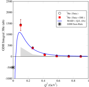
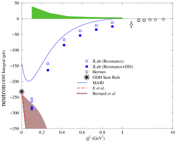
Figure 2: Results for the GDH sum $I(Q^{2})$ for ³He (top) and the neutron (bottom). The ³He GDH results are compared with the MAID model plus a quasielastic contribution. The neutron GDH results are compared with $\chi$PT calculations of ref. [95] (dotted curve) and ref. [97] (dot-dashed curve). The MAID model calculation of ref. [43], is represented by a solid curve. Data from HERMES [64] are also shown.

The ³He results rise with decreasing $Q^{2}$. Since the GDH sum rule at $Q^{2}=0$ predicts a large negative value, a drastic turn around should happen at $Q^{2}$ lower than 0.1 GeV². A simple model using MAID plus quasielastic contributions estimated from a PWIA model [84] indeed shows the expected turn around. The data at low $Q^{2}$ should be a good testing ground for few-body chiral perturbation theory calculations when they are available.

The neutron results indicate a significant yet smooth variation of $I(Q^{2})$ to increasingly negative values as $Q^{2}$ varies from $0.9\,{\rm GeV^{2}}$ towards zero. The data are more negative than the MAID model calculation [43]. Since the calculation only includes contributions to $I(Q^{2})$ for $W\leq 2\,{\rm GeV}$, the model should be compared with the open squares. The GDH sum rule prediction, $I(0)=-232.8\,\mu{\rm b}$, is indicated along with extensions to $Q^{2}>0$ using two next-to-leading order chiral perturbation theory ($\chi$PT) calculations: one of them using the heavy baryon approximation (HB$\chi$PT) [95] (dotted line) and the other relativistic baryon $\chi$PT (RB$\chi$PT) [97] (dot-dashed line). Shown with a brown band is a RB$\chi$PT prediction including resonance effects [97]. The large uncertainty is due to the resonance parameters used.

Improved calculations[98, 99] as well as further measurements [15] will help clarify the situation.

5.3 First moments of $g_{1}$ and the Bjorken sum

The first moment of $g_{1}$, $\Gamma_{1}$, was extracted from E94-010 for the neutron [17] and ³He [19], and from the CLAS eg1 experiment for the proton [22], the deuteron [23] and the neutron (from the deuteron with the proton contribution subtracted) over a $Q^{2}-$range from 0.05 to 5 GeV². The results are plotted in Fig. 3. Also plotted are the results at $Q^{2}=1.3$ GeV² from the Hall C RSS experiment [27]. These moments show a strong yet smooth variation in the transition region ($Q^{2}$ from 1 to 0.05 GeV²). The lowest $Q^{2}$ (0.05-0.1 GeV²) data are compared with two $\chi$PT calculations and are in reasonable agreement.

Also plotted are the preliminary neutron data at very low $Q^{2}$ of 0.04 to 0.24 GeV² from the Hall A E97-110 experiment. The precision of the preliminary data is currently limited by systematic uncertainties, which are expected to be reduced significantly when the final results become available. The new data are in good agreement with published results in the overlap region. The data in the very low $Q^{2}-$region provide a benchmark test of the $\chi$PT calculations, since they are expected to work in this region. The results agree well with both $\chi$PT calculations and also indicate a smooth transition as $Q^{2}$ approaches zero.

The bottom-right panel shows the first moment for p-n [32], a flavor non-singlet combination, which is the Bjorken sum at large $Q^{2}$ [61]. The Bjorken sum was used to extract the strong coupling constant $\alpha_{s}$ at high $Q^{2}$ (5 GeV²). An attempt was made to extract an “effective coupling” $\alpha_{s,g_{1}}$ in the low $Q^{2}-$region using the Bjorken sum, see section 5.9.

At large $Q^{2}$, the data agree with pQCD models where the higher-twist effects are small.

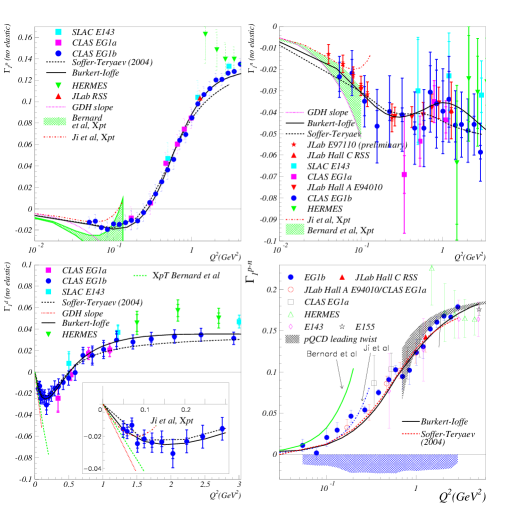
Figure 3: Results of $\Gamma_{1}(Q^{2})$ for p, d, n and p-n from the JLab Hall A, CLAS eg1 and Hall C RSS experiments. The slopes at $Q^{2}=0$ predicted by the GDH sum rule are given by the dotted lines. The dashed (plain) lines are the predictions from the Soffer-Teryaev [100] (Burkert-Ioffe [101] ) model. The leading twist $Q^{2}$-evolution of the moments is given by the gray band. The inset shows comparisons with $\chi$PT calculations by Ji et al. [95] and Bernard et al. [97].

5.4 First moment of $g_{2}$: B-C sum

Measurements of $g_{2}$ require transversely polarized targets. SLAC E155x [74] performed the only dedicated $g_{2}$ measurement prior to JLab. At JLab, $g_{2}$ and its moments have been extensively measured for the neutron with a polarized ³He target in a wide range of kinematics in several Hall A experiments (E94-010 [17], E97-103 [109], E99-117 [110], E02-012 [21] and E97-110 [15]). The measurement on the proton was performed in the RSS experiment in Hall C at an average $Q^{2}$ of 1.3 GeV².

The first moment of $g_{2}$ is expected to be zero at all $Q^{2}$ from the Burkhardt-Cottingham (B-C) sum rule. The SLAC E155x results yielded a first test of the B-C sum rule for the proton, deuteron and neutron (extracted from p and d data). The proton result (top panel of Fig. 4) appears to be inconsistent with the B-C sum rule at the 2.75 $\sigma$ level. In addition to the large experimental uncertainty, there is an uncertainty associated with the low-$x$ extrapolation that is difficult to quantify. The deuteron and neutron (bottom panel of Fig. 4) results from SLAC show agreement with the B-C sum rule with large uncertainties. The most extensive measurements of the B-C sum rule come from experiments [15, 17, 21] on the neutron using a longitudinally and transversely polarized ³He target in Hall A. The results for $\Gamma_{2}^{n}$ are plotted in the bottom panel of Fig. 4 in the measured region (open circles). The solid diamonds include the elastic contribution and an estimated DIS contribution assuming $g_{2}=g_{2}^{WW}$. The published results from E94-010 and the preliminary results from E97-110 and E02-012 are the most precise data on the B-C sum rule and are consistent with the expectation of zero, within small systematic uncertainties. The RSS experiment in Hall C [27] took data on $g_{2}$ for the proton and deuteron, at an average $Q^{2}$ of about 1.3 GeV². For the proton (top panel of Fig. 4), the integral over the measured resonance region is negative, but after the elastic contribution and the estimated small-$x$ part are added, the preliminary result for the B-C sum is consistent with zero. Preliminary result on the deuteron and the neutron (from d and p) are also consistent with zero within uncertainties. The precision data from JLab are consistent with the B-C sum rule in all cases, indicating that $g_{2}$ is a well-behaved function with good convergence at high energy though the high energy part is mostly unmeasured.

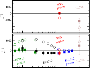
Figure 4: The verification of the BC sum rule from Hall C RSS and Hall A experiments E94-010, E97-110 and E02-012 (neutron only), together with SLAC E155x data. The top plot is for the proton and the bottom for the neutron. The open symbols are the measured values and the solid symbols are the total moments, including the elastic and estimated contributions from the unmeasured high-energy region.

5.5 Spin Polarizabilities: $\gamma_{0}$, $\delta_{LT}$

The generalized spin polarizabilities provide benchmark tests of $\chi$PT calculations at low $Q^{2}$. Since the generalized polarizabilities have an extra $1/\nu^{2}$ weighting compared to the first moments (GDH sum or $I_{LT}$), these integrals have less of a contribution from the large-$\nu$ region and converge much faster, which minimizes the uncertainty due to the unmeasured region at large $\nu$.

At low $Q^{2}$, the generalized polarizabilities have been evaluated with $\chi$PT calculations [96, 105]. One issue in the $\chi$PT calculations is how to properly include the nucleon resonance contributions, especially the $\Delta$ resonance which usually dominates. As was pointed out in Ref. [96, 105], while $\gamma_{0}$ is sensitive to resonances, $\delta_{LT}$ is insensitive to the $\Delta$ resonance. Measurements of the generalized spin polarizabilities are an important step in understanding the dynamics of QCD in the chiral perturbation region.

The first results for the neutron generalized forward spin polarizabilities $\gamma_{0}(Q^{2})$ and $\delta_{LT}(Q^{2})$ were obtained at Jefferson Lab Hall A [18] over a $Q^{2}-$range from 0.1 to 0.9 GeV². We will focus on the low $Q^{2}-$region where the comparison with $\chi$PT calculations is meaningful.

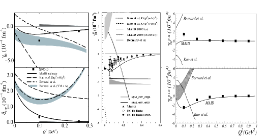
Figure 5: Left panels display results for the neutron spin polarizabilities $\gamma_{0}$ (top) and $\delta_{LT}$ (bottom). Solid squares are the results with statistical uncertainties. The dark bands indicates the systematic uncertainties. The dashed curves are the HB$\chi$PT calculation[105]. The dot-dashed curves and the light bands are the RB$\chi$PT calculation[96] without and with[97] the $\Delta$ and vector-meson contributions, respectively. Solid curves are from the MAID model[43]. The other panels are results for the spin polarizability $\gamma_{0}$ for the proton, $p-n$ and $p+n$.

The results for $\gamma_{0}(Q^{2})$ for the neutron are shown in the top-left panel of Fig. 5 for the two lowest $Q^{2}-$values of 0.10 and 0.26 GeV². The statistical uncertainties are smaller than the size of the symbols. The data are compared with a next-to-leading order, $O(p^{4})$, HB$\chi$PT calculation[105], a next-to-leading-order RB$\chi$PT calculation[96] and the same calculation explicitly including both the $\Delta$ resonance and vector-meson contributions[97]. Predictions from the MAID model[43] are also shown. At the lowest $Q^{2}$ point, the RB$\chi$PT calculation including the resonance contributions agrees with the experimental result. For the HB$\chi$PT calculation without explicit resonance contributions, the discrepancy is large even at $Q^{2}=0.1$ GeV². This might indicate the significance of the resonance contributions or a problem with the heavy baryon approximation at this $Q^{2}$. The higher-$Q^{2}$ data point is in good agreement with the MAID prediction, but the lowest data point at $Q^{2}=0.1$ GeV² is significantly lower, consistent with what was observed for the generalized GDH integral result (Section 5.2). Since $\delta_{LT}$ is insensitive to the dominating $\Delta$-resonance contribution, it was believed that $\delta_{LT}$ should be more suitable than $\gamma_{0}$ to serve as a testing ground for the chiral dynamics of QCD[96, 105]. The bottom-left panel of Fig. 5 shows $\delta_{LT}$ compared to $\chi$PT calculations and the MAID predictions. It is surprising to see that the data are in significant disagreement with the $\chi$PT calculations even at the lowest-$Q^{2}$ of 0.1 GeV². This discrepancy presents a significant challenge to the present theoretical understanding. The MAID predictions are in good agreement with the results.

The other panels of Fig. 5 present results of $\gamma_{0}$ for the proton [25] and for the isospin decompositions: p-n and p+n [32].

These results are in strong disagreements with both $\chi$PT calculations. Since $\gamma_{0}$ is sensitive to the $\Delta$ contributions, this may indicate that the treatment of the $\Delta$ contributions in the $\chi$PT calculations needs to be taken into account properly. Progress in this direction is expected in the near future [98].

5.6 Higher moment $d_{2}$ and higher twist: twist-3

Another combination of the second moments, $d_{2}(Q^{2})$, provides an efficient way to study the high-$Q^{2}$ behavior of nucleon spin structure, since at high $Q^{2}$ it is related to a matrix element $d_{2}$ (color polarizability) which can be calculated from Lattice QCD. This moment also provides a means to study the transition from high to low $Q^{2}$. In the left panel of Fig. 6, $\bar{d}_{2}(Q^{2})$ on the neutron is shown. The preliminary results from E02-012 [21] and the published E94-010 [17] results are shown as the solid squares and open circles, respectively. The bands represent the systematic uncertainties. The neutron results from SLAC[74](open diamond) at high $Q^{2}$ and from combined SLAC and JLab E99-117[110](solid diamond) are also shown. The solid line is the MAID calculation containing only the resonance contribution. At moderate $Q^{2}$, our data show that $\bar{d}_{2}^{n}$ is positive and decreases with $Q^{2}$. At large $Q^{2}$ ($Q^{2}=5$ GeV²), data (SLAC alone and SLAC combined with JLab E99-117) are positive. The lattice QCD prediction[106] at $Q^{2}=5$ GeV² is negative but close to zero and is about two sigmas away from the data. We note that all models (not shown at this scale) predict a small negative or zero value at large $Q^{2}$. High-precision data at large $Q^{2}$ will be crucial for a benchmark test of the lattice QCD predictions and for understanding the dynamics of the quark-gluon correlations.

file=d2n.eps, scale=0.45 file=d2p.eps, scale=0.30

Figure 6: The left plot shows the Hall A results of $\overline{d}_{2}$ for the neutron along with the world data at high $Q^{2}$, Lattice QCD, MAID model and HB$\chi$PT calculations. The right plot shows the Hall C result of $\overline{d}_{2}$ for the proton at $Q^{2}=1.3$ GeV², the same data evolved to $Q^{2}=5$ GeV² along with the SLAC data and lattice QCD calculation.

Also shown are the $d_{2}$ result on the proton from Hall C [28] at $Q^{2}=1.3$ GeV² and the same result evolved to $Q^{2}=5$ GeV² along with the SLAC data and the Lattice QCD calculation.

5.7 Higher twist extractions: $f_{2}$, twist-4

The higher-twist contributions to $\Gamma_{1}$ can be obtained by a fit with an OPE series, Eq. (59), truncated to an order appropriate for the precision and $Q^{2}$-span of the data. The goal is to determine the twist-4 matrix element $f_{2}$. Once $\mu_{4}$ is obtained, $f_{2}$ is extracted by subtracting the leading-twist contributions of $a_{2}$ and $d_{2}$ following Eq. (62). The data precision and $Q^{2}-$range allow a fit to both the $\mu_{4}$ and $\mu_{6}$ terms. To have an idea how the higher-twist terms (twist-8 and above) affect the twist-4 term extraction, it is necessary to study the convergence of the expansion and to choose the $Q^{2}-$range in a region where the $\mu_{8}$ term is not significant. A fit with three terms ($\mu_{4}$, $\mu_{6}$ and $\mu_{8}$) was also preformed for this purpose. This study was possible only because of the availability of the high-precision low-$Q^{2}$ data from JLab.

Higher-twist analyses have been performed on the proton[31], the neutron[29] and the Bjorken sum[32]. An earlier proton analysis is available[30] but will not be presented here, since that analysis used a different procedure. $\Gamma_{1}$ at moderate $Q^{2}$ is obtained as described in section 5.1. For consistency, the unmeasured low-$x$ parts of the JLab $\Gamma_{1}^{p}$ and of the world data on $\Gamma_{1}$ were re-evaluated using the same prescription previously used for $\Gamma_{1}^{n}$ and $\Gamma_{1}^{p-n}$. The elastic contribution, negligible above $Q^{2}$ of 2 GeV² but significant (especially for the proton) at lower values of $Q^{2}$, was added using the parametrization of Ref. [103]. The leading-twist term $\mu_{2}$ was determined by fitting the data at $Q^{2}\geq 5$ GeV² assuming that higher twists are negligible in this $Q^{2}-$region. A value of $g_{A}=1.270\pm 0.045$ was obtained for the Bjorken sum. Using the proton (neutron) data alone, and with input of $g_{A}$ from neutron beta decay and $a_{8}$ from hyperon decay (assuming SU(3) flavor symmetry), we obtained $\Delta\Sigma=0.15\pm 0.07$ for the proton and $\Delta\Sigma=0.35\pm 0.08$ for the neutron. We note that there is a significant difference between $\Delta\Sigma$ determined from the proton and from the neutron data. This is the main reason why the extracted $\mu_{4}$ and $f_{2}$ from the Bjorken sum is different compared to the difference of those extracted individually from the proton and neutron, since the Bjorken sum does not need the assumption of SU(3) flavor symmetry and $\Delta\Sigma$ was canceled.

The fit results using an expansion up to ($1/Q^{6}$) in determining $\mu_{4}$ are summarized in Table 1. In order to extract $f_{2}$, as shown in Table 2, the target-mass corrections $a_{2}$ were evaluated using the Blumlein-Boettcher world data parametrization[108] for the proton and a fit to the world neutron data, which includes the recent high-precision neutron results at large $x$[110]. The $d_{2}$ values used are from SLAC E155x[74] (proton) and JLab E99-117[110] (neutron).

Results of $\mu_{4}$, $\mu_{6}$ and $\mu_{8}$ at $Q^{2}$ = 1 GeV² for proton, neutron and $p-n$. The uncertainties are first statistical, then systematic. Target $Q^{2}$ (GeV²) $\mu_{4}/M^{2}$ $\mu_{6}/M^{4}$ $\mu_{8}/M^{6}$ proton 0.6-11.0 -0.065$\pm 0.012\pm 0.048$ 0.143$\pm 0.021\pm 0.056$ -0.026$\pm 0.008\pm 0.016$ neutron 0.5-11.0 0.019$\pm 0.002\pm 0.024$ -0.019$\pm 0.002\pm 0.017$ 0.00$\pm 0.00\pm 0.03$ $p-n$ 0.5-11.0 -0.060$\pm 0.045\pm 0.018$ 0.086$\pm 0.077\pm 0.032$ 0.011$\pm 0.031\pm 0.019$

Results of $f_{2}$, $\chi_{E}$ and $\chi_{B}$ at $Q^{2}$ = 1 GeV² for proton, neutron and $p-n$. The uncertainties are first statistical, then systematic. Target $f_{2}$ $\chi_{E}$ $\chi_{B}$ $p$ -0.160 $\pm 0.028\pm 0.109$ -0.082 $\pm 0.016\pm 0.071$ 0.056 $\pm 0.008\pm 0.036$ $n$ 0.034 $\pm 0.005\pm 0.043$ 0.031 $\pm 0.005\pm$ 0.028 -0.003 $\pm$ 0.004 $\pm$ 0.014 $p-n$ $-0.136\pm 0.102\pm 0.039$ $-0.100\pm 0.068\pm 0.028$ $0.036\pm 0.034\pm 0.017$

The $\Gamma_{1}$ moments were fit, varying the minimum $Q^{2}-$value to study the convergence of the OPE series. The extracted quantities have large uncertainties (dominated by the systematic uncertainty) but are stable with respect to a minimal $Q^{2}-$value when it is below 1 GeV². The results do not vary significantly when the $\mu_{8}$ term is added, which justifies a posteriori the use of the truncated OPE series in the chosen $Q^{2}-$range. In the proton case, the elastic contribution makes a significant contribution to the $\mu_{6}$ term at low $Q^{2}$ but this does not invalidate a priori the validity of the series since the elastic contributes mainly to $\mu_{6}$ and $\mu_{8}$, but remains small compared to $\mu_{4}$. We notice the alternation of signs between the coefficients. This leads to a partial suppression of the higher-twist effects and may be a reason for quark-hadron duality in the spin sector[111]. We also note that the sign alternation is opposite for the proton and neutron. Following Eq. (73), the electric and magnetic color polarizabilities were determined. Overall, the values given in Table 2 are small, and we observe a sign change in the electric color polarizability between the proton and the neutron. We also expect a sign change in the color magnetic polarizability. However, with the large uncertainty and the small negative value of the neutron $\chi_{B}$, it is difficult to confirm this expectation.

5.8 Quark-hadron duality in spin structure functions

Detailed studies of duality in the spin structure functions $g_{1}^{p}$ and $g_{1}^{d}$ have been published by the CLAS eg1 [26] collaboration. One observes a clear trend of strong, resonant deviations from the scaling curve at lower $Q^{2}$ towards a pretty good agreement at intermediate $Q^{2}$. The integral of $g_{1}$ over the whole resonance region begins to agree with the NLO results above $Q^{2}\approx 1.7$ GeV² (see Fig. 7). The results on the proton and deuteron from eg1b [26] thus indicate a much slower approach to “global” duality for the polarized structure function $g_{1}$ than has been observed for the unpolarized structure functions [111] Local duality seems violated in the $\Delta-$resonance region even for $Q^{2}-$values as high as 5 GeV².

The data taken by the RSS collaboration in Hall C [27] corroborate these observations and add more precise data points for $Q^{2}\approx 1.3$ GeV².

file=dualgamma1.eps, scale=0.34 file=gamma1_duality.eps, scale=0.38

Figure 7: Data on $g_{1}(x,Q^{2})$ averaged over the resonance region for the proton and the deuteron from Hall B eg1 (left panel). The hatched curves represent the range of extrapolated DIS results from modern NLO fits (GRSV and AAC), evolved to the $Q^{2}$ of the data and corrected for target mass effects. The open circles in the left panel include the elastic contribution, while the filled circles are only integrated over $W>1.08$ GeV. The right panel shows $\Gamma_{1}^{3He}$ and $\Gamma_{1}^{n}$ of the resonance region from Hall A E01-012, together with lower $Q^{2}$ results from E94-010, compared with the world DIS fits.

The spin structure functions $g_{1}$ and $A_{1}$ were measured in the resonance region ($W<2$ GeV) for ³He in the $Q^{2}-$region below 1 GeV² by Hall A experiments E94-010 [17, 19] and from 1 GeV² to 4 GeV² by E01-012 [20]. Due to the prominent contributions from the $\Delta$ resonance, local duality does not appear to work at low $Q^{2}$ (below 2 GeV²). At high $Q^{2}$ (above 2 GeV²), the $\Delta$-resonance contribution starts to diminish. The resonance data were integrated to study global duality. Figure 7 (right panel) shows the results for both ³He and the neutron in comparison with the DIS fits evolved to the same $Q^{2}$. The resonance data agree with the DIS fits at least for $Q^{2}$ higher than 1.8 GeV², indicating that global duality holds for the neutron and ³He spin structure function, $g_{1}$, in the high $Q^{2}-$region (above 1.8 GeV²).

The study of quark-hadron duality helps us to study higher-twist effects and decide where to extend the kinematic region apply partonic interpretations. From a practical point of view, the good understanding of the higher twist effects and quark-hadron duality allows us to considerably extend the experimental database used to extract the polarized parton distributions [112].

5.9 The effective strong coupling at large distance

In QCD, the magnitude of the strong force is given by the running coupling constant $\alpha_{s}$. At large $Q^{2}$, in the pQCD domain, $\alpha_{s}$ is well defined and can be experimentally extracted, e.g. using the Bjorken sum rule, (see eq. 61). The pQCD definition leads to an infinite coupling at large distances, where $Q^{2}$ approaches $\Lambda^{2}_{QCD}$, This is not a conceptual problem because we are out of the validity domain of pQCD. Since the data show no sign of discontinuity when crossing the intermediate $Q^{2}-$domain, see e.g. Fig. 3, it is natural to look for a definition of an effective coupling $\alpha_{s}^{eff}$, which works at any $Q^{2}$ and matches $\alpha_{s}$ at large $Q^{2}$ but stays finite at small $Q^{2}$. The Bjorken sum rule can be used advantageously to define $\alpha_{s}^{eff}$ at low Q² [113]. The data on the Bjorken sum are used to experimentally extract $\alpha_{s}^{eff}$ following a prescription by Grunberg [114], see Fig. 8. The Bjorken and GDH sum rules also allow us to determine $\alpha_{s}^{eff}$ at, respectively, large $Q^{2}$ and $Q^{2}\simeq 0$. The extracted $\alpha_{s}^{eff}$ provides for the first time an experimental “effective coupling” at all $Q^{2}$. An interesting feature is that $\alpha_{s}^{eff}$ becomes scale invariant at small $Q^{2}$, which was predicted by a number of calculations.

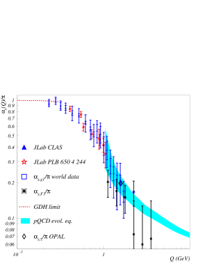
Figure 8: Value of $\alpha_{s}^{eff}/\pi$ extracted from the data on the Bjorken sum, on $\tau$ decay and on the Gross-Llewellyn-Smith sum. The values of $\alpha_{s}^{eff}$ computed within pQCD and using the Bjorken sum are given by the gray band. The values of $\alpha_{s}^{eff}/\pi$ extracted using the GDH sum rule are given by the red dashed line.

6 Conclusion

A large body of nucleon spin-dependent cross-section and asymmetry data have been collected at low to moderate $Q^{2}$ in the resonance region. These data have been used to evaluate the $Q^{2}-$dependence of moments of the nucleon spin structure functions $g_{1}$ and $g_{2}$, including the GDH integral, the Bjorken sum, the BC sum and the spin polarizabilities, and to extract higher-twist contributions. The latter have provided access to the color polarizabilities in the nucleon.

At $Q^{2}$ close to zero, available next-to-leading order $\chi$PT calculations were tested against the data and found to be in reasonable agreement for $Q^{2}$ = 0.1 GeV² for the GDH integral $I(Q^{2})$ and $\Gamma_{1}(Q^{2})$. Above $Q^{2}$ = 0.1 GeV² a significant difference between the calculation and the data is observed, pointing to the limit of applicability of $\chi$PT as $Q^{2}$ becomes larger. The comparison of results for the forward spin polarizabilities $\gamma_{0}(Q^{2})$ and $\delta_{LT}$ with the $\chi$PT calculations show significant disagreements. $\gamma_{0}(Q^{2})$ has significant contributions from the $\Delta$ resonance and its inclusion in $\chi$PT calculations have not been fully worked out. The disagreements may indicate a better treatment of the $\Delta$ resonance is needed in the $\chi$PT calculations. On the other hand, the $\chi$PT calculation of $\delta_{LT}$ was expected to offer a faster convergence because of the absence of the $\Delta$ contribution. However, none of the available $\chi$PT calculations can reproduce $\delta_{LT}$ for the neutron at the lowest $Q^{2}$ point of 0.1 GeV². This discrepancy presents a significant challenge to our theoretical understanding at its present level of approximations.

Overall, the trend of the data is well described by phenomenological models. The dramatic $Q^{2}-$evolution of $I_{GDH}$ from high to low $Q^{2}$ was observed as predicted by these models for both the proton and the neutron. This behavior is mainly determined by the relative strength and sign of the $\Delta$ resonance compared to that of higher-energy resonances and deep-inelastic processes. This also shows that the current level of phenomenological understanding of the resonance spin structure using these moments as observables is reasonable.

The neutron BC sum rule is observed to be verified within experimental uncertainties in the low-$Q^{2}$ region due to a cancellation between the inelastic and the elastic contributions. The BC sum rule is expected to be valid at all $Q^{2}$. This test validates the assumptions going into the BC sum rule, which provides confidence in sum rules with similar assumptions.

In the $Q^{2}$-region above 0.5 GeV², the first moment of $g_{1}$ for the proton, neutron and the proton-neutron difference were re-evaluated using the world data and the same extrapolation method of the unmeasured regions for consistency. Then, in the framework of the OPE, the higher-twist $f_{2}$ and $d_{2}$ matrix elements were extracted. The low-$Q^{2}$ data have allowed us to gauge the convergence of the expansion used in this analysis. The extracted higher-twist (twist-4 and above) effects are not significant for $Q^{2}$ above 1 GeV². This fact may be related to the observation that quark-hadron duality works reasonably well at Q² above 1 GeV².

Finally, the proton and neutron electric and magnetic color polarizabilities were determined by combining the twist-4 matrix element $f_{2}$ and the twist-3 matrix element $d_{2}$ from the world data. Our findings show a small and slightly positive value of $\chi_{E}$ and a value of $\chi_{B}$ close to zero for the neutron, while the proton has slightly larger values for both $\chi_{E}$ and $\chi_{B}$ but with opposite signs.

Overall, the new JLab data have provided valuable information on the transition between the non-perturbative to the perturbative regime of QCD. They form a precise data set for twist expansion analysis and a check of $\chi$PT calculations.

Recently completed measurements [115, 116] and future 12 GeV experiments [115] on the $g_{1}$, $g_{2}$ structure functions and $d_{2}$ moments for the proton and neutron at $Q^{2}\approx 1-5$ GeV² will reduce the uncertainty in the extracted higher-twist coefficients and provide a benchmark test of Lattice QCD.

References

- [1] V. Bernard, Prog. Part. Nucl. Phys. 60, 82 (2008).
- [2] M. Gockeler et al., PoS LAT2006, 120 (2006).
- [3] I. C. Cloet and C. D. Roberts, PoS LC2008, 047 (2008).
- [4] See, e.g., J. Polchinski and M. J. Strassler, Phys. Rev. Lett. 88, 031601 (2002); ibid. S. J. Brodsky and G. F. de Teramond, Phys. Rev. Lett. 96, 201601 (2006); 94, 201601 (2005).
- [5] E. V. Shuryak and A. I. Vainshtein, Nucl. Phys. B 201, 141 (1982).
- [6] E. Stein, P. Gornicki, L. Mankiewicz and A. Schäfer, Phys. Lett. B 353, 107 (1995).
- [7] X. Ji, Nucl. Phys. B 402, 217 (1993).
- [8] O. Stern and W. Gerlach, Z. Physik 7, 249 (1921); ibid., 8, 110 (1921); ibid., 9, 349 and 353 (1922).
- [9] R. Frisch and O. Stern, Z. Physik 85, 4 (1933); I. Estermann and O. Stern, ibid., 7 (1933).
- [10] S. B. Gerasimov, Sov. J. Nucl. Phys. 2, 598 (1965)
- [11] S. D. Drell and A. C. Hearn, Phys. Rev. Lett. 16, 908 (1966).
- [12] R. Hofstadter, Rev. Mod. Phys. 28, 214 (1956).
- [13] See, e.g., S. E. Kuhn, J. -P. Chen and E. Leader, Prog. Part. Nucl. Phys., 63, 1 (2009).
- [14] J. D. Bjorken, Phys. Rev. 148, 1467 (1966).
- [15] JLab E97-110, J. P. Chen, A. Deur, F. Garibaldi, spokespersons; V. Sulkosky, Proc. Spin Structure at Long Distance, Edited by J. P. Chen, W. Melnitchouk and K. Slifer, AIP 1151, 93 (2009).
- [16] M. Amarian et al., Phys. Rev. Lett. 89, 242301 (2002).
- [17] M. Amarian et al., Phys. Rev. Lett. 92, 022301 (2004).
- [18] M. Amarian et al., Phys. Rev. Lett. 93, 152301 (2004).
- [19] K. Slifer et al., Phys. Rev. Lett. 101, 022303 (2008).
- [20] P. Solvignon et al., Phys. Rev. Lett. 101, 182502 (2008).
- [21] P. Solvignon, Proc. Spin Structure at Long Distance, Edited by J. P. Chen, W. Melnitchouk and K. Slifer, AIP 1151, 101 (2009).
- [22] R. Fatemi et al., Phys. Rev. Lett. 91, 222002 (2003).
- [23] J. Yun et al., Phys. Rev. C 67, 055204 (2003).
- [24] K. V. Dharmawardane et al., Phys. Lett. B 641, 11 (2006).
- [25] Y. Prok et al., Phys. Lett. B 672, 12 (2009).
- [26] P. Bosted et al., Phys. Rev. C 75, 035203 (2007).
- [27] F. R. Wesselmann et al., Phys. Rev. Lett. 98, 132003 (2007).
- [28] K. Slifer et al., arXiv nucl-ex/08120031.
- [29] Z.-E. Meziani et al., Phys. Lett. B 613, 148 (2005).
- [30] M. Osipenko et al., Phys. Lett. B 609, 259 (2005).
- [31] A. Deur, arXiv nucl-ex/0508022.
- [32] A. Deur et al., Phys. Rev. Lett. 93, 212001 (2004); A. Deur et al., Phys. Rev. D 78, 032001 (2008).
- [33] J. Ahrens et al. Phys. Rev. Lett. 87, 022003 (2001).
- [34] H. Dutz et al., Phys. Rev. Lett. 91, 192001 (2003).
- [35] H. Dutz et al., Phys. Rev. Lett. 93, 032003 (2004).
- [36] M. Anselmino, A. Efremov and E. Leader, Phys. Rep. 261, 1 (1995); ibid., 281 399 (erratum) (1997).
- [37] J. Soffer, O. V. Teryaev, arXiv hep-ph/9906455.
- [38] X. Artru, M. Elchikh, J. M. Richard, J. Soffer and O. V. Teryaev, hep-ph/08020164.
- [39] D. Drechsel and T. Walcher, Rev. Mod. Phys. 80, 731 (2008).
- [40] L. N. Hand, Phys. Rev. 129, 1834 (1963).
- [41] P. Hoodbhoy, R. L. Jaffe and A. Manohar, Nucl. Phys. B 312, 571 (1989).
- [42] L. L. Frankfurt and M. I. Strikman, Nucl. Phys. A 405, 557 (1983).
- [43] D. Drechsel, S.S. Kamalov and L. Tiator, Phys. Rev. D 63, 114010 (2001).
- [44] X. Ji and J. Osborne, J. of Phys. G 27, 127 (2001).
- [45] M. Anselmino, B. L. Ioffe, and E. Leader, Sov. J. Nucl. Phys. 49, 136 (1989).
- [46] D. Drechsel, B. Pasquini and M. Vanderhaeghen, Phys. Rep. 378, 99 (2003).
- [47] D. Drechsel and L. Tiator, Ann. Rev. Nucl. Part. Sci. 54, 69 (2004).
- [48] J. D. Bjorken and S. D. Drell, “Relativistic Quantum Fields”, McGraw Hill, New York (1965).
- [49] F. E. Low, Phys. Rev. 96, 1428 (1954).
- [50] K. Wilson, Phys. Rev. 179, 1499 (1969).
- [51] H. Burkhardt and W. N. Cottingham, Ann. Phys. (N.Y.) 56, 453 (1970).
- [52] J. Ellis and R. L. Jaffe, Phys. Rev. D 9, 1444 (1974); ibid., D 10, 1669 (1974).
- [53] X. Ji and P. Unrau, Phys. Lett. B 333, 228 (1994).
- [54] X. Ji and W. Melnitchouk, Phys. Rev. D 56,1 (1997).
- [55] S. Wandzura and F. Wilczek, Phys. Lett. B 72, 195 (1977).
- [56] M. Burkardt, Proc. Spin Structure at Long Distance, Edited by J. P. Chen, W. Melnitchouk and K. Slifer, AIP 1151, 26 (2009).
- [57] J. Ashman et al., Phys. Lett. B 206, 364 (1988).
- [58] SMC collaboration: D. Adams et al., Phys. Lett. B 329, 399 (1994).
- [59] SMC collaboration: D. Adams et al., Phys. Lett. B 357, 248 (1995).
- [60] SMC collaboration: D. Adams et al., Phys. Lett.B 396, 338 (1997).
- [61] SMC collaboration: D. Adeva et al., Phys. Lett. B 302, 533 (1993).
- [62] SMC collaboration: D. Adeva et al., Phys. Lett.B 412, 414 (1997).
- [63] K. Ackerstaff et al., Phys. Lett. B 404, 383 (1997).
- [64] K. Ackerstaff et al., Phys. Lett. B 444, 531 (1998).
- [65] A. Airapetian, et al., Phys. Lett. B 442, 484 (1998).
- [66] M. J. Alguard et al., Phys. Rev. Lett. 37, 1261 (1976).
- [67] M. J. Alguard et al., Phys. Rev. Lett. 41, 70 (1976).
- [68] P. L. Anthony et al., Phys. Rev. D 54, 6620 (1996).
- [69] K. Abe et al., Phys. Rev. D 58,112003 (1998).
- [70] K. Abe et al., Phys. Rev. Lett. 79, 26 (1997).
- [71] K. Abe et al., Phys. Lett. B 404, 377 (1997).
- [72] P. L. Anthony, et al., Phys. Lett. B 493, 19 (2000).
- [73] P. L. Anthony, et al., Phys. Lett. B 458, 529 (1999).
- [74] P. L. Anthony et al., Phys. Lett. B 553, 18 (2003).
- [75] C. Bernet, Proceedings of DIS2005 (2005), Madison, Wisconsin, AIP Conf. Proc. (2005).
- [76] A. Deshpande, Proceedings of DIS2005 (2005), Madison, Wisconsin, AIP Conf. Proc. (2005).
- [77] X. Ji, Phys. Rev. Lett. 78, 610 (1997).
- [78] M. Burkardt, Phys. Rev. D 72, 094020 (2005).
- [79] Hall A collaboration: J. Alcorn et al., Nucl. Inst. Meth. A522, 294 (2004).
- [80] Hall A Status Report - 2007.
- [81] CLAS collaboration: B. A. Mecking et al., Nucl. Inst. Meth. A503, 513 (2003).
- [82] L.W. Mo and Y.S. Tsai, Rev. Mod. Phys. 41, 205 (1969).
- [83] I.V Akushevich and N.M. Shumeiko, J. Phys. G 20, 513 (1994).
- [84] C. Ciofi degli Atti and S. Scopetta, Phys. Lett. B 404, 223 (1997).
- [85] A. Abragam and M. Goldman, Rep. Prog. Phys. 41 396 (1978).
- [86] D.G. Crabb and W. Meyer, Annu. Rev. Nucl. Part. Sci. 47, 67 (1997).
- [87] C. D. Keith et al., Nucl. Inst. Meth. A 501, 327 (2003).
- [88] L.W. Whitlow et al., Phys. Lett. B 250, 193 (1990);
- [89] Y. Liang et al., nucl-ex/0410027.
- [90] K. Abe et al., Phys. Rev. D 58 112003 (1998).
- [91] M. Arneodo et al., Phys. Lett. B 364, 107 (1995).
- [92] V. Burkert and Z. Li, Phys. Rev D 47, 46 (1993).
- [93] J. Soffer, Phys. Rev. Lett. 74, 1292 (1995).
- [94] N. Bianchi and E. Thomas, Nucl. Phys. B 82 (Proc. Suppl.), 256 (2000).
- [95] X. Ji, C. Kao, and J. Osborne, Phys. Lett. B 472, 1 (2000).
- [96] V. Bernard, T. Hemmert and Ulf-G. Meissner, Phys. Lett. B 545, 105 (2002)
- [97] V. Bernard, T. Hemmert and Ulf-G. Meissner, Phys. Rev. D 67, 076008 (2003).
- [98] H. Krebs, et al., Proc. Spin Structure at Long Distance, Edited by J. P. Chen, W. Melnitchouk and K. Slifer, AIP 1151, 42 (2009).
- [99] C. W. Kao, Proc. 18th Int. Spin Phys. Symp. Edited by D. Crabb, et al., AIP 1149, 289 (2008).
- [100] J. Soffer and O. V. Teryaev, Phys. Rev. D 70, 116004 (2004).
- [101] V. D. Burkert and B. L. Ioffe, Phys. Lett. B 296, 223 (1992).
-
[102]
The Science Driving the 12 GeV Upgrade of CEBAF,
http://www.jlab.org/div_dept/physics_division/GeV.html. - [103] P. Mergell, Ulf-G. Meissner and D. Drechsel, Nucl. Phys. A 596, 367 (1996).
- [104] S. A. Kulagin and W. Melnitchouk (to be published), private communication.
- [105] C. W. Kao, T. Spitzenberg and M. Vanderhaeghen, Phys. Rev. D 67, 016001 (2003).
- [106] M. Gockeler et al., Phys. Rev. D 63, 074506, (2001).
- [107] V. D. Burkert, Phys. Rev. D 63, 097904 (2001).
- [108] J. Blumlein and H. Boettcher, Nucl. Phys. 636, 225 (2002).
- [109] K. Kramer et al., Phys. Rev. Lett. 95, 142002 (2005).
- [110] X. Zheng et al., Phys. Rev. C 70, 065207 (2004).
- [111] W. Melnitchouk, R. Ent and C. Keppel, Phys. Rept. 406, 127 (2005).
- [112] E. Leader, A. V. Sidorov, D. B. Stamenov, Phys. Rev. D 63, 034023 (2006).
- [113] A. Deur, V. Burkert, J. P. Chen and W. Korsch, Phys. Lett. B 665, 349 (2008);B 650, 244 (2007).
- [114] G. Grunberg, Phys. Lett. B 95, 70 (1980); Phys. Rev. D 29, 2315 (1984); Phys. Rev. D 40, 680 (1989).
- [115] B. Sawatzky et al., Proc. Spin Structure at Long Distance, Edited by J. P. Chen, W. Melnitchouk and K. Slifer, AIP 1151, 145 (2009).
- [116] O. A. Randon, Proc. Spin Structure at Long Distance, Edited by J. P. Chen, W. Melnitchouk and K. Slifer, AIP 1151, 82 (2009).