A statistical mechanics approach
to autopoietic immune networks

Chapter 1 Introduction

1.1 Preface

The aim of this work is to try to bridge over theoretical immunology and disordered statistical mechanics. Our long term hope is to contribute to the development of a quantitative theoretical immunology from which practical applications may stem.

In order to make theoretical immunology appealing to the statistical physicist audience we are going to work out a research article which, from one side, may hopefully act as a benchmark for future improvements and developments, from the other side, it is written in a very pedagogical way both from a theoretical physics viewpoint as well as from the theoretical immunology one.

Furthermore, we have chosen to test our model describing a wide range of features of the adaptive immune response in only a paper: this has been necessary in order to emphasize the benefit available when using disordered statistical mechanics as a tool for the investigation. However, as a consequence, each section is not at all exhaustive and would deserve deep investigation: for the sake of completeness, we restricted details in the analysis of each feature with the aim of introducing a self-consistent model.

1.2 Immune system and statistical mechanics

The purpose of the immune system is to detect and neutralize the molecules, or cells, dangerous for the body (antigens, which could be foreign invaders - e.g. viruses or bacteria - or deranged - e.g. cancerous - cells of the host), without damaging healthy cells [9]. Despite of the evident differences, to accomplish its function, the immune system exhibits properties analogous to the nervous system [45]: it "learns" not to attack healthy cells and it "develops a memory" of the pathogens encountered as time goes by. In theoretical immunology there are two main strands to explain the functioning of the immune system that ultimately represent two approaches, reductionist and systemic for the modeling of nature in general. In the first and most popular approach, lymphocytes basically operate independently or, better, the researcher focuses on the action of the single lymphocyte and on the details of its interactions (i.e. internal cascade signals, etc.) rather than on the global behavior of all the lymphocytes interacting with each other. In the second approach, pioneered in immunology by Elrich [6] and Jerne [32], the immune system is thought of as a whole and designed as a network of cells stimulated to proliferate by the affinity interactions of their exchanging antibodies (a functional idiotypic network [22]). Interestingly, the two approaches are not incompatible but complementary. While the former deals primarily with the response to a stimulus, the latter allows to explain the ability to learn and memorize of the immune system and the tolerance to low doses of antigen [61]. In the past, the immune network theory has been investigated, although not exhaustively, with disordered statistical mechanics tools [25]. However, recent and deep advances in the field of statistical mechanics of highly diluted networks [17, 37, 50, 52, 54, 59] now allow to combine the two viewpoints described above and to develop a unified and quantitative theory. Indeed, reductionist and systemic approaches can be recovered as special cases of null and not-negligible connectivity respectively. This unification should be extremely promising from a biological as well as mathematical point of view.

To sketch our viewpoint on the systemic approach we make the following parallel: the immunologist wonders about the details, even “hyperfine”, of the structure and about the interaction of the lymphocyte with its “particular environment”. Analogously, the condensed matter physicist studies the molecule of water in every detail, from the angle between hydrogen atoms to the constructive interference between the orbital of hydrogen and of oxygen. This speculation is fundamental, yet not exhaustive. In fact, from these details, which allow an accurate description of the molecule, we are not able to deduce, the "emerging properties of the network" of molecules (e.g. a water-ice phase transition) as the control parameters (pressure and temperature) are tuned. Indeed, these phenomena do not depend significantly on the details of the molecule structure but rather on the collective effects due to the interactions of large numbers of these molecules and the study of such effects is just the goal of statistical mechanics. Hence, within this framework, we want to read the theory of the immune networks.

In a nutshell, statistical mechanics (for discrete systems as the one considered here, i.e. Curie-Weiss theories [14, 18, 51] and their complex generalizations [12, 15, 16, 58]) is a powerful approach to this problem. Within the one-body interaction with the external stimuli, it can describe the behavior of the single clone (made up of a set of identical lymphocytes) with its coupled antigen, while, with the two-body interaction, it can describe the clone networks; in this way, interpolating between the two, we can recover the two prototypes of theoretical immunology; furthermore this approach is strongly based on probability theory and on physical variational principles which allow to make the theory even quantitative and predictive.

Turning to the object of application, immunology became so far one of the most investigated field of science and the plethora of its variegate scientific outcomes increases enormously year by year, such that trials for a general unifying theory should be attempted.

We start by introducing the one-body theory and noticing that in immunology it corresponds to what we call a “Burnet-like behavior”, then we extend our model including the two-body theory and show that it recovers what we call a “Jerne-like behavior”; as a natural consequence, we will show how this extends the approach of Counthino-Varela for the systemic self/non-self distinction [27, 28]. After these results, we show how hysteresis, with its remanent magnetization, can play the role of the generator of memory cells from plasma cells, according to the Clonal Selection Theory [4, 5]. Finally, we show how low- and high-dose tolerances, as well as the bell-shaped response, appear as emergent features in our model, while in theoretical immunology analysis they are often postulated a-priori.

Even though not exhaustive, our model may act as an alternative starting backbone for this field of research.

1.3 Theoretical immunology through complex system glasses

The immune system exhibits an extremely broad ensemble of characters, however we are going to focus just on a subset of the whole system, namely the one constituted by B lymphocytes and their related immunoglobulins. Despite being a small part of the immune system, it is the main constituent of the adaptive response and, basically, the core of the system; furthermore, similar considerations may hold, with little modifications, even for the T-killer response, ultimately the adaptive system as a whole (apart from the fundamental T-helper regulations, which from disordered statistical mechanics viewpoint are closer to pure glassy models and quite different from the scenario we propose here, see [25]).

In the following, no mention to any other element (neutrophils, macrophages, APC, etc) will be made and we refer to specialized textbooks for their introduction [9], although their knowledge is not a prerequisite for reading the manuscript.

Let us just sketch, for the sake of clearness, that we are trying to model the B-core of the immune system (as well as the T-killer core) as imitative, eliciting, models: Stimulation is expressed by a firing lymphocyte towards its nearest neighbors while suppression is expressed by a quiescent one. Hence, in our scheme, it is not the sign of the coupling to establish the kind of interaction, i.e. positive for imitative interaction and negative for anti-imitative interaction, which here is always positive or zero, but the state of the single lymphocyte itself.

Frustration surely is expected to appear in the immune system, but, in our approach, it is encoded into the T-helper regulation of the two core (B, T-killers) responses, which deserve another work for its investigation.

1.3.1 Clonal expansion and one body perspective

The main constituents of an (adaptive) immune system are B-lymphocytes (B-cells), together with the T-lymphocytes, and free antibodies produced by B-cells. B-cells and T-cells have specific protein molecules on their surfaces, called receptors. The receptors of B-cells are antibodies (Immunoglobulin, Ig), which can recognize and connect to antigens in order to neutralize them. Finally, the purpose of killer T-cells is to attack and kill infected or deranged cells. The receptors of B- and T-cells have specific $3$-dimensional structures, called “idiotypes”. A family of B-cells generated by a proliferating B-cell are called “clones”; a clone and the antibodies which it produces have the same idiotypes.

In a healthy human body at rest, it is estimate that the total number of "sentinel" clones generated from a single B-cell (the amount of identical lymphocytes) is about $10^{2}$ to $10^{4}$, the total number of clones amounts to some $10^{12}-10^{14}$ (such that diverse clones are around $10^{10}-10^{12}$, and the number of antibodies is about $10^{18}$; remarkably the amount of epitopes/idiotopes belonging to a given antibody are present in a smaller number, i.e. order of $10^{2}$.

When antigens enter the body, those clones which recognize it will bind to it. Aided by helper T-cells, B-cells of an activated clone will proliferate, becoming antibody producing cells. The latter will secrete large numbers of free antibodies, which attach to antigen, neutralize it, and trigger killer cells into action. The above is (a part of the) "clonal selection theory" and has been confirmed experimentally.

We notice that this approach, pioneered by Burnet [4], takes into account an enormous amount of different data, and absolutely does not rely on interactions among different lymphocytes, as it deals with the external antigen interaction with the immune system, where the network works at a completely hidden level.

Edelman first realized how the principal features of Burnet theory was its bridge over a description in terms of antibodies and one in terms of cells, implicitly defining the first postulate of immunology (which has been always verified so far) [29]:

Each clone of B-cells produces always the same antibody (hyper-mutations apart which will not be discussed here - see for instance [20, 21] - and should pave the way to learning [19]), so a given clone $i$ may be composed by $M$ identical lymphocytes each producing the same identical antibody and the immune system is built by $N$ of these clones.

1.3.2 Immunoglobulin network and two bodies perspective

The idea of an internal network appeared early in immunology [6], and its concretization happened when Jerne, in the $70$’s, suggested that each antibody must have several idiotopes which are detected by other antibodies. Via this mechanism, an effective network of interacting antibodies is formed, in which antibodies not only detect antigens, but also function as individual internal images of certain antigens and are themselves being detected and acted upon. These network interactions provide a "dynamical memory" of the immune system, by keeping the concentrations of antibodies (especially those representing encountered antigens) at appropriate levels. This can be understood as follows: At a given time a virus is introduced in the body and starts replication. As a consequence, at high enough concentration, it is found by the proper B-lymphocyte counterpart: let us consider, for simplicity, a virus as a string of information (i.e. $1001001$). The complementary B-cell producing the antibody Ig1, which can be thought of as the string $0110110$ (the dichotomy of a binary alphabet in strings mirrors the one of the electromagnetic field governing chemical bonds) then will start a clonal expansion and will release high levels of Ig1. As a consequence, after a while, another B-cell will meet $0110110$ and, as this string never (macroscopically) existed before, attacks it by releasing the complementary string $1001001$, that, actually, is a "copy" (internal image) of the original virus but with no DNA or RNA charge inside. The interplay among these keeps memory of the past infection. However, in the $90$’s, the network theory was considered to be strongly marginal: It did not appear as a part of a whole although it gave an appealing mechanism for the implementation of memory in the immune system.

1.3.3 Tolerance, responsiveness and autoimmunity

Beyond memory storage, another featured by the immune system is very impressive: it is able to attack antigens but not host molecules or cells. Immunologist name this ability as the distinction among self and non-self: Self/Non-Self discrimination is of fundamental importance as several disease may appear if it is non-properly working (this is the case of auto-immune pathologies [63]).

In a nutshell, following the classical vision and according to (sometimes called reductionist [29]) antigen-driven view of the immune system, newborn lymphocytes learn from the beginning the difference among self and non-self (it is assumed the existence of an a-priori learning in specific regions of the body - i.e. thymus - where all the lymphocytes are made to interact with self and all the responding ones are killed). As a consequence, the presence of autoimmunity in the system is due to a non proper elimination of those B-cells which, at their early stage, failed to learn such a difference. This defines the allopoietic viewpoint.

It must be stressed that without a two-body interaction, which makes possible the existence of a network, this property can not be spread on the whole system and, indeed, we must assume that each lymphocyte stores the whole required information by itself, namely the reductionist viewpoint.

However, within the idiotypic network theory started by Jerne, the emergence of an interaction network allows the following speculations on autopoiesis due to Varela, Counthino and coworkers [27, 28]: The mutual interaction among lymphocytes rules out the need of an a-priori learning for these cells, as tolerance to self may turn out to be an emerging property of the immune network thought of as a whole. In fact, it is the modulation and the mutual influence among interacting immunoglobulins (and their corresponding clones indirectly) that imposes quiescence or responsiveness of the clones as a consequence of a given stimulus, which may be "self" or "non-self" as well. In other words, antibodies are randomly produced and, as a consequence, may react against anything (their idiotopes form somehow a "base" in a proper space), however clones producing self-reacting antibodies are always taken quiescent, in such a way that they can produce only low - but not zero - concentrations of Igs [63], by the interaction with the network of all the others. Indeed, we stress that experimentally low dose of self-antibodies are commonly found in healthy bodies [24, 26].

We finish this section reporting, at a minimal descriptive level, other universal, basic features displayed by the immune system [9, 25]:

• Low Dose Tolerance: the immune system does not attack proteins (of whatever kind, antigens or self-proteins) if their concentration is below a threshold, whose value strongly depend on the particular protein itself.

• High Dose Tolerance: the immune system does not attack them either if their concentration is too high.

• Bell Shaped Response: the typical form of the immune response (which may vary in amplitude and length) is the so called "Bell-Shaped Response".

• Development of memory cells: During the fight against the infection the immune system stores information of the encountered antigen developing memory cells, which, in a possibly secondary re-infection, produce more-specific antibodies and in greater quantity.

• Multi-attachment ability: when an antigen is encountered and a "segment" of this is presented, thought APC, to the adaptive responders, not only one, but rather an ensemble of antibodies is usually produced to fight the infection.

• Self vs non-self discrimination: cells or proteins belonging to the body are never macroscopically attacked by the immune system.

Chapter 2 The minimal model

Conceptually we reserve this chapter to a derivation of a Hamiltonian for the lymphocytes, which will play the role of the spins in standard statistical-mechanics models. In the next chapter we will focus on the immunoglobulin, which will build the interaction matrix for the lymphocyte clones and this will define the model. All the rest of the paper will show its features. At the end we stress that we work out the theory paying attention only at its finite $N$ - and finite $M$ - behavior, so to compare with data.

2.1 Antibodies as vectors in the base of idiotopes

We want to formalize this scenario within a statistical mechanics context where interacting antibodies ultimately reflect the interaction among lymphocytes due to the one-to-one postulate previously introduced: from a "field theory language" [64], the antibodies are the "fields" that the lymphocytes produce for interacting: these can interact both among themselves and directly with the lymphocytes. As the ratio among the amount of antibodies versus lymphocytes is much greater than one we focus primarily on the antibody-antibody interaction, how to extend this to the former case is straightforward as lymphocytes display antibodies on their external surface.

In order to get a network of Igs links, we relax the earlier simplifying assumption of "a perfect mirror of a mirror" for the interacting Igs. In fact, we are going to consider interactions among antibodies formed by idiotopes such that the better the matches among idiotopes, the stronger the stimulus received by the respective clones via their immunoglobulins.

We consider the most generic antibody as a chain made of by the possible expression of $L$ idiotopes. The assumption that each antibody can be thought of as a string of the same length is based on two observations: the molecular weight for each Igs is very accurately close to $15\cdot 10^{4}$ and each idiotope on average is large as each other ("all the gamma-globulins have structural characteristic surprisedly similar" [7]).
As a consequence the $L$ idiotopes may act as eigenvectors,

$$\xi_{1} = (1,0,0,...,0)$$

$$\xi_{2} = (0,1,0,...,0)$$

$$...$$

$$\xi_{L} = (0,0,0,...,1).$$

They form an orthogonal base in the $L$-dimensional space of the antibodies $\Upsilon$. A generic antibody $\xi^{i}$ can then be decomposed as a linear combination of these eigenvectors $\{\xi^{i}\}=\lambda_{1}^{i}\xi_{1},\lambda_{2}^{i}\xi_{2},...,\lambda_{L}^{i}\xi_{L}$, with $\lambda_{\mu}^{i}\in(0,1)$ accounting for the expression $(1)$ of a particular $\mu^{th}$ idiotope on the $i^{th}$ antibody or its lacking $(0)$.
In this way the earlier distinction among epitope and paratope suggested by Jerne is avoided (as in several recent approaches to theoretical immunology [2, 3, 8, 44]) and is translated into a complementary product that we will define sharply in the next chapter.
Roughly speaking, within the previous example (see sec.$1.2.2$), both the strings $(1001000),(1001001)$ are reactive with $(0110110)$, but the second is better as it matches all the entries. As a counterpart the strings with several differences in idiotope/epitope linking (i.e. 0111110 in the same example) do not match and the corresponding lymphocytes are disconnected in the network they belong to (it is straightforward to understand that there are no links inside the lymphocytes of the same clone, namely they act paramagnetically among each other). The fact that the interaction of two Ig’s is stronger when their relative strings are more complementary responds to the kind of interaction among their proteic structures: protein-protein interactions are dominated by weak, short-range non covalent forces which arise when the geometry of the two proteins are complementary, whatever structures are assumed.

This naturally enlarges the idea of "mirror of mirror" into an affinity matrix $J_{ij}\geq 0$, which, although described throughout in the next chapter, will be used now as the starting point of the following speculation.

2.2 One-body and two-body Hamiltonian

In this section we are going to introduce the "Hamiltonian" of our system. The Hamiltonian $H$ encodes the interactions among lymphocytes as well as the interactions among lymphocytes and the external antigens, providing a measure for the “energy" of the system. For the reader with no physics background we will summarize the key concepts of statistical mechanics and thermodynamics, directly applied in immunology, in the section (2.3.3).

First of all, let us formalize the interactions taking place within the system. We consider an ensemble of $M$ identical lymphocytes $\sigma_{i}^{\alpha}$, $\alpha=1,...,M$, all belonging to the $i^{th}$ clone and $N$ all different clones $i=1,...,N$.
In principle $M$, the size of available "soldiers" within a given clone (in an healthy human body at rest), can depend by the clone itself, such that $M\to M_{i}$. However, for the sake of simplicity, we are going to use the same $M$ for all the clones, at least in equilibrium and in the linear response regime.

If the match among antibodies had to be perfect for recognizing each other, then in order to reproduce all possible antibodies obtained by the $L$ epitopes, the immune system would need $N\sim\mathcal{O}(2^{L})$ lymphocytes. Conversely, if we relax the hypothesis of the perfect match, only a fraction of such quantity is retained to manage the repertoire, such that we can define the following scaling among lymphocytes and antibodies:

$$N=f(L)\exp(\gamma L),$$ (2.2)

where $\gamma\in[0,1]$ encodes for the ratio of the involved lymphocytes (the order of magnitude) and $f(L)$ is a generic rational monomial in $L$ for the fine tuning (as often introduced in complex systems [62], we will see that $f(L)\sim\sqrt{L}$).

Interestingly, a far-from-complete system is consistent with the fact that binding between antigens and antibodies can occur even when the match is not perfect: experimental measurements showed that the affinity among antibody and anti-antibody is of the order of the $65/70$ percent or more (but not $100\%$) [2, 4, 47, 48]. Furthermore the experimental existence of more than one antibody responding to a given stimulus (multiple attachment [1]) confirms the statement.

We can think of each lymphocyte as a binary variable $\sigma_{i}^{\alpha}\in\pm 1$ (where $i$ stands for the $i$th clone in some ordering and $\alpha$ for the generic element in the $i$ subset) such that when it assumes the value $-1$, it is quiescent (low level of antibodies secretion) and when it is $+1$ it is firing (high level of antibodies secretion).

The ability of newborn lymphocytes to spontaneously secreting low dose of its antibody (corresponding to its genotype) even when not stimulated is fundamental in order to retain the network equilibrium and can be deepen in [30]. We stress once again that within our approach the upper bound of the available firing lymphocytes is conserved $M\neq M(t)$ so the exponential growth of a clone when expanding after the exposition to the external antigen, is translated here in the growing response of a clone to the external field by which, from a situation with almost all its $M$ are in the state $\sigma_{i}=-1$ switches to a scenario with all $\sigma_{i}=+1$.

To check immune responses we need to introduce the $N$ order parameters $m_{i}$ as local magnetizations

$$m_{i}=\frac{1}{M}\sum_{\alpha=1}^{M}\sigma_{i}^{\alpha}(t),$$ (2.3)

where $i$ labels the clone and $\alpha$ the lymphocyte inside the clone’s family; The vector of all the $m_{i}$’s is depicted as $\mathbb{m}$ and the global magnetization as the average of all the $m_{i}$ as $\langle m\rangle=N^{-1}\sum_{i}^{N}m_{i}$.

It is important to stress that the magnetizations, which play the role of the principal order parameters, account for the averaged concentration of firing lymphocytes into the immune network, such that as $m_{i}\in[-1,1]$ we can define the concentrations of the firing $i^{th}$ lymphocytes as

$$c_{i}(t)\equiv\exp\left[\tau\frac{(m_{i}(t)+1)}{2}\right],\ \ \tau=\log M.$$ (2.4)

Note that the concentration is not normalized and ranges over several orders of magnitude, from $\mathcal{O}(10^{0})$ when no firing lymphocyte is present up to $\mathcal{O}(10^{12})\sim M$ when all the lymphocytes of the $i$th clone are firing. Strictly speaking, the quiescence of a given clone is a collective state where $\sim 10^{2}/10^{3}$ clones are present; this can be understood, within a thermodynamical framework, relaxing the idea that the system works at "zero-temperature" (that is not really physical), in fact, a small amount of noise would change the quiescent concentration from strictly $1$ to a slightly higher value.

Now, let us turn to the external field and start with the ideal case of perfect coupling among a given antigen and its lymphocyte counterpart: let us label $\mathbb{h^{i}}$ the antigen displaying a sharp match with the $i$-th antibody, hence described by the string $\xi_{h^{i}}=\bar{\xi}_{i}$. In general, for unitary concentration of the antigen, the coupling with an arbitrary antibody $k$ is $h_{k}^{i}$.

Following classical statistical mechanics [14, 51], the interaction among the two can be described as

$$H_{1}=-\sum_{k}^{N}h^{i}_{k}m_{k},$$ (2.5)

such that if we suppose that at the time $t$ the only applied stimulus is the antigen $\mathbb{h^{1}}$, all clones but $1$, namely $i=2,...,N$, remain quiescent: the interaction term among the system and the stimulus is simply $H_{1}=-h^{1}_{1}m_{1}$. Note that within this Hamiltonian alone the immune system is at rest apart from the clone $i=1$ which is responding to the external offense and that if we apply contemporary two external antigens $h_{1}(t),h_{2}(t)$, the response is the sum of the two responses.

Of course also the generic external input $\tilde{\mathbb{h}}$, stemming from the superposition of $L$ arbitrary elementary stimuli, can be looked as the effect of a string $\tilde{\xi}$ which can written in the idiotype basis such that $\tilde{\xi}=\sum_{i=1}^{L}\lambda_{i}\;\xi_{i}$. Moreover, in order to account for the temporal dependence of the antigen concentration we introduce the variable $c(t)$ accounting for its load at the time $t$, such that, generically, several lymphocytes attack it (we will quantify the response in the next chapter), as commonly seen in the experiments [1].

As we discussed, it is reasonable to believe that all the immunoglobulins have the same length $L$, on the other hand this is not obvious for antigens which may arrive from different organisms and places, such that their interactions with the immune system may be different. In a nutshell, referring the reader to specific textbook, let us only remark that Antigen Presenting Cells, which are immune agents with the role of presenting the antigens to the lymphocytes, before accounting for these meetings, desegregates the enemies in pieces of "information length" of order $L$ and put them on the proper surface [9].

So far we introduced the (reductionist) one-body theory, whose "Hamiltonian" is encoded into the expression $H_{1}$. If we now take into account a "network" of clones we should include their interaction term $H_{2}$. Coherently with $H_{1}$ we can think at

$$H_{2}=-N^{-1}\sum_{i<j}^{N,N}J_{ij}m_{i}m_{j}.$$ (2.6)

As anticipated, the Hamiltonian is the average of the "energy" inside the system and thermodynamic prescription is that system tries to minimize it. As a consequence, assuming $J_{ij}\geq 0$, the energies are lower when their constituents behave in the same way. For $H_{2}$, two generic clones $i$ and $j$ in mutual interactions, namely $J_{ij}>0$, tend to imitate one another (i.e. if $i$ is quiescent, it tries to make $j$ quiescent as well -suppression-, while if the former is firing it tries to make firing even the latter -stimulation-, and symmetrically $j$ acts on $i$).

It is natural to assume $J_{ij}$ as the affinity matrix: it encodes how the generic $i$ and $j$ elements are coupled together such that its high positive value stands for an high affinity among the two. The opposite being the zero value, accounting for the missing interaction.

If we consider the more general Hamiltonian $H=H_{1}+H_{2}$ we immediately see that in the case of $J_{ij}=0$ for all $i,j$ we recover the pure one-body description and the antigen-driven viewpoint alone. Different ratio among the weighted connectivity $w_{i}=\sum_{j}J_{ij}$ and $h_{i}$ will interpolate, time by time, among two limits for each clone $i$.

2.3 Approaching a statistical mechanics formulation

In this section we introduce the basic principles of stochastic dynamics for the evolution to equilibrium statistical mechanics of the system we are interested in. Even though for discrete systems two kinds of dynamics are available, parallel and sequential, we are going to deepen only the latter as it is the one we will implement in this work.

The argument is well known and several mathematical textbooks are available [19, 23] (the expert reader may safely skip to Sec. ($2.3.3$)), however, for the sake of completeness we briefly summarize the fundamental steps directly implementing them into the immunological framework we model.

2.3.1 Master equations and Markov process

We saw that the average behavior of the generic $i$th clone is expressed via $m_{i}=M^{-1}\sum_{\alpha=1}^{M}\sigma_{i}^{\alpha}$. The interactions among the clones and the external stimuli are encoded into the Hamiltonian as follows

$$H(\sigma;J)=N^{-1}\sum_{i<j}^{N,N}J_{ij}m_{i}m_{j}+\sum_{i}^{N}\tilde{h}_{i}m_{i}.$$ (2.7)

Note that there are no interactions among lymphocytes belonging to the same clone $(J_{ii}\equiv 0)$.

For the moment there is no need to define explicitly the topology of the underlying immune network as the scheme applies in full generality. We only stress that $J_{ij}$ is quenched, i.e. it does not evolve with time, or at least it evolves on slower timescales w.r.t. the ones involved by the $\sigma$’s (this ultimately reflects the difference among which genotype and phenotype evolve [65] and is the usual approach in closer context, i.e. neural networks [11]). $J_{ij}$ plays the role of the affinity matrix and can be thought of as a weighted symmetric adjacency matrix [13].
Once defined the field $\tilde{h}_{i}$ acting on the generic $i$th clone at time $t$, the state of the system at this time is given as the average of all its building lymphocytes, each of which evolving time-step by time-step via a suitable dynamics.
Following standard disordered statistical mechanics approach [55] we introduce the latter accordingly to

$$\sigma_{i}^{\alpha}(t+1)=sign\left(\tanh(\beta\varphi_{i}(t))+\eta_{i}^{\alpha}(t)\right),$$ (2.8)

where $\varphi_{i}(t)$ is the overall stimulus felt by the $i$-th lymphocyte, given by

$$\varphi_{i}(t)=N^{-1}\sum_{j}^{N}J_{ij}m_{j}(t)+\tilde{h}_{i}(t),$$ (2.9)

end the randomness is in the noise implemented via the random numbers $\eta_{i}^{\alpha}$, uniformly drawn over the set $[-1,+1]$. $\beta$ rules the impact of this noise on the state $\sigma_{i}^{\alpha}(t+1)$, such that for $\beta=\infty$ the process is completely deterministic while for $\beta=0$ completely random .
In this framework the noise can be though of as made by several different agents as the concentration of free radicals (which bind randomly, decreasing the strength of the interactions) or the concentration of fat molecules as cholesterol, which speeds down the drift velocity for the lymphocytes decreasing the effective connection among them (as a big difference with neural networks, whose graphs have neurons as nodes and synapses as links, in immune networks the graph underlying the model is intrinsically dynamical as depends by the blood flow instead of static neuronal tissues [35]).
In the sequential dynamics, under the assumption $M<<N$, at each time step $t$ a single lymphocyte $l_{t}$ -randomly chosen among the $M\times N$- is updated, such that its evolution becomes

$$P[\sigma^{\alpha}_{l_{t}}(t+1)]=\frac{1}{2}\big{(}1+\sigma^{\alpha}_{l_{t}}(t)\tanh(\beta k_{l_{t}}(t))\big{)},$$ (2.10)

whose deterministic zero-noise limit is immediately recoverable by sending $\beta\to\infty$.
If we now look at the probability of the state at a given time $t+1$, $P_{t+1}(\sigma)$, we get

$$P_{t+1}(\sigma) = \frac{1}{N}\frac{1}{M}\sum_{i,\alpha}^{N,M}\frac{1}{2}(1+\sigma_{i}^{\alpha}\tanh(\beta k_{i}(\sigma)))P_{t}(\sigma)$$

$$+ \frac{1}{N}\frac{1}{M}\sum_{i,\alpha}^{N,M}\frac{1}{2}(1+\sigma_{i}^{\alpha}\tanh(\beta k_{i}(F_{i}^{\alpha}\sigma)))P_{t}(F_{i}^{\alpha}\sigma),$$

where we introduced the $M\times N$ flip-operators $F_{i}^{\alpha}$, $i\in(1,...,N),\alpha\in(1,...,M)$, acting on a generic observable $\phi(\sigma)$, as

$$F_{i}^{\alpha}\Phi(\sigma_{1}^{\alpha},..., + \sigma_{i}^{\alpha},...,\sigma_{N}^{\alpha},\sigma_{1}^{\beta},...,\sigma_{N}^{\beta},...,\sigma_{1}^{M},...,\sigma_{N}^{M})=$$ (2.12)

$$=\Phi(\sigma_{1}^{\alpha},..., - \sigma_{i}^{\alpha},...,\sigma_{N}^{\alpha},\sigma_{1}^{\beta},...,\sigma_{N}^{\beta},...,\sigma_{1}^{M},...,\sigma_{N}^{M}),$$ (2.13)

such that we can write the evolution of the immune network as a Markov process

$$p_{t+1}(m) = \sum_{m^{\prime}}W[m;m^{\prime}]p_{t}(m^{\prime}),$$ (2.14)

$$W[m;m^{\prime}] = \delta_{m,m^{\prime}}+\frac{1}{N}\frac{1}{M}\sum_{i=1}^{N}\sum_{\alpha=1}^{M}\Big{(}w_{i}^{\alpha}(F_{i}^{\alpha}m)\delta_{m,Fm^{\prime}}-w_{i}^{\alpha}(m)\delta_{m,m^{\prime}}\Big{)},$$

with the transition rates $w_{i}^{\alpha}(m)=\frac{1}{2}[1-\sigma_{i}^{\alpha}\tanh(\beta k_{i})]$.

2.3.2 Detailed balance and symmetric interactions

If the affinity matrix is symmetric, detailed balance ensures that there exists a stationary solution $P_{\infty}(m)$ such that (restricting $\tilde{h}_{i}(t)\to\tilde{h}_{i}\in\mathbb{R}\ \forall i\in(1,...,N)$)

$$W[m,m^{\prime}]P_{\infty}(m^{\prime})=W[m^{\prime},m]P_{\infty}(m).$$

As the model fulfills this requisite, we want to deepen its implication to detailed balance at least in the $\beta\to\infty$ limit, which makes the evolution a deterministic map holding for each $\alpha\in(1,...,M)$.
This key feature ensures equilibrium and is worked out specifically as

$$\frac{e^{(\beta M^{-1}\sum_{\alpha=1}^{M}\sigma_{i}^{\alpha}h_{i}(F_{i}^{\alpha}m))}P_{\infty}(F_{i}^{\alpha}m)}{\cosh(\beta h_{i}(F_{i}m))}=\frac{e^{(-\beta M^{-1}\sum_{\alpha=1}^{M}\sigma_{i}^{\alpha}h_{i}(m))}P_{\infty}(m)}{\cosh(\beta h_{i}(m))},$$

which implies

$$p_{\infty}(\sigma;J,h)\propto\exp\Big{(}\frac{\beta}{2N}\sum_{ij}^{N}J_{ij}(\alpha)m_{i}m_{j}-\beta\sum_{i}^{N}h_{i}m_{i}\Big{)}=\exp\Big{(}-\beta H_{N}(\sigma;J)\Big{)},$$ (2.15)

namely the Maxwell-Boltzmann distribution [23] for the Hamiltonian (2.7).
In absence of external stimuli, and skipping here the question about the needed timescales for "thermalization", the system reaches an equilibrium that it is possible to work out explicitly as we are going to show.
It is important to stress that the concept of equilibrium here has nothing to share with a general equilibrium of the body. It simply means equilibrium with respect to a particular choice of the quenched antibody network (ultimately encoded into the $J_{ij}$).
For this detailed balanced system furthermore, the sequential stochastic process (2.8) reduces to Glauber dynamics such that the following simple expression for the transition rates $W_{i}$ can be implemented

$$W_{i}(m)=\Big{(}1+\exp(\beta\Delta H(\sigma_{i};J))\Big{)}^{-1},\ \ \Delta H(\sigma_{i};J)=H(F_{i}m;J)-H(m;J),$$ (2.16)

and will indeed be used in simulations through the paper.

2.3.3 Minimum energy and maximum entropy principles

In the previous section we showed that, if the affinity matrix is symmetric, so that detailed balance holds, the stochastic evolution of our immune model approaches the Maxwell-Boltzmann distribution (see eq.(2.15)), which determines the thermodynamic equilibria.

Thermodynamics describes the macroscopic features of the system and statistical mechanics allows to obtain such a macroscopic description starting by its microscopic foundation, so to say, obtaining the global immune behavior by studying the whole single lymphocyte actions, and then, using Probability Theory (thanks to the large numbers of these agents), for averaging over the ensemble with the weight encoded by $P_{\infty}(\sigma;J,h)$.
This scenario is achievable when both the "internal energy" density of the system $u(\beta)$ and the "entropy" density $s(\beta)$ are explicitly obtained:
In a nutshell, in physics, the energy of the system is defined as the intensive average of the Hamiltonian $u(\beta)\sim N^{-1}\langle H_{N}(\sigma;J,h)\rangle$, while the entropy ($s(\beta)=\sum_{\sigma}P_{\infty}(\sigma;J,h)\log P_{\infty}(\sigma;J,h)$) is a measure of information stored inside the network:
When mapping from physics, we found implicitly paved the bridge with immunology; in fact, as suggested in [46], the two important "thermodynamic observables" of the immune system are its economy and its specificity. Still following [46] if we assume that the immune system tries to maximize its specificity (entropy in our parallel) and to minimize its cost (energy in the same parallel) the way to statistical mechanics is naturally merged.
Then the two prescription of minimizing the energy $u(\beta)$ (minimum energy principle) and maximizing the entropy $s(\beta)$ (second law of thermodynamics) with respect to the order parameters give the full macroscopic behavior of the system.
We stress that the same approach, which may appear strange to researchers not involved in complex statistical mechanics, holds successfully in several different fields, from the closer neural networks [11, 16], to social or economic frameworks [55, 56, 57] or computer science [53].

To fulfil these prescriptions the free energy $f(\beta)=u(\beta)-\beta^{-1}s(\beta)$ comes in help because, as it is straightforward to check, minimizing this quantity corresponds to both maximizing entropy and minimizing energy (at the given level of noise). Furthermore, and this is the key bridge with stochastic processes, there is a deep relation among statistical mechanics and their equilibrium measure $P_{\infty}$, in fact

$$P_{\infty}(\sigma;J,h)\propto\exp(-\beta H(\sigma;J,h)),\ \ f(\beta)\equiv\frac{-\mathbb{E}}{\beta N}\log\sum_{\sigma}\exp(-\beta H_{N}(\sigma;J,h)).$$

Hence, once the microscopic interaction laws are encoded into the Hamiltonian, we can achieve a specific expression for the free energy, from which we can derive

$$u(\beta) = -\partial_{\beta}(\beta f(\beta))=N^{-1}\langle H(\sigma;J,h)\rangle,$$ (2.17)

$$s(\beta) = f(\beta)+\beta^{-1}\partial_{\beta}(\beta f(\beta)).$$ (2.18)

The operator $\mathbb{E}$ that averages over the quenched distribution of couplings makes the theory not "sample-dependent": For sure each realization of the network will be different with respect to some other in its details, but we expect that, after sufficient long sampling, the averages and variances of observable become unaffected by the details of the quenched variables.
The Boltzmann state is given by

$$\omega(\Phi(\sigma,J))=\frac{1}{Z_{N}(\beta,a)}\sum_{\{\sigma_{N}\}}\Phi(\sigma;J)e^{-\beta H_{N}(\sigma,J)},$$ (2.19)

and the total average $\langle\Phi\rangle$ is defined as

$$\langle\Phi\rangle=\textbf{E}[\omega(\Phi(\sigma,J))].$$ (2.20)

It is easy to check that when the level of noise is too high $(\beta\to 0)$, details of the Hamiltonian are unfelt by the clones, so that each clone behave independently of each other.
At the contrary, when the level of noise is not too high and the system may experience the rules encoded into the Hamiltonian, it is easy to see that

$$-\frac{\partial f_{N}(\beta,a)}{\partial h_{i}}=\langle m_{i}\rangle\neq 0,\ \ -\frac{\partial{f_{N}(\beta,a)}}{\partial J_{ij}}=\langle m_{i}m_{j}\rangle\neq 0.$$ (2.21)

Namely, the response of the system to the $i^{th}$ external stimulus is encoded into the $i^{th}$ order parameter (the concentration of the corresponding clone, i.e. $1$-body term) and the response to the affinity matrix is encoded into the correlation among different clones ($2$-bodies term).
Not surprisingly, the first description of the immune system, early formalized by Burnet looking at the response to infections deals with a one-body approach (it is the response to the external field), while the description of the memory by Jerne deals with the two body approach (able to store information into the network by breaking the ergodicity [12]).

Chapter 3 Structure analysis

We consider a system made of by $N$ idiotypically different clones, each denoted with an italic letter $i$ and associated to a binary string $\xi_{i}$ of length $L$ encoding the specificity of the antibody produced. Each entry $\mu$ of the $i$-th string is extracted randomly according to the discrete uniform distribution in such a way that $\xi_{i}^{\mu}=1$ ($\xi_{i}^{\mu}=0$) with probability $1/2$; this choice corresponds to a minimal assumption which can be possibly modified, yet preserving the structure of our model, only quantitative results will change accordingly.

Now, given a couple of clones, say $i$ and $j$, the $\mu$-th entries of the corresponding strings are said to be complementary, iff $\xi_{i}^{\mu}\neq\xi_{j}^{\mu}$. Therefore, the number of complementary entries $c_{ij}\in[0,L]$ can be written as

$$c_{ij}=\sum_{\mu=1}^{L}[\xi_{i}^{\mu}(1-\xi_{j}^{\mu})+\xi_{j}^{\mu}(1-\xi_{i}^{\mu})]=\sum_{\mu=1}^{L}[\xi_{i}^{\mu}+\xi_{j}^{\mu}-2\xi_{i}^{\mu}\xi_{j}^{\mu}].$$ (3.1)

The affinity between two antibodies and, more generally, among two entities described by a vector in the idiotype basis, is expected to depend on how much complementary their structures are. In fact, the non-covalent forces acting among antibodies depend on the geometry, on the charge distribution and on hydrophilic-hydrophobic effects which give rise to an attractive (repulsive) interaction for any complementary (non-complementary) match. Consequently, in our model we assume that each complementary / non-complementary entry yields an attractive / repulsive contribute. In general, attractive and repulsive contributes can have different intensity and we quantify their ratio with a parameter $\alpha\in\mathbb{R}^{+}$. Hence, we introduce the functional $f_{\alpha,L}:\Upsilon\times\Upsilon\rightarrow\mathbb{R}$ as

$$f_{\alpha,L}(\xi_{i},\xi_{j})\equiv[\alpha c_{ij}-(L-c_{ij})],$$ (3.2)

which provides a measure of how “affine” $\xi_{i}$ and $\xi_{j}$ are. In principle, $f_{\alpha,L}(\xi_{i},\xi_{j})$ can range from $-L$ (when $\xi_{i}=\xi_{j}$) to $\alpha L$ (when all entries are complemetary, i.e. $\xi_{i}=\bar{\xi}_{j}$). Now, when the repulsive contribute prevails, that is $f_{\alpha,L}<0$, the two antibodies do not see each other and the coupling among the corresponding lymphocytes $J_{ij}(\alpha,L)$ is set equal to zero, conversely, we take $J_{ij}(\alpha,L)=\exp[f_{\alpha,L}(\xi_{i},\xi_{j})]/\langle\tilde{J}\rangle_{\alpha,L}$, being $\langle\tilde{J}\rangle_{\alpha,L}$ a proper normalizing factor (see Sec. 3.2).

Otherwise stated, nodes can interact pairwise according to a coupling $J_{ij}(\alpha,L)$, which is defined as:

$$J_{ij}(\alpha,L)\equiv\Theta(f_{\alpha,L}(\xi_{i},\xi_{j}))\frac{\exp[f_{\alpha,L}(\xi_{i},\xi_{j})]}{\langle\tilde{J}\rangle_{\alpha,L}},$$ (3.3)

where $\Theta(x)$ is the discrete Heaviside function returning $x$ if $x>0$, and $0$ if $x\leq 0$.

Notice that the models introduced in [66, 67] also define the connections between antibodies, according to the number of matches between the chains representing antibodies.

Some remarks are in order here. The choice of an exponential law connecting the affinity $f_{\alpha,L}(\xi_{i},\xi_{j})$ between two strings and their relevant coupling $J_{ij}$ follows empirical arguments, in fact, we expect the latter to depend sensitively on how complementary the two strings are, possible spanning several orders of magnitude. Notice that this choice is also consistent with Parisi’s intuition [25]. Moreover, the prefactor $1/\langle\tilde{J}\rangle_{\alpha,L}$ is taken in such a way that $J_{ij}$ has finite (unitary) average for any value of $\alpha$ and $L$. More precisely, $\langle\tilde{J}\rangle_{\alpha,L}$ is just the average of $\tilde{J}_{ij}(\alpha,L)\equiv\Theta(f_{\alpha,L}(\xi_{i},\xi_{j}))\exp[f_{\alpha,L}(\xi_{i},\xi_{j})]$, calculated over all possible matchings between $\xi_{i}$ and $\xi_{j}$; this point will be deepened in Sec. 3.2.

We conclude this section with a last remark. The idiotypic network describing the mutual interaction among lymphocytes just stems from the affinity between the relevant antibodies calculated according to Eq. (3.2). In fact, as underlined before, (even when quiescent) lymphocytes produce (low) quantities of specific antibodies which constitute the means through which lymphocytes interact with each others. To fix ideas, let us consider lymphocytes denoted as $i$ and $j$, producing antibodies described by $\xi_{i}$ and $\xi_{j}$. If the affinity between $i$ and $j$ is positive, i.e. $J_{ij}>0$, when $i$ is firing it will secrete large amount of specific antibodies eventually detected by $j$ which will be in turn stimulated to respond. Vice versa, if the affinity is negative, i.e. $J_{ij}=0$, then $i$ and $j$ are not directly aware of their reciprocal state as antibodies $\xi_{i}$ are “transparent” for $j$’s receptors. Therefore, the affinity pattern between antibodies does generate the lymphocyte network. Indeed, as shown in the next section, Eq. (3.2) allows to completely describe the topology of the emergent idyotipic network.

Figure 3.1: Representation of the idyotipic network. Each clone is represented by only one of its lymphocytes; the thickness of links denotes the strength of the corresponding coupling.

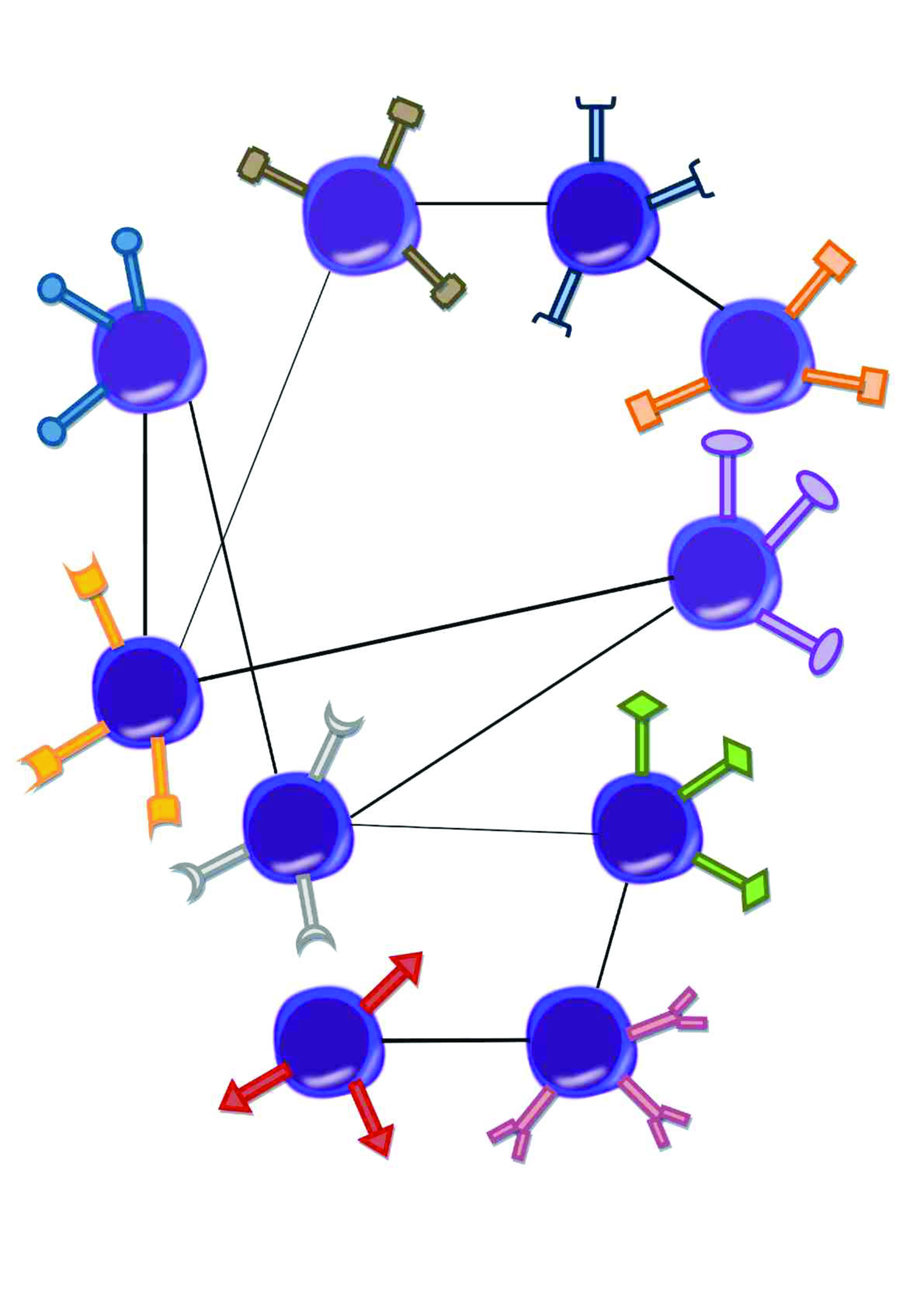
3.1 Graphs

The system of $N$ lymphocytes interacting pairwise with a coupling $J_{ij}$ can be envisaged by means of a graph $\mathcal{G}$, whose nodes represent lymphocytes and a link between them is drawn whenever the pertaining coupling is positive. Before proceeding, it is worth recalling that a generic graph $\mathcal{G}$ is mathematically specified by the pair $\{V,\Gamma\}$ consisting of a non-empty, countable set of points, $V$ joined pairwise by a set of links $\Gamma$. The cardinality of $V$ is given by $|V|=N$ representing the number of sites making up the graph, i.e. its volume. From an algebraic point of view, a graph $\mathcal{G}=\{V,\Gamma\}$ is completely described by its adjacency matrix $\mathbf{A}$: Every entry of this off-diagonal, symmetric matrix, corresponds to a pair of sites, and it equals one if and only if this couple is joined by a link, otherwise it is zero. The number of nearest-neighbors of the generic site $i$, referred to as coordination number or degree, can be recovered as a sum of adjacency matrix elements: $k_{i}=\sum_{j\in V}A_{ij}$.

In our model the graph describing the interaction among lymphocytes is a random graph where links are drawn with probability $p_{\alpha,L}$ which, in general, depends on the way strings $\xi$’s are extracted and on the the way affinity $f_{\alpha,L}$ is defined.

Here, due to the uniform distribution underlying the extraction of $\xi$’s, we have that the probability that $\xi_{i}^{\mu}$ and $\xi_{j}^{\mu}$ are complementary equals $1/2$ independently of $i,j$ and $\mu$. Therefore, the probability that they display $c_{ij}$ (hereafter simply $c$) complementary entries follows a binomial distribution which reads off as

$$\mathcal{P}(c)=\left(\frac{1}{2}\right)^{L}\binom{L}{c}.$$ (3.4)

Correspondingly, we have that lymphocytes $i$ and $j$ are connected together, namely that $f_{\alpha,L}(\xi_{i},\xi_{j})>0$, when $c_{ij}(\alpha+1)-L$ is positive (see Eq. 3.2) and this occurs with probability

$$p_{\alpha,L}=\sum_{c=\lfloor L/(\alpha+1)\rfloor+1}^{L}\mathcal{P}(c),$$ (3.5)

where $\lfloor x\rfloor=\max\{n\in N|n\leq x\}.$

The link probability $p_{\alpha,L}$ (see Eq. (3.5)) is, at least for large $L$, independent of the chosen couple, hence giving rise to an Erdös-Renyi graph $\mathcal{G}(N,p_{\alpha,L})$ [38] characterized by a binomial degree distribution

$$P(k)=\binom{N}{k}p_{\alpha,L}^{k}(1-p_{\alpha,L})^{k},$$ (3.6)

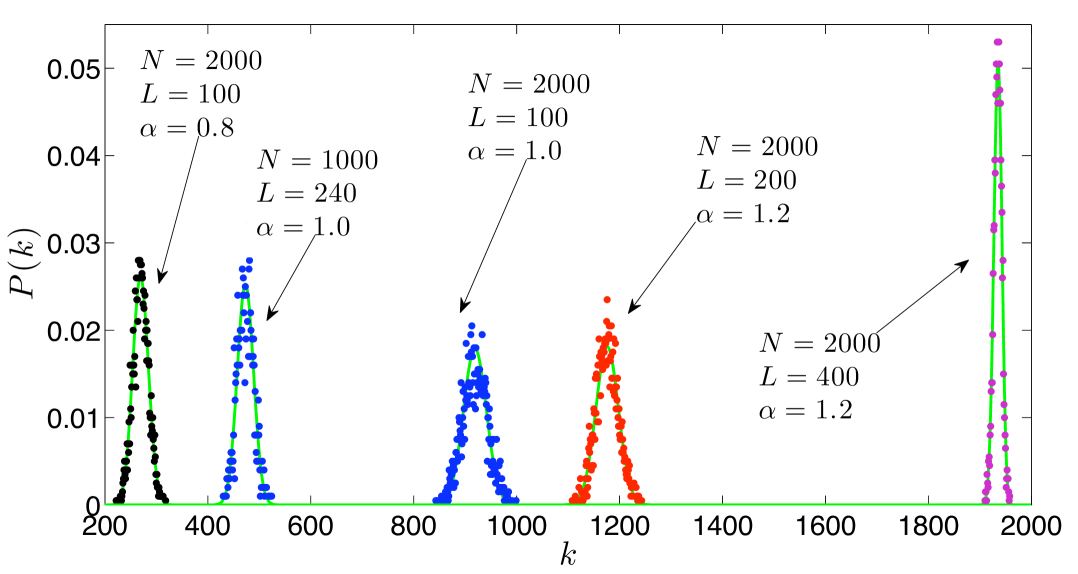
representing the probability that a generic node has $k$ nearest neighbors; the average degree follows as $\langle k\rangle=p_{\alpha,L}(N-1)$, or, more simply, for $N$ large, we use $\langle k\rangle=p_{\alpha,L}N$. In Fig. (3.2) we show the agreement between numerical data and analytic estimates (Eq. 3.6) for the degree distribution $P(k)$; different values of $N$, $L$, and $\alpha$ are considered. The good agreement among data corroborates the analytical derivation based on the lack of correlation among links.

Figure 3.2: Degree distribution $P(k)$ for different values of $N$, $L$ and $\alpha$; data from numerics ($\bullet$) and analytic estimates (green lines), see Eq. (3.6), are compared.

3.2 Dilution

The link probability $p_{\alpha,L}$ defined in Eq. (3.5) yields information about the dilution of the graph: the larger $p_{\alpha,L}$, the more connected the graph. For instance, at given $L$, the dilution of the graph can be controlled by properly tuning the parameter $\alpha$.

As well known, by increasing the link probability from $0$ upwards, the (infinite) Erdös-Renyi random graph undergoes a percolation transition; namely there exists a critical link probability $p_{c}$ such that when the link probability starts to get larger than $p_{c}$ a so called “giant component”, displaying a size $\mathcal{O}(N)$, i.e. infinite in the thermodynamic limit, suddenly appears [38].

Indeed, the Erdös-Renyi random graph $\mathcal{G}(N,p)$ can be obtained from the complete graph of $N$ vertices, $K_{N}$, by retaining each edge with probability $p$ and deleting it with probability $1-p$, independently of all other edges. Analogously, the topology of the idiotypic network we are introducing in this work can be recovered from $K_{N}$ by conserving and erasing links with probability $p_{\alpha,L}$ and $1-p_{\alpha,L}$, respectively.

The Molloy-Reed criterion for percolation [39] shows that, for this model, a giant component exists if and only if $p$ is larger than $1/N$. More precisely, setting $p=\langle k\rangle/N$, if we denote with $C_{1}$ the largest component in $\mathcal{G}(N,p)$ and with $|C_{1}|$ the cardinality of the set $C_{1}$, then we have the following results (see [40]): if $\langle k\rangle<1$, then with high probability (w.h.p.) $|C_{1}|\sim\log N$, if $\langle k\rangle>1$, then w.h.p. $|C_{1}|\sim N$, while if $\langle k\rangle=1$, the situation is more delicate and one can state $|C_{1}|\sim N^{2/3}$.

Therefore, it is important to analyze in more details the behavior of $p_{\alpha,L}$ as a function of $\alpha$ and $L$. For $\alpha=1$ it is straightforward to see that $p_{1,L}=1/2$, due to the symmetry of the distribution $\mathcal{P}(c)$ with respect to $c=L/2$ .

More generally, for large $L$ we can adopt a continuous description and write $p_{\alpha,L}$ (see Eq. (3.5)) as

$$p_{\alpha,L} \approx \int_{L/(\alpha+1)}^{L}\mathcal{P}(c)\,dc\approx\int_{L/(\alpha+1)}^{L}\sqrt{\frac{2}{\pi L}}\,e^{-\frac{(c-L/2)^{2}}{L/2}}\;dc$$ (3.7)

$$= \frac{1}{2}\left[\mathrm{Erf}\left(\sqrt{\frac{L}{2}}\right)-\mathrm{Erf}\left(\frac{(1-\alpha)}{(1+\alpha)}\sqrt{\frac{L}{2}}\right)\right],$$ (3.8)

where we replaced the distribution $\mathcal{P}(c)$ with the normal distribution, having mean $L/2$ and variance $L/4$; in fact, for $L$ large enough, the skew of the distribution $\mathcal{P}(c)$ is not too great and we can approximate the binomial distribution by the normal distribution [35]. From Eq. 3.7 we can calculate the derivative of $p_{\alpha,L}$ with respect to $\alpha$, which reads off as

$$\frac{\partial p_{\alpha,L}}{\partial\alpha}\approx\sqrt{\frac{2L}{\pi}}\frac{1}{(1+\alpha)^{2}}e^{-\frac{L}{2}\tilde{\alpha}^{2}},$$ (3.9)

where we called $\tilde{\alpha}\equiv(1-\alpha)/(1+\alpha)$.

We now turn to the coupling strength introduced in Eq. (3.3) and we notice that we can write $\tilde{J}_{ij}=\exp[c_{ij}(\alpha+1)-L]$, whenever $c_{ij}>L/(\alpha+1)$, otherwise $\tilde{J}_{ij}=0$. Hence, its mean value, averaged over all possible matchings between two binary strings, can be written as (see Eqs. (3.5),(3.3)):

$$\langle\tilde{J}\rangle_{\alpha,L} \approx \int_{L/(\alpha+1)}^{L}e^{c(\alpha+1)-L}\,\sqrt{\frac{2}{\pi L}}\,e^{-\frac{(c-L/2)^{2}}{L/2}}\,dc$$

$$= \frac{1}{2}e^{\frac{L}{8}(\alpha^{2}+6\alpha-3)}\left\{\mathrm{Erf}\left[\frac{\alpha^{2}+4\alpha-1}{2(1+\alpha)}\sqrt{\frac{L}{2}}\right]+\mathrm{Erf}\left[\frac{1-\alpha}{2}\sqrt{\frac{L}{2}}\right]\right\}$$

Now, we focus on the regime $L\gg 1$ and, according to the value of the (finite) parameter $\alpha$, we distinguish among the following cases:

• $\alpha=1$
  The expressions in Eqs. (3.8-3.2) can be evaluated exactly obtaining, respectively:

  $$p_{1,L}\approx\frac{1}{2}\mathrm{Erf}\left(\sqrt{\frac{L}{2}}\right)=\frac{1}{2}\left[1-\mathcal{O}\left(\frac{e^{-L/2}}{\sqrt{L}}\right)\right],$$ (3.11)

  $$\frac{\partial p_{\alpha,L}}{\partial\alpha}\bigg{|}_{\alpha=1}\approx\frac{1}{2}\sqrt{\frac{L}{2\pi}},$$ (3.12)

  and

  $$\langle\tilde{J}\rangle_{1,L}\approx\frac{1}{2}\;e^{\frac{L}{2}}\;\mathrm{Erf}\left(\sqrt{\frac{L}{2}}\right)=\frac{1}{2}e^{\frac{L}{2}}\left[1-\mathcal{O}\left(\frac{e^{-\frac{-L}{2}}}{\sqrt{L}}\right)\right]\approx e^{\frac{L}{2}}p_{\alpha,L}.$$ (3.13)

• $\alpha<1$
  

  $$p_{\alpha,L}\approx\sqrt{\frac{1}{2\pi L}}\;\frac{1}{\tilde{\alpha}}\;e^{-\frac{L}{2}{\tilde{\alpha}}^{2}}\left[1+\mathcal{O}\left(\frac{1}{L}\right)\right],$$ (3.14)

  hence, $p_{\alpha,L}\to 0$ as $L\to\infty$. Moreover, for $\alpha>-1+\sqrt{2}\approx 0.41$

  $$\langle\tilde{J}\rangle_{\alpha,L}\approx e^{\frac{L}{8}(\alpha^{2}+6\alpha-3)}\left[1-\mathcal{O}\left(\frac{e^{-\frac{L(1-\alpha)^{2}}{8}}}{\sqrt{L}}\right)\right],$$ (3.15)

  which is diverging for $\alpha>-3+2\sqrt{3}\approx 0.46$.

• $\alpha>1$
  

  $$p_{\alpha,L}\approx 1-\mathcal{O}\left(\frac{e^{-\frac{L}{2}\tilde{\alpha}^{2}}}{\sqrt{L}}\right),$$ (3.16)

  hence $p_{\alpha,L}\to 1$ as $L\to\infty$. Moreover, analogously to the previous case,

  $$\langle\tilde{J}\rangle_{\alpha,L}\approx e^{\frac{L}{8}(\alpha^{2}+6\alpha-3)}\left[1-\mathcal{O}\left(\frac{e^{-\frac{L(1-\alpha)^{2}}{8}}}{\sqrt{L}}\right)\right].$$ (3.17)

The asymptotic expressions above are all consistent with numerical results which indeed confirm the validity of the Gaussian approximation already for $L\sim 10^{2}$. Moreover, we notice that in the limit $L\rightarrow\infty$ the link probability $p_{1,L}$ is a step function with diverging derivative in $\alpha=1$ and $p_{\alpha,L}=1$ for $\alpha>1$, while $p_{\alpha,L}=0$ for $0\leq\alpha<1$. In Fig. (3.3) we show the behavior of $p_{\alpha,L}$ as $L$ and $\alpha$ are varied.

Figure 3.3: Link probability $p_{\alpha,L}$ for a system of $N=4000$ nodes as a function of $\alpha$ and of $L$.

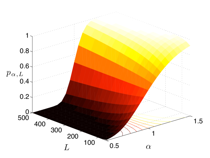
In order to characterize the dilution of the graph under study, a proper parameter is the average coordination number $\langle k\rangle=p_{\alpha,L}N$, as it represents the average number of links stemming from a node. In principle, $\langle k\rangle$ depends on $\alpha,L$ and $N$, which in our model cover a well precise physical and biological meaning. In fact, while $\alpha$ derives from the chemical-physical interactions arising among antibodies and antigens, and can be set independently of $N$ and $L$, the latter parameters $N$ and $L$ are intrinsically connected with each other. First of all, for strings of length $L$, the minimum number $N$ of agents has to be lower than $2^{L}$, if we want to avoid repetitions. Actually, as underlined in Sec. (2.2), $N$ is expected to be much smaller than $2^{L}$. Moreover, a proper scaling of the system size should preserve its (global) topological features, namely $\langle k\rangle$. In particular, $\langle k\rangle$ must be finite in order to have a well-defined thermodynamic limit for $N\to\infty$ [10, 36, 52]; all other cases would be either trivial ($\langle k\rangle\to 0$) or un-physical ($\langle k\rangle\to\infty$). Thus, on the one hand $\langle k\rangle$ specifies the degree of dilution of our idiotypic network, on the other hand it crucially affects the statistical mechanics of the whole system. Therefore, it is natural to describe a system by means of the three parameters $\alpha$, $L$ and $\langle k\rangle$. Then, the number of nodes $N$ follows as

$$N=\frac{\langle k\rangle}{p_{\alpha,L}}\approx\frac{2\langle k\rangle}{\mathrm{Erf}\left(\sqrt{\frac{L}{2}}\right)-\mathrm{Erf}\left(\tilde{\alpha}\sqrt{\frac{L}{2}}\right)},$$ (3.18)

where we used Eq. (3.8). In particular, for $\alpha<1$, one can write (see Eq. 3.14)

$$N\approx\sqrt{2\pi L}\;\langle k\rangle\tilde{\alpha}\;e^{\frac{L}{2}\tilde{\alpha}^{2}},$$ (3.19)

which should be compared with Eq. (2.2), to get $f(L)\sim\sqrt{L}$.

Figure 3.4: Left panel: Idiotypic network obtained for $\alpha=0.7$, $L=140$; for the sake of clarity we fixed a small number of nodes $N=30$. Right panel: Representation of the connectivities among a group of neonatal antibodies found by Varela and Coutinho in [28].

Finally, we notice that several independent experiments, lead on natural antibodies in neonatal mice, have evidenced that the network is highly connected: each idiotype is able to recognize on average $20-25\%$ of a given panel [68, 66, 67]. However, such connectivity decreases with time and it is expected to reach a steady state value, as corroborated by higher values of dilution in adult mice [72]; in particular, in [73] the connectivity in adult immune systems is estimated around $3-5\%$. Following these data, in our system, meant for a mature immune system, the link probability $p_{\alpha,L}$ is expected to be approximately $0.04$, which provides a first hint for selecting the region $\alpha<1$. Moreover, recalling $N\sim\mathcal{O}(10^{14})$, we consistently expect $\langle k\rangle\sim\mathcal{O}(10^{12})$. Therefore, in our model a realistic system may be obtained by fixing $\alpha=0.7$, $L=140$ and $\langle k\rangle\sim\mathcal{O}(10^{12})$, then from Eq. (3.7) we get $p_{\alpha,L}\approx 0.04$, from which we recover $N\sim\mathcal{O}(10^{14})$; the whole framework is therefore quantitatively consistent with real data.

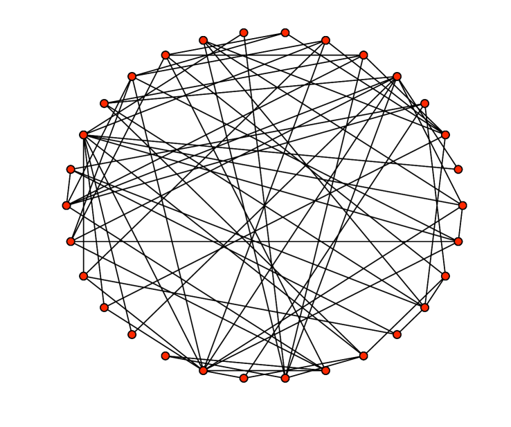
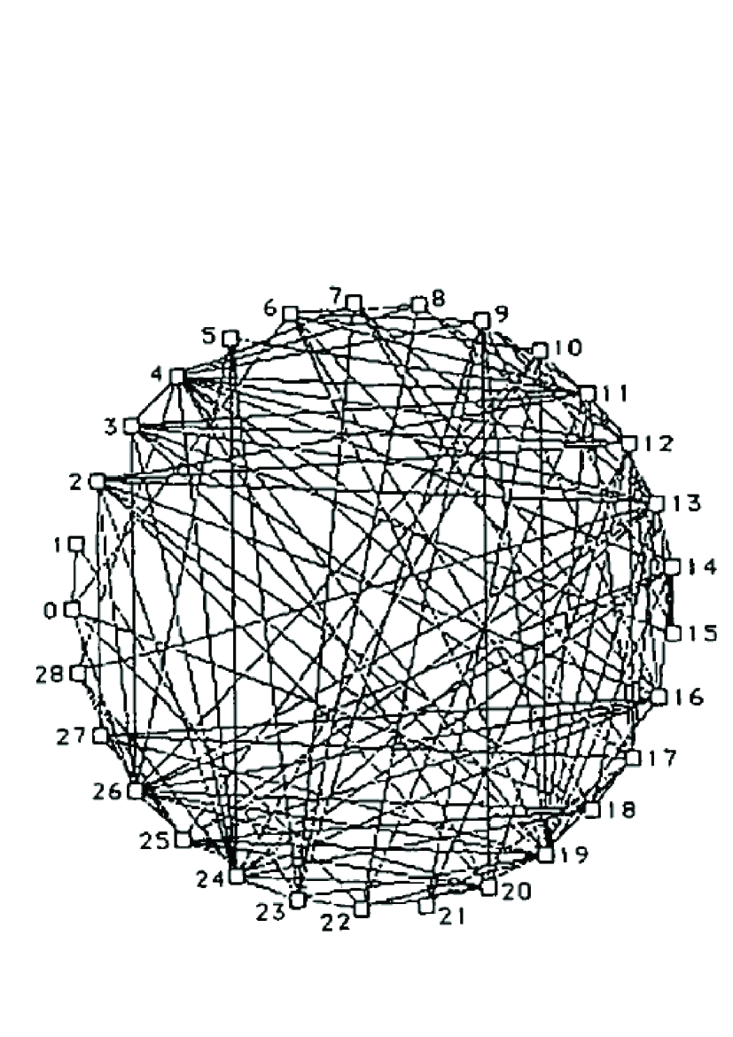
We conclude this section by showing a typical topological structure corresponding to parameters $\alpha=0.7$ and $L=80$, see Fig. 3.4, left panel; a comparison with the network obtained experimentally in [28], right panel, is also provided. The similarity between the two structures is manifest and suggests that the Erdös-Renyi topology which emerges from our minimal assumption is consistent with real data.

3.3 Weighted connectivity

In Sec. (3.1) we introduced the degree $k_{i}$ which represents the number of lymphocytes “in contact” with the lymphocyte labeled as $i$ and making up the set denoted as $V_{i}\subseteq V$. This means that the lymphocyte $i$, can interact with lymphocytes in $V_{i}$ through the pertaining antibodies described by the string $\xi_{i}$.

The coordination number has been shown to play a crucial role in the reactivity of antibodies [27]: the patterns of cross-reactivity between collections of idiotypes have been organized by experimental immunologists in matrices which are just the adjacency matrices describing the affinity among idiotypes. Such matrices have been revealed to be be arranged in blocks: a high-connectivity block (including nodes characterized by large degree), a “mirror block” (intermediate degree) and a low-connectivity block (small degree). These blocks were analyzed in their independent contributions through simulations by Varela et al. [27] who concluded that the larger the degree, the lower the reactivity of the corresponding lymphocytes and the greater their degree of tolerance. Hence the various groups play different roles: the mirror group accounts for intrinsic oscillations, while highly connected nodes may act as initial organizers of the immune system. In this framework, and according to the autopoietic view, autoimmunity arises not because of the presence of self-reactive clones, but because such clones are or become “not properly” connected to the network. As a result, self/non-self discrimination turns out to be an emergent property of the immune network which is therefore able to organize the mature repertoire. It follows naturally that establishing the structure of the immune system is a task of great importance as it would allow to figure out possible strategies to cope with autoimmune diseases.

In our model the adjacency matrix is actually weighted since links are endowed with a weight $J_{ij}$, which allows to introduce a weighted degree $w_{i}$ as

$$w_{i}(\alpha,L,\langle k\rangle)\equiv\sum_{j=1}^{N}J_{ij}(\alpha,L).$$ (3.20)

Notice that the local quantity $w_{i}$ provides finer information with respect to $k_{i}$, being directly connected with the "internal" stimulus felt by lymphocyte $i$: recalling the Hamiltonian of Eq. (2.6), and assuming, for the sake of simplicity, the zero noise limit so that all lymphocyte in $V_{i}$ are quiescent ($m_{j}=-1,\forall j\in V_{i}$), the local field acting on $i$ is just $\varphi_{i}=-\sum_{j=1}^{N}J_{ij}m_{j}=w_{i}$.

For a given system $(\alpha,L,\langle k\rangle)$ the average weighted degree can be calculated as

$$\langle w\rangle_{\alpha,L,\langle k\rangle}=\sum_{k}P(k)\sum_{c_{1},c_{2},...,c_{k}=L/(\alpha+1)}^{L}\prod_{i=1}^{k}\mathcal{P}(c_{i})\sum_{i=1}^{k}\frac{e^{c_{i}(\alpha+1)-L}}{\sum_{c_{i}}\mathcal{P}(c_{i})e^{c_{i}(\alpha+1)-L}}.$$ (3.21)

Actually, it is convenient to introduce the "quenched averages" $\bar{J}(\alpha,L)$ and $\bar{w}(\alpha,L,\langle k\rangle)$, obtained by averaging the couplings $J_{ij}$ and the weighted degree $w_{i}$ over all links and nodes, respectively, of a given realization, namley

$$\bar{J}=\frac{\sum_{i=1}^{N}\sum_{j=1}^{N}J_{ij}}{N(N-1)}=\bar{J},$$ (3.22)

and

$$\bar{w}=\frac{\sum_{i=1}^{N}w_{i}}{N}=\frac{\sum_{i=1}^{N}\sum_{j=1}^{N}J_{ij}}{N}=(N-1)\bar{J}.$$ (3.23)

Now, for large $N$ and $L$ the "quenched averages" $\bar{J}(\alpha,L)$ and $\bar{w}(\alpha,L,\langle k\rangle)$ converge to the "ensemble averages" $\langle J\rangle_{\alpha,L}$, that is $\langle w\rangle_{\alpha,L,\langle k\rangle}\approx(N-1)\langle J\rangle_{\alpha,L}$ and, being that $\langle J\rangle_{\alpha,L}$ equals one by definition, we have that $\langle w\rangle_{\alpha,L,\langle k\rangle}$ scales linearly with $N$. Analogously, due to the uncorrelatedness among $J_{ij}$’s, one can use Bienayme prescription and write

$$\mathrm{Var}(w_{i})=\mathrm{Var}\left(\sum_{j=1}^{N}J_{ij}\right)=\sum_{j=1}^{N}\mathrm{Var}(J_{ij})=N\mathrm{Var}(J_{ij})$$ (3.24)

where $\mathrm{Var}(x)\equiv\bar{x^{2}}-\bar{x}^{2}\equiv\sigma_{x}^{2}$ is the variance of the variable $x$, that is the expected value of the square of the deviation of $x$ from its own mean $\bar{x}$. Now, the variance for $J_{ij}$ can be estimated via Eq. (3.3) and Eq.(3.4)

$$\langle J^{2}\rangle_{\alpha,L} = \frac{1}{\langle\tilde{J}\rangle_{\alpha,L}^{2}}\int_{\frac{L}{\alpha+1}}^{L}\exp{\left[2c(\alpha+1)-2L\right]}\sqrt{\frac{2}{\pi L}}e^{-\frac{(c-L/2)^{2}}{L/2}}\;dc$$

$$= \frac{e^{\frac{L}{2}(\alpha^{2}+4\alpha-1)}}{2\langle\tilde{J}\rangle_{\alpha,L}^{2}}\left[\mathrm{Erf}\left(\frac{\alpha(3+\alpha)}{1+\alpha}\sqrt{\frac{L}{2}}\right)-\mathrm{Erf}\left(\alpha\sqrt{\frac{L}{2}}\right)\right].$$

Now, with some algebra and recalling Eq. (3.2), we get the following estimate

$$\langle J^{2}\rangle_{\alpha,L} \approx 2e^{\frac{L}{4}(\alpha+1)^{2}}$$ (3.25)

$$\times\frac{\left[\mathrm{Erf}\left(\frac{\alpha(3+\alpha)}{1+\alpha}\sqrt{\frac{L}{2}}\right)-\mathrm{Erf}\left(\alpha\sqrt{\frac{L}{2}}\right)\right]}{\left[\mathrm{Erf}\left(\frac{\alpha^{2}+4\alpha-1}{2(1+\alpha)}\sqrt{\frac{L}{2}}\right)+\mathrm{Erf}\left(\frac{1-\alpha}{2}\sqrt{\frac{L}{2}}\right)\right]^{2}}$$

$$= \frac{1}{2}e^{\frac{L}{4}(-\alpha^{2}+2\alpha+1)}\frac{1}{\alpha\;\sqrt{2\pi L}}\left[1-\mathcal{O}\left(\frac{1}{L}\right)\right].$$ (3.26)

After noticing that, for $1-\sqrt{2}<\alpha<1+\sqrt{2}$ the exponent is positive, yielding $\langle J^{2}\rangle_{\alpha,L}\gg\langle J\rangle_{\alpha,L}^{2}=1$, we can write the standard deviation for the coupling strength as

$$\sigma^{J}_{\alpha,L}\approx\sqrt{\langle J^{2}\rangle_{\alpha,L}}\sim\frac{1}{\sqrt[4]{L}}e^{\frac{L}{8}(-\alpha^{2}+2\alpha+1)}.$$ (3.27)

Moreover, one can write

$$\sigma^{w}_{\alpha,L}\approx\sqrt{N\langle J^{2}\rangle_{\alpha,L}}\approx\sqrt[4]{L}\;e^{\frac{L}{4}\frac{(-2a^{4}+9a^{2}+6a+3)}{(1+a)^{2}}},$$ (3.28)

where in the last expression we used Eq. (3.19).

Figure 3.5: Standard deviation $\sigma^{J}_{\alpha,L}$ as a function of the system size $N$; the parameter $L$ is properly rescaled in order to keep $\langle k\rangle$ fixed and equal to $60$ (red) or to $100$ (black); different symbols represent different choises for $\alpha$, as shown by the legend. The straight line represents the first bisector.

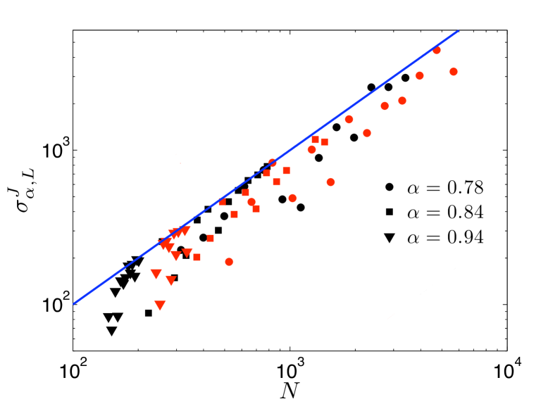
In Fig. (3.5) we show, as a function of $N$ and for several choices of $\alpha$, the standard deviation $\sigma^{J}_{\alpha,L}$; notice that while $N$ is varied, $L$ is properly scaled in order to keep $\langle k\rangle$ fixed. The log-log scale plot highlights a regime, for large enough $N$, where a power law growth for $\sigma^{J}_{\alpha,L}$ holds.

3.4 Circuits

In this section we want to analyze the number and the relative weight of small loops present in the random graph $\mathcal{G}(N,p_{\alpha,L})$, previously introduced to describe the idiotypic network. This kind of information allows not only to deepen the topological description of the immune network, but it will also be useful in the following sections when studying the system response to external stimuli.

In fact, we recall that due to the lacking of a perfect match among antibodies, a given lymphocyte, say $\sigma_{1}$, undergoing clonal expansion, may elicit one (or more) of the best Jerne counterparts (even spurious state may respond), say $\sigma_{2}$. The latter undergoing clonal expansion too, may elicit another lymphocyte among the best Jerne spurious state, say $\sigma_{3}$, and so on. Now, since $\sigma_{1}$ and $\sigma_{3}$ both have large affinity, i.e. complementarity, with the same state $\sigma_{2}$, they are expected to be similar. Analogously, $\sigma_{4}$ is expected to be similar to $\sigma_{2}$ and therefore to disply a large affinity with both $\sigma_{1}$ and $\sigma_{3}$. As a result, such loops built by four lymphocytes which are mutually Jerne states are expected to be more stable than the loops built by three lymphocytes.
Of course, again due to the multi-attachment (able to generate spurious states) the information gets lost when increasing the size of the loop such that large loops are unexpected; in the following particular attention will be paid to loops of length $3$ and $4$.

Let us now formalize and analyze mathematically the problem. First of all, we define a circuit of length $l$ as the edge set $\ell_{l}$ of an undirected closed path without repeated edges, that is $\ell_{l}=\{(i_{1},i_{2}),(i_{2},i_{3}),...,(i_{l},i_{1})\},$ with $(i_{k},i_{\mathrm{mod}(k+1,l)})\in\Gamma$, for any $k\in[1,l]$.

Then, we denote with $n_{l}$ the number of circuits of length $l$ present in the graph; it’s worth recalling that $n_{l}$ is a purely topological quantity depending only on the adjacency matrix $\mathbf{A}$. Now, the number of possible circuits reads as $\frac{1}{2l}\frac{N!}{(N-l)!}$, in fact, choosing such a circuit implies to select an ordered list of $l$ vertices, modulo the orientation and the starting point of the path. Now, for an Erdös-Renyi random graph the probability for a circuit to be effectively present in the network only depends on its length, being given by the link probability to power $l$; in particular, here we get

$$n_{l}=\frac{1}{2l}\frac{N!}{(N-l)!}p_{\alpha,L}^{l}.$$ (3.29)

For short cycles with $l\ll N$, we can approximate the previous expression as

$$n_{l}\approx\frac{1}{2l}\langle k\rangle^{l},$$

where we used that the average degree in $\mathcal{G}$ is $\langle k\rangle=p_{\alpha,L}(N-1)$. Therefore, above the percolation threshold, the number of circuits grows exponentially fast with their length.

It is also possible to calculate the number of circuits of length $l$, such that they include a node of degree $k$; this is simply given by

$$n_{l}(k)=\frac{1}{2l}\frac{(N-3)!}{(N-l)!}p^{l-2}k(k-1)\approx\frac{k^{2}}{2lN}\langle k\rangle^{l-2},$$ (3.30)

where the last expression holds for $l$ small and $k$ large. As a consequence, as $l$ is increased, the number of circuits increases exponentially and the rate of growth increases with $k$.

As underlined before, our network can not be described in a purely topological way, i.e. in terms of the adjacency matrix only, as the coupling strength associated to each link has an important physical meaning. Consequently, circuits should also be measured according to the couplings $J_{ij}$, or weights $w_{i}$, of the pertaining links or sites, respectively: the overall strength $J_{\ell_{l}}$ associated to the circuit denoted as $\ell_{l}=\{(i_{1},i_{2}),(i_{2},i_{3}),...,(i_{l},i_{1})\}$, is therefore given by

$$J_{\ell_{l}}=\frac{1}{l}\sum_{k=1}^{l}J_{i_{k},i_{k+1}},$$ (3.31)

being $i_{l+1}\equiv i_{1}$, while the overall weight is

$$w_{\ell_{l}}=\frac{1}{l}\sum_{k=1}^{l}w_{i_{k}}.$$ (3.32)

Notice that $J_{\ell_{l}}$ represents the intrinsic robustness of the circuit $\ell_{l}$, while $w_{\ell_{l}}$ represents the overall (relative) influence from the external environment to the circuit $\ell_{l}$. In the following we highlight the role of the quantities $J_{\ell_{l}}$ and of $w_{\ell_{l}}$, by considering a special situation.

Let us assume, for the sake of simplicity, that we are in the zero noise limit, so to discard the $\beta$ dependence of the quiescent state. In this condition, and in the absence of external stimuli we have $m_{k}=-1,\forall k\in V$. Now, when a sufficiently high concentration of the antigen $\bar{\xi}_{i}$ is introduced, the $i$th clone will undergo a clonal expansion, so that $m_{i}>-1$.

Then, the stimulus can spread from $i$ to nodes in $V_{i}$ and so on throughout the network in a cascade fashion, possibly coming back to $i$, hence providing a reinforcement feedback. In this case we say that a “firing circuit" has established. Given a circuit $\ell_{l}$ we say that it is firing if $m_{i_{k}}>-1$, for any $k\in[1,l]$. The magnitude of the firing circuit can be measured in terms of global firing concentrations, namely $\sum_{k=1}^{l}c_{i_{k}}/l\in[1,M]$, see Eq. (2.4).

Due to self-reinforcement, a firing circuit can survive even when the external stimulus has expired; the long-time persistence of a firing circuit can be estimated by means of the ratio $J_{\ell}/w_{\ell}$: the larger the ratio, the more important the self-reinforcement with respect to the neighborhood (possibly non-firing) and therefore the more likely the persistence. Interestingly, the persistence of firing circuits yields storage memory of previous infection, hence, finding the conditions for their establishment can be very important.

Figure 3.6: Distributions for overall strength $J_{\ell}$ (upper panel) and overall weight (lower panel) concerning circuits of length $l=3$ (triangles) and $l=4$ (squares). We also distinguished between circuits passing through lowly-conned nodes (Non-self, represented in red and in pink) and through highly-connected nodes (Self, represented in blue and in green), as shown by the legend. From the upper panel it is clear that for $l=4$ the overall strength is larger than for $l=3$. The graph considered is made up of $N=500$ nodes, moreover $\alpha=0.74$ and $L=80$.

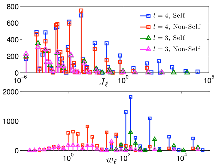
In this context we are interested in short circuits rather than long $\mathcal{O}(N)$ ones, the latter evidently require more strict conditions for their establishment and should actually be avoided as they would correspond to a broad response involving most lymphocytes, including those directed against self. In particular, we focus the attention on circuits of length $l=3$ and $l=4$, which are expected to result in sensitively different overall strengths $J_{\ell}$. In fact, the former corresponds to a frustrated configuration giving rise to a relatively small overall strength. More precisely, since links derive from a large degree of complementarity between the two adjacent nodes, circuits of odd, small length must display at least one weak edge; on the other hand, when the length is even this kind of frustration can be avoided.

As for the overall weight $w_{\ell}$, its value strongly depends on whether the circuit contains a highly-connected node, namely a node belonging to the left-hand side of the distribution $P(w)$; indeed, as we will see in the following section, such nodes are typically connected with analogously highly-connected nodes.

In Fig. 3.6 we show the distributions obtained for $J_{\ell}$ (upper panel) and for $w_{\ell}$ (lower panel), when considering all the circuits passing through lowly-connected and highly-connected nodes respectively; both cases $l=3$ and $l=4$ are considered. From the data depicted in the figure we calculated the average overall strength which, for $l=4$ turns out to be more than twice the one pertaining to $l=3$; the former is larger than $1$, the latter is smaller than $1$ (we recall that $1$ is the expected coupling strength). In fact, as anticipated, a lymphocyte $\sigma_{1}$ and its corresponding anti-lymphocyte are unlikely to have a strong common neighbour. We also notice that the presence of a highly connected node within the circuit has dramatic effects on the distribution for $w_{\ell}$ which results to be shifted towards larger values; this means that circuits involving self-addressed nodes (i.e. those with high connectivity, vide infra) are also more unlikely to be elicited.

Chapter 4 Features of the model

4.1 Self/Non-Self recognition

Let us consider again the whole idyotipic network made of $N$ different clones, each characterized by a specific string of $L$ idyotopes; once $\alpha$ is fixed, the affinity between two different nodes is specified by Eq. (3.2) from which the coupling in Eq. (3.3) follows.

Before turning to the analysis of the distribution $P(w)$ and showing how it naturally allows to distinguish between self and non-self addressed antibodies, it is worth recalling the famous experiment lead by Stewart, Varela and Coutinho [27, 28]: they measured the affinity of a collection of antibodies and analyzed the related affinity matrices finding that these matrices are organized in blocks. More precisely, they distinguished a high-affinity block, two blocks of groups which are mirror of each other, and a low affinity remnant; then they showed that various groups play different roles: the mirror groups provide their model with various oscillations periods, while highly connected nodes maintain a “basic network background level" and may be looked at as self-addressed antibodies. Indeed, their large connectivity prevents them from readily react to a stimulus. This point of view is extremely interesting as it outlines a natural interpretation of the topological properties of the immune network. Not only, from an autopoietic point of view, it also sheds light on autoimmunity diseases: their origin would therefore lay on the “inadequate connection” of self-reactive clones.

Let us now consider the idiotypic network introduced in the previous section: with respect to the model introduced by Coutinho and Varela [28], here each link stemming from a given node $i$ has its own weight, which measures how strong the affinity between the relevant antibodies is, in such a way that, the information carried by $w_{i}$ is much reacher than the one carries by $k_{i}$. Hence, we will follow the experiment by Stewart, Varela and Coutinho [27, 28] by looking not at the degree distribution $P(k)$, but rather at the distribution $P(w)$.

We considered different systems $(\alpha,L,\langle k\rangle)$ and by numerical analysis we derived the distribution $P(w)$, which, on a semilogaritmic scale, can be properly fitted by a Gaussian distribution; the relevant best fits are represented by the green curves in Fig. 4.1. Such distributions naturally outline three main groups characterized by high (right-hand-side tail), intermediate (central region) and low (left-hand-side tail) weighted degree, respectively. Hence, recalling that a large weight implies a low reactiveness (see previous section), lymphocytes displaying low and high weighted degree can be labelled as non-self and self addressed lymphocytes, respectively. It is important to notice that, since the distribution $P(w)$ covers several orders of magnitude, the former will easily react even by low dose of nearest-neighbors (or antigens) (implicitly defining the low dose tolerance), while, for larger $w$, the ability to react decreases progressively, up to prohibitive values of antigenic concentration.

Now, starting from $P(w)$ we want to focus on couples of Ig and anti-Ig and figure out possible correlations in their weighted degrees. We first select non-self addressed lymphocytes, namely modes in the network corresponding to the left-hand side of the weighted degree distribution, and we look for their most tightly connected neighbors among the remaining $N-1$. This way, we distinguish couples $(i,\bar{i})$, where $i$ should be meant as a lymphocyte producing Ig directed against non-self agents and $\bar{i}$ as a lymphocyte producing so called anti-Ig able to respond to a significant growth in Ig’s concentration, according to Jerne’s idea of idiotypic network.

Figure 4.1: Weighted connectivity distributions (green line) for systems made up of $N=4000$ lymphocytes characterized by idiotypic strings of length $L=120$ and $\alpha=0.74$ (panel a), $L=120$ and $\alpha=0.82$ (panel b), $L=100$ and $\alpha=0.78$ (panel c,d); the average connectivity $\langle k\rangle$ gets $240$, $630$ and $290$, respectively. In blue we show the distribution of low-connected clones (panels $a$, $b$ and $c$) or high-connected clones (panel $d$) chosen and in red the distribution of the pertaining "anti-clones". Notice the semilogarithmic scale plot. The insets show the relevant matching $c_{ij}$ among all the couples Ig and anti-Ig detected in the whole system.

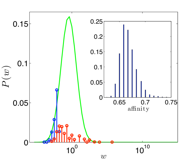
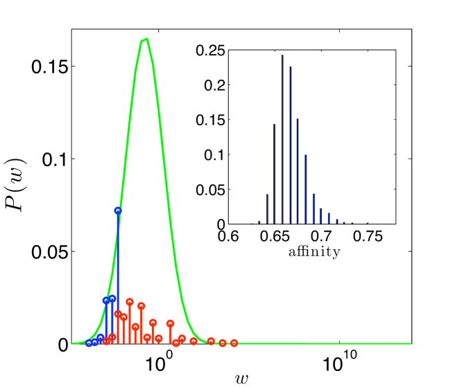
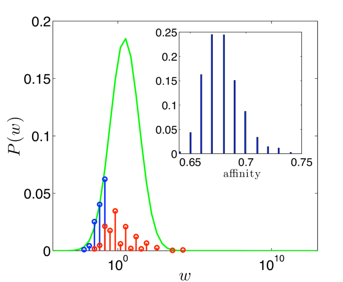
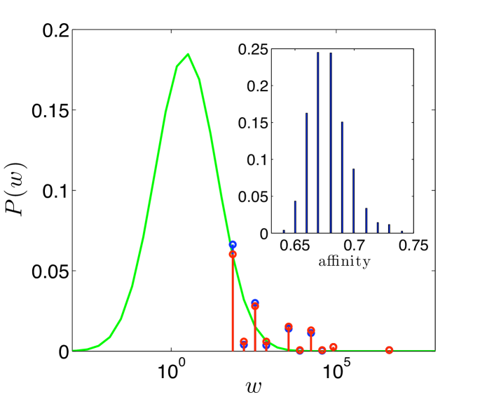
As shown in Fig. (4.1), when $i$ belongs to the low weighted-degree region, the corresponding $\bar{i}$ typically falls in the intermediate region of the distribution, hence fitting the “mirror block”; this holds for several choices of $\alpha$, $L$ and $\langle k\rangle$ (see panels $a$, $b$ and $c$).

Let us now turn to the right-hand side of the weighted-degree distribution and, analogously, we distinguish couples $(j,\bar{j})$, where $j$ represents a lymphocyte producing Ig directed against self agents and $\bar{j}$ as the relevant anti-Ig able (see panel $d$). In this case anti-Ig still belongs to the highly-connected group, that is they should as well be meant as directed to self-agents. This result is easy to see: Since by definition $j$ exhibits a large weight $w_{j}$, it follows that, typically, $J_{j\bar{j}}\sim w_{j}$ as the main contribution to $w_{j}$ comes from $J_{j\bar{j}}$ and, analogously, $J_{j\bar{j}}\sim w_{\bar{j}}$. Otherwise stated, when a highly connected node is selected, there exists a correlation between $w_{j}$ and $w_{\bar{j}}$; on the other hand when a lowly connected node is considered, the contribution of $J_{i\bar{i}}$ to $w_{i}$ and to $w_{\bar{i}}$, respectively, is small enough not to bias $w_{\bar{i}}$. The very origin of such a different behavior of self and non-self anti-Ig lays in the wide range spanned by $w$.

As deepened in the following, anti-Ig’s play a crucial role in the establishment of memory effects, so that the “mirror block” here acquires the fundamental function of memory storage. Interestingly, such a memory storage here turns out to be effectively managed since it is restricted to non-self directed Ig only. Conversely, self directed Ig and relevant anti-Ig both set up the highly-connected group.

Another point worth being underlined concerns the affinity between Ig and anti-Ig; the affinity can be evaluated from the number of matchings $c_{ij}$, whose distribution is represented in the insets of Fig. (4.1): due to the uniform distribution underlying the extraction of $\xi$’s, the relative matching $c_{ij}/L$ resulting from all possible pairs is distributed around the value $1/2$ with a standard deviation scaling as $1/\sqrt{L}$. Hence, the expected affinity for Ig and anti-Ig can be estimated as $1/2(1+3/\sqrt{L})$. Recalling that in our model each entry in $\xi$ represents an epitope and that each Ig displays $\mathcal{O}(10^{2})$ epitopes, we have that the relative matching between Ig and anti-Ig falls in between $0.6$ and $0.7$. It is interesting to stress that experimental values are bounded by $0.6$ (and in general larger): This can be understood by analyzing a $l=4$ Jerne loop and measuring the binding ability of the last antibody Ab4 with the first Ab1. On average $>60\%$ of Ab4 molecules are able to link Ab1 [48].

The consistency among such data confirms the plausibility of interpreting $\xi$ as a string of $\mathcal{O}(10^{2})$ epitopes (even thought improvements in the binding percentage should be achieved by using more complex epitope distribution probabilities). Also, the relative small affinity found experimentally among most-tightly nodes corroborates the fact that the system is far from complete, namely that $N\ll 2^{L}$, consistently with the assumption of Eq. (2.2).

4.2 Low-dose tolerance

In this section we want to investigate the effects elicited by a concentration $c$ of a given antigen. Let us consider the antigen with specificity $\xi_{h^{i}}\equiv\bar{\xi_{i}}$, namely displaying perfect match with antibody $\xi_{i}$. The presence of a concentration $c$ of the antigen can be incorporated within the Hamiltonian $H$ describing the system by introducing an external field $\mathbf{h^{i}}$, whose element $h^{i}_{k}$ represents the coupling with the $k$-th antibody, namely

$$h^{i}_{k}=\exp{[f_{\alpha,L}(\xi_{k},\xi_{h^{i}})]}\Theta(f_{\alpha,L}(\xi_{k},\xi_{h^{i}})).$$ (4.1)

Indeed, the coupling strength between antigen and antibody is calculated according to the rule introduced in Chapter 3 for antibody-antibody interaction since the forces underlying the couplings are of the same nature. Therefore we can rewrite the Hamiltonian $(2.7)$ as

$$H(\sigma,\mathbf{J},\mathbf{h})=-\frac{1}{N}\sum_{k<j}^{N,N}J_{kj}m_{k}m_{j}+\sum_{k=1}^{N}c\;h^{i}_{k}m_{k},$$ (4.2)

where $c$ can be possibly tuned to mimic variations in the antigen concentration. This way, an arbitrary lymphocyte $k$ is subject to two stimuli, one deriving from the presence of the antigen, and the other from the presence of the remaining lymphocytes. This can be formalized by saying that the field acting on the $k^{th}$ node is

$$H_{k}=-\frac{1}{N}\sum_{j=1}^{N}J_{kj}m_{j}+c\;h^{i}_{k}.$$ (4.3)

In the absence of any antigen it is reasonable to consider all lymphocytes in a quiescent state, i.e. $m_{k}=-1$ (under the assumption of negligible noise) for any $k$; this provides the initial state assumed to be stationary when no antigen is at work. Hence, as the field $\mathbf{h^{i}}$ is switched on, we have

$$H_{k}=\frac{1}{N}w_{k}-c\;h^{i}_{k},$$ (4.4)

where we used Eq. (3.20). Now, if $H_{k}$ occurs to be negative, the state for the $k^{th}$ lymphocyte which minimizes the energy is the firing one, namely $m_{k}=+1$. Hence, assuming that all lymphocytes are quiescent, the condition for lymphocyte $k$ to fire is

$$c\;h^{i}_{k}>\frac{w_{k}}{N}.$$ (4.5)

This means that the minimal concentration necessary in order to elicit an immune response by $k$ is directly proportional to its degree $w_{k}$ and inversely proportional to its coupling $h^{i}_{k}$. This also suggests that, in the presence of the antigen $\xi_{h^{i}}$, the most reactive idiotype is not necessarily $\xi_{i}$, but rather it may be a spurious one which exhibits the lowest ratio $\frac{w_{k}}{h^{i}_{k}}$. Interestingly, the threshold mechanism determined by Eq. (4.5) consistently mimics the low-dose tolerance phenomenon: The immune system attacks antigens or, more generally proteins, if their concentrations is larger than a minimum value, which depends on the particular protein.

Implicitly this mechanism suggests possible interpretation even of the high dose tolerance: as what elicits a given lymphocyte is the product of the weighted connectivity with another agent (antigen or internal molecules) times its concentration (properly expressed via a magnetization function), it can not distinguish among self or antigen in an high dose.
Responding to high dose of antigen should, in principle, allow a response even to the self, whose defence turns out to be a primarily goal.
These analytical estimates have been checked by means of numerical simulations: For a given system $(\alpha,L,\langle k\rangle)$ we run several experiments, each for a different applied field $\xi_{h^{i}}$, where the concentration of the antigen is tuned from $0$ up to the minimal value $\tilde{c}^{i}$ necessary to elicit an immune response; data are reported in Fig. (4.2). On the $x$-axis we set the weighted degree of the first reactive lymphocyte and on the $y$-axis we set the minimal concentration $\tilde{c}$ of the agent $\xi_{h^{i}}$ able to give rise to an immune response, multiplied by $h^{i}_{i}=\exp(\alpha L)$; a linear dependence between $w$ and $\tilde{c}$ is evidenced by the fit, in agreement with Eq. (4.5). We therefore recover the important result from Varela et al [27, 28] that the reactivity of an antibody is closely related to its degree, where, here, the degree is more specifically meant as weighted degree.

Figure 4.2: Threshold concentration $\tilde{c}$ of antigen $\xi_{h^{i}}$ as a function of the weighted connectivity $w_{i}$ of the first reactive family, in systems with parameters $N=1000$, $\alpha=0.84$, $\langle k\rangle\approx 150$ (triangles) and $N=3000$, $\alpha=0.74$, $\langle k\rangle\approx 40$ (circles), respectively; for both cases we used $M=100$ and $L=140$. The level of noise is set as $\beta=1.0$, far above the critical value.

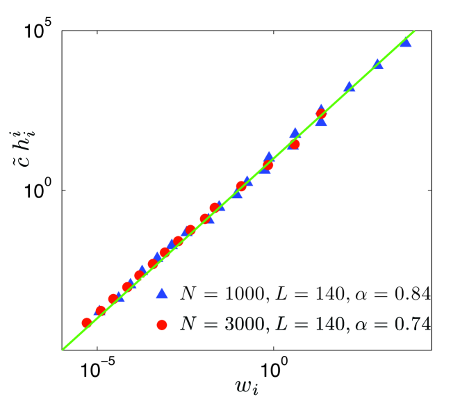
The linear scale between $\tilde{c}$ and $w$ has some significant consequences: The tolerated concentration of antigen directly reflects the (weighted) inhomogeneity of the graph. Otherwise stated, if the weighted degree spans a range, say, $\mathcal{O}(10^{k})$, the tolerated concentrations relevant to all lymphocytes making up the system is expected to span an analogously wide range. Hence, recalling that non-self-addressed Ig’s belong to the left tail of the weighted-degree distribution, while self-addressed Ig’s lay on the right tail, we have that the doses typically tolerated by the former are $k$ order of magnitude less that those tolerated by the latter. Now, as shown in Sec. 3.3, the weighted-degree distribution $P(w)$ exhibits a standard deviation scaling exponentially with $L$ or, analogously, algebraically with $N$, being $1/2$ a lower bound for the exponent. As a consequence, we expect that the region spanned by $w$ grows non-slower that $\sqrt{N}$; this means that for real systems the difference between doses tolerated by self and non-self is at least $\mathcal{O}(10^{7})$.

We finally stress that the low-dose tolerance emerges as a genuine collective effect directly related to the properties of the idyotopic network and, in particular, on the distribution of the weighted degree.

4.3 Multiple responses and spurious states

As explained in Sec. 4.2, the introduction of a concentration $c$ of a given antigen described by the external field $\mathbf{h^{i}}$ is able to increase the magnetization (concentration) of the node (lymphocyte) $i$, provided that $c$ is sufficiently high. In general, if the concentration is large enough, several clones, different from $i$, may prompt a response: some of them, say $j_{1},...,j_{p}$, (hereafter called spurious, once again in order to stress similarities with neural networks [9]) respond because of a non-null, though small, coupling with the external field, some others, say $j^{\prime}_{1},...,j^{\prime}_{p}$, (hereafter Jerne states for consistency) respond because they display a strong interaction $J_{ij}$ with the formers or with the specific Ig $i$. Spurious states can be very numerous according to the particular antigen considered and to its concentration; under proper conditions the response of spurious states can be even more intensive than the specific response from $i$. In fact, the reactivity of a given node $j$ is determined not only by the relevant antigenic stimulus $h^{i}_{j}$, but also by its local environment, namely by the concentration of firing lymphocytes to which $j$ is connected.

While in a neural networks framework spurious states correspond to "errors" during the retrieval (once a stimulus is presented) and should be avoided, in immune network spurious states are fundamental for an effective functioning of the whole machinery. In fact, when an antigen is introduced in the body, all the set of responders (proper lymphocyte and spurious states) do contribute to attack the enemy and neutralize it. Moreover, the reaction of spurious states can in turn have important consequences on the generation of memory cells and on the effectiveness of the secondary response. Accordingly, one can investigate whether it is possible to figure out proper strategies which can limit or increase the number the number of such spurious states. In particular, how the connectivity of the structure and the coupling patters $h^{i}_{k}$ influence this?

Here, we just want to analyze the overall response of the system outlining which kind of clone does react, that is, we distinguish between spurious states and Jerne states, i.e. anti-Ig. Results for different realizations of a system $(\alpha,L,\langle k\rangle)$ where the antigenic concentrations is set as $c\sim 10^{2}\tilde{c}$ are shown in Fig. (4.3); different symbols are used for spurious states (triangles) and for Jerne states (cirlces). For such concentrations the number of reactive spurious states is approximately twice the number of reactive Jerne states and a clear correlation between their weighted connectivity and $J_{j^{\prime}i,j}$ (Jerne state) can also be evidenced. Interestingly, Jerne states require a larger stimulus to react and this is due to the fact that the reaction is not directed, but rather mediated by the specific Ig $i$ or by a spurios state $j$.

Figure 4.3: Analysis of spurious states for different realizations of a system made up of $N=1000$ families and $M=10$ clones per family; we assumed $\alpha=0.84$ and $L=140$. Left panel: Field coupling $h^{i}_{j}$ (for reactive spurious states (triangles)) and interaction strength $J_{ij}$ (for reactive anti-antibodies (circles)) as a function of their weighted connectivity; each realization is depicted in a different color. Right panel: Schematic representation of connections between reactive antibodies.

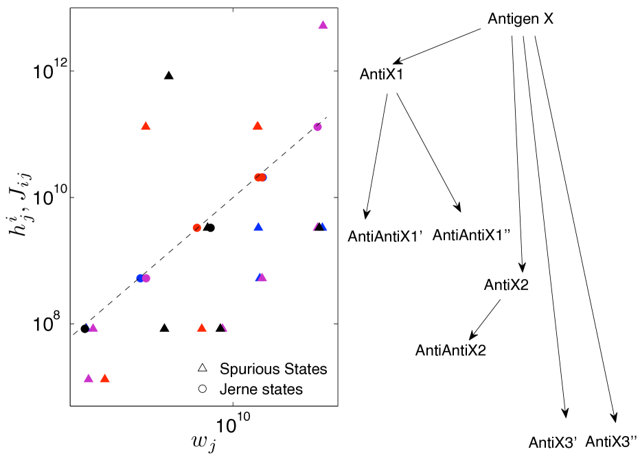
Furthermore it is also important to stress that apparently, without the introduction of spurious states, the amount of antibodies is greater than the amount of lymphocytes and this would be in conflict with the first postulate of immunology: consistency is obtained thanks to the lack of a perfect match among antibodies (or antibody and antigen), which allows multiple attachments ultimately accounting for a large over-counting of different responses.

4.4 Dynamical Memory

As well known, the immune system is able to develop memory effects; for this to happen the mutual interaction among lymphocytes is crucial. The activation of a lymphocyte $i$ must therefore be followed by the activation of the relevant anti-antibody $\bar{i}$, which, in turn, may elicit the anti-anti-anti-body $\bar{\bar{i}}$ and so on in a cascade fashion. It is just the modulation and mutual influence among such interacting antibodies to keep the concentration of antibodies themselves at appropriate levels, which provides memory storage within the system. In this section we want to analyze under which conditions, if any, a firing state of lymphocyte $i$, i.e. $m_{i}=1$, can determine a non-null concentration for the anti-anti-body $\bar{i}$ to react.

Let us consider a system characterized by parameters $\alpha$, $L$ and $\langle k\rangle$, in such a way that $N$ is determined by Eq. 3.18. Assuming that $m_{i}=1$ and $m_{k}=-1$ for any $k\neq i$, we have that , all in all, node $\bar{i}$ subject to a field $H_{\bar{i}}$ given by the presence of the others $N-1$ families

$$H_{\bar{i}}=-\frac{1}{N}\left(\sum_{j\neq\bar{i}}J_{ij}m_{j}+J_{i\bar{i}}m_{i}\right).$$ (4.6)

which can be rewritten as

$$H_{\bar{i}}=-\frac{1}{N}\left[-(w_{\bar{i}}-J_{i\bar{i}})+J_{i\bar{i}}\right],$$ (4.7)

where we used $\sum_{i}J_{ij}=w_{i}$. We therefore derive that $\bar{i}$ is also firing if

$$w_{\bar{i}}<2J_{i\bar{i}}.$$ (4.8)

As shown in Sec. 4.1, anti-antibodies corresponding to non-self addressed Ig’s typically belong to the so called mirror-block of the affinity matrix and they display and average connectivity $w_{\bar{i}}\approx\langle J\rangle_{\alpha,L}(N-1)$. Moreover, the affinity between $i$ and $\bar{i}$ can be estimated as $J_{i\bar{i}}\approx\langle J\rangle_{\alpha,L}+2\sigma^{J}_{\alpha,L}$, since the coupling between Ig and Anti-Ig lays on the right tail of the coupling distribution. Therefore, recalling $\langle J\rangle_{\alpha,L}=1$, we can rewrite Eq. 4.8 as

$$N-1<2(1+2\sigma^{J}_{\alpha,L}).$$ (4.9)

Now, we can use Eqs. 3.18 and 3.25 to write the previous expression as a function of $L$, $\alpha$ and $\langle k\rangle$:

$$\frac{2\langle k\rangle}{\mathrm{Erf}\left(\sqrt{\frac{L}{2}}\right)-\mathrm{Erf}\left(\tilde{\alpha}\sqrt{\frac{L}{2}}\right)}<3+4\sqrt{2e^{\frac{L}{4}(\alpha+1)^{2}}}\hskip 91.04872pt$$

$$\hskip 56.9055pt\times\frac{\sqrt{\mathrm{Erf}\left(\frac{\alpha(3+\alpha)}{1+\alpha}\sqrt{\frac{L}{2}}\right)-\mathrm{Erf}\left(\alpha\sqrt{\frac{L}{2}}\right)}}{\mathrm{Erf}\left(\frac{\alpha^{2}+4\alpha-1}{2(1+\alpha)}\sqrt{\frac{L}{2}}\right)+\mathrm{Erf}\left(\frac{1-\alpha}{2}\sqrt{\frac{L}{2}}\right)}.$$ (4.10)

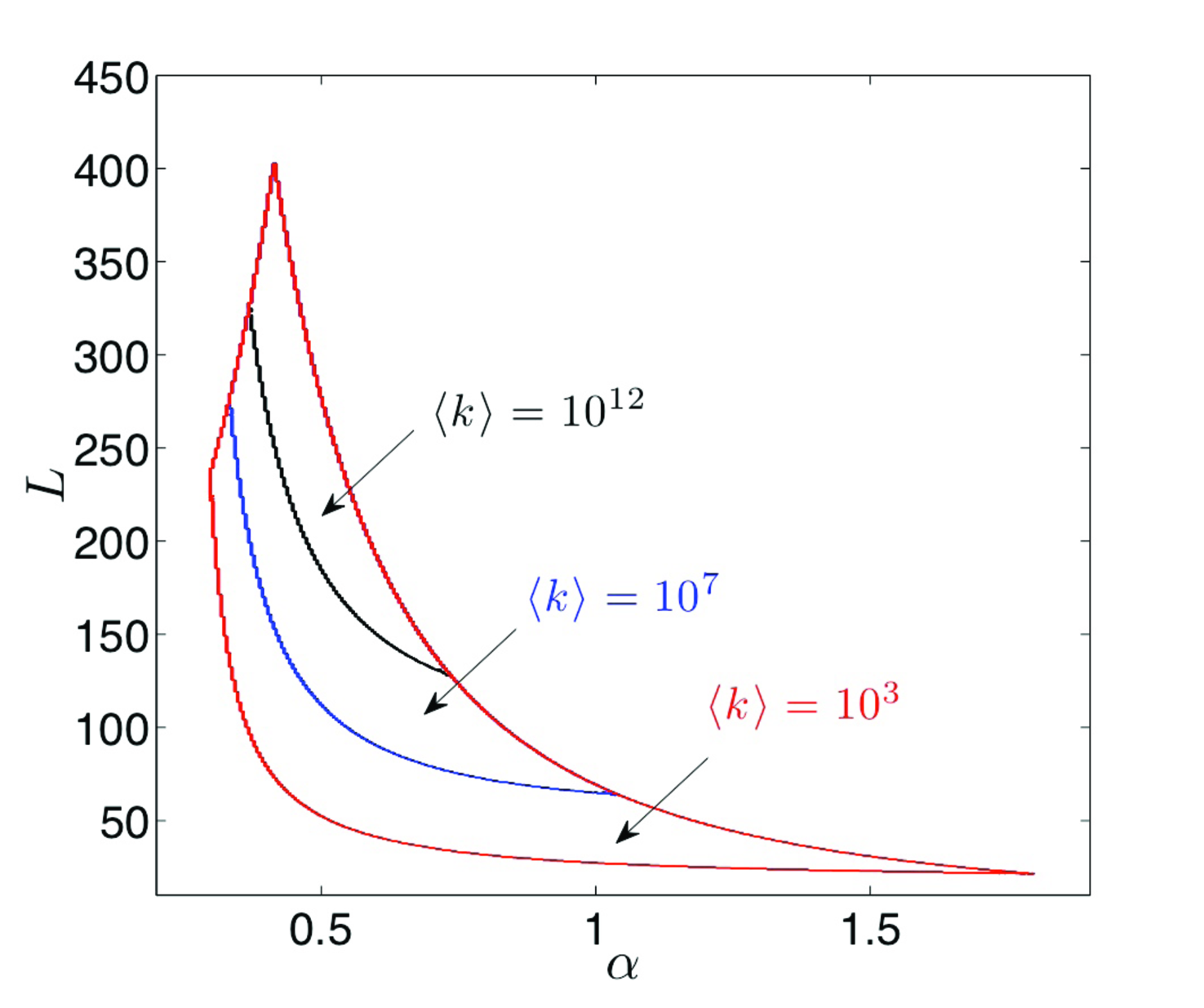
A better insight in the previous expression can be achieved from Fig. 4.4 which shows its numerical solution for different values of $\langle k\rangle$ (each shown in a different color): for a given average degree $\langle k\rangle$, the region of the plan $(\alpha,L)$ contained within the pertaining satisfies Eq. (4.10). For instance, let us assume $\langle k\rangle=10^{12}$ and $L=140$, then $\alpha$ must be not larger than approximately $0.75$ if we want that a response from the anti-anti-Ig follows the reaction of a specific Ig. By analyzing Fig. 4.4, wenotice that the less diluted the network the smaller the region of “retrieval”; Indeed, if we fix a given point on the $(\alpha,L)$, increasing $\langle k\rangle$ implies a larger $N$ and this contrasts with the satisfability of Eq. (4.10), on the other hand this result is rather intuitive as, when the coordination is large, the anti-antibody is less reactive with respect to the stimulus provided that the related antibody. As for the region corresponding to large $L$ and relative large $\alpha$, this never overlaps with the retrieval region, in fact for those values $\sigma_{\alpha,L}^{J}$ is relatively small.

Finally, we stress that when $\langle k\rangle$ is close to real values, i.e. $\mathcal{O}(10^{12})$ the retrieval region is centered on $L\sim 10^{2}$ and $\alpha$ between $0.5$ and $1$, this is consistent with the conclusions drawn from the analysis of the network dilution (Sec. 3.2) and from the analysis of sel/non-self recognition (Sec. 4.1).

4.5 Generation of memory cells

Figure 4.4: Numerical solution of Eq. (4.10): different values of $\langle k\rangle$ correspond to different closed curves, whose internal region provides the values of $\alpha$ and $L$ which satisfy the inequality of Eq. (4.10), namely the region of retrieval.

The last step we perform is to zoom inside the immune system and consider the behavior of single clones when stimulated with fields so to secrete immunoglobulins in high concentration; to this task, as the antigen concentration varies during the infection (at first increasing than -hopefully- decreasing) we have to deal with time dependent fields pushing the system away from the equilibrium. However for the sake of clearness at first we work out the equilibrium behavior of only two clones in interaction with each other and with their corresponding fields, so to have equilibrium even at this zoomed level, then, in the other sections, we will study their dynamical features.

Another interesting property of the immune system is the long-term memory of the past infections: When an antigen has been successfully rejected, part of the stimulated lymphocytes (corresponding to clones which have undergone expansion) do not recover the rest but they become "memory-cells", namely they remain activated, such that if the same antigen is re-introduced in the body an immediate, and highly specific response, usually improved with respect to the first time, can raise immediately.

The amount of memory cells achieved after an infection is not a constant and it is known to depend on the time of the infection and on the kind of the infection [9, 61].

We want to show that our model exhibits a phenomenon called "hysteresis" [42, 43] and this may account for the generation of the memory cells, furthermore it can model naturally both the improvement of the quality of the antibody production in the second response and the time-dependence in the ratio of the obtained memory-cells.

The hysteresis is a dynamical feature (disappearing in the quasi-static limit [41]) which essentially arises due to conflicting timescales inter-playing.

In ferromagnetic materials hysteresis is a well known phenomenon, both theoretically and experimentally: When an oscillating magnetic field is applied to a ferromagnet, the thermodynamic response of the system, namely its magnetization, will also oscillate and will lag behind the applied field due to the relaxational delay. Therefore, the two time-scales inter-playing are given by the frequency of the external field $\omega$ and by the thermalization of the system itself. When relaxation is slower than field oscillations we have a delay in the dynamic response of the system which gives rise to a non-vanishing area of the magnetization-field loop; this phenomenon is called dynamic hysteresis.

In an immune system the two dynamical phenomena and related time-scales involved are: the raise of the immune response (which may depend by the particular clone interested) and the antigenic growth (which strongly depends by the given antigen). When the two subjects are made interacting delays in the dynamic response gives rise to several interesting phenomena: at first when the concentration of the antigen is bring back to zero at the end of the fight, there can be not zero -remanent- magnetization (lacking of the in-phase behavior appears), further, if we deal with periodic perturbation, when the time period of such antigenic oscillations becomes much less than the typical relaxation time of the clone, a dynamical phase transition toward a chronic response may appear. Ultimately this approach may bridge the Barkhausen effect [41] to the "Jerne avalanches" of antibody and anti-antibody, whose distribution and sizes are interesting information.

Before results are outlined, we stress that we applied sinusoidal fields of the form $h(t)=h_{0}\sin(\omega t)$, where $h_{0}$ takes into account the interaction thought the lymphocyte network, while $\omega$ rules the timescale of the antigen.

4.6 Two clones dynamics and maturation of secondary response

Figure 4.5: Examples of hysteresis cycles for a two-body system: on the $y$-axis we show the concetration of firing lymphocytes and on the $x$-axis the amplitude of the external field. Two different frequences are considered: $\omega=0.1$ (left panel) and $\omega=0.01$ (right panel). The level of noise is below the critical value.

Figure 4.6: Hysteresis displayed by the stimulated best matching clone Ab1, a spurious clone Ab2 and the Jerne counterpart of Ab1, namely AAb1. From the picture the maturation of best performing response can be understood as follows: at the first infection with the antigen both the best matching clone (Ab1) and a spurious state (AAb1) are elicited. However Ab1 experiences an higher field such that its saturation in the hysteresis curve is greater with respect to Ab2 and so is its remanent magnetization. At the second infection of the same antigen the quiescent state is no longer the old one as now different concentrations of the two clones are stored and in particular Ab1 shows higher values than AAb1 so its response starts immediately higher and overall the immune response is stronger, due to both the remanent magnetization, and sharper, due to the mismatch among their relative concentrations.

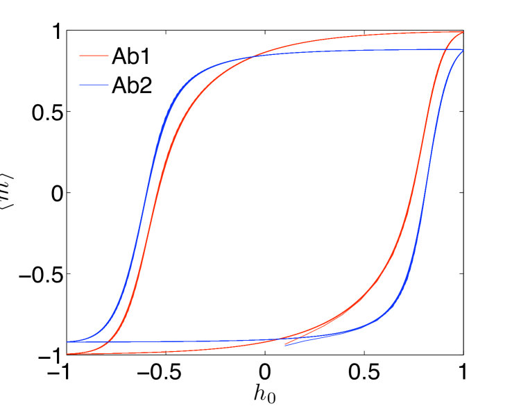
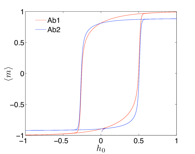
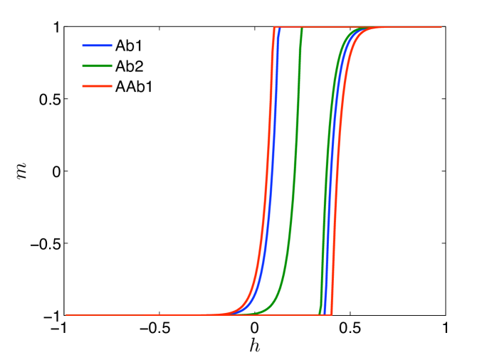
For simplicity, let us start considering only two clones ($N=2$) in interaction, as the generalization to slightly more involved situations (i.e. four clones) is straightforward. The macroscopic states of the two clones are $m_{1}=M^{-1}\sum_{\alpha=1}^{M}\sigma_{1}^{\alpha}$ and $m_{2}=M^{-1}\sum_{\alpha=1}^{M}\sigma_{2}^{\alpha}$.
Given these two clones, $i$ and $j$, their mutual interaction parameter $J_{ij}$ depends on the subset they belong to, as specified by the symmetric matrix

$$\begin{array}[]{ll}\\ P\left\{\begin{array}[]{ll}\\ \\ \end{array}\right.\\ P\left\{\begin{array}[]{ll}\\ \\ \end{array}\right.\end{array}\!\!\!\!\!\!\!\!\begin{array}[]{ll}\quad\overbrace{\qquad\qquad}^{\textrm{$P$}}\ \ \ \overbrace{\qquad\qquad}^{\textrm{$P$}}\\ \left(\begin{array}[]{cc|cc}\mathbf{J_{11}=0}&&\mathbf{J_{12}=J}\\ \\ \\ \mathbf{J_{12}=J}&&\mathbf{J_{22}=0}\\ \end{array}\right)\end{array}$$

where each matrix block has constant elements: $J_{11}=J_{22}=0$, as lymphocytes carrying the same idiotype do not interact, while $J_{12}=J_{21}>0$ controls the interaction between lymphocytes of different clones.

Analogously, the field $h_{i}$ takes two values $h_{1}$ and $h_{2}$, depending on the type of $i$, as described by the following vector:

$$\begin{array}[]{ll}M\left\{\begin{array}[]{ll}\\ \\ \end{array}\right.\\ M\left\{\begin{array}[]{ll}\\ \\ \end{array}\right.\!\!\!\!\!\!\end{array}\!\!\!\!\!\!\left(\begin{array}[]{cc|cc}\mathbf{h_{1}}\\ \\ \mathbf{h_{2}}\\ \\ \end{array}\right).$$

This model, two paramagnets ferromagnetically interacting, has two coupled self-consistence relations [31, 60] which solves the $t\to\infty$ limit of the stochastic dynamics, worked out as

$$\frac{dm_{1}(t)}{dt}=-m_{1}(t)+\tanh\Big{(}\beta(J_{12}m_{2}(t)+h_{1}(t))\Big{)},$$ (4.11)

$$\frac{dm_{2}(t)}{dt}=-m_{2}(t)+\tanh\Big{(}\beta(J_{12}m_{1}(t)+h_{2}(t))\Big{)}.$$ (4.12)

Despite its simplicity the phase diagram of these two interacting clones is already rich of both continuous and discontinuous transitions [31, 60] and is found to have not trivial stable concentrations of the clones accounting for the optimality of the free energy density.

Figure 4.7: Examples of bell-shaped response for a $2$-clones system

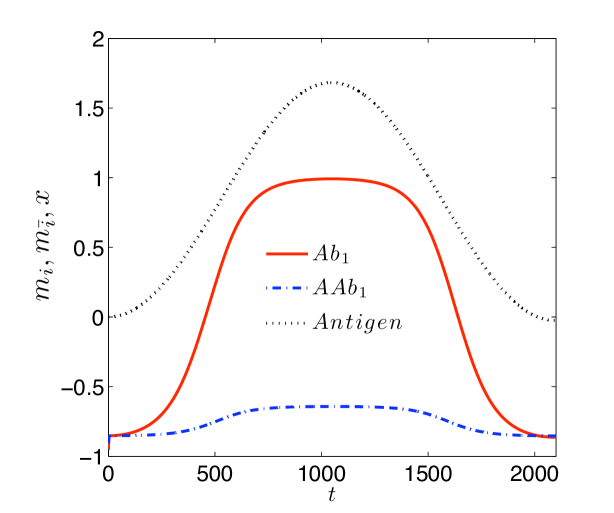
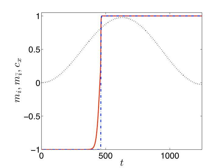
To accomplish our task we start applying a field $h$ to the immune system at rest and collect the responding clones.

For these clones we generalize the Langevin equation of the two-body model (eq.s 4.11,4.12) so to obtain a system of coupled stochastic equations (one for each order parameter of a stimulated clone) that we integrate via the step adaptive Runge-Kutta algorithm [69].
Roughly speaking, if we define -as a measure of the out-of-phase response- the area of the hysteresis loop in the $h_{i},m_{i}$ plane as

$$A(\beta,h_{0},\omega)=\oint mdh$$

we found that this area is increasing with $\omega$ at low frequencies (because increasing the frequency increases the delay), then reaches a maximum and than start decreasing (due to the $2\pi/\omega$ periodicity); when looking at this area versus the noise level it is seen to increase when $\beta$ increases (that means that the affinity matrix can be more felt by the system and consequently its delay increases because of the storing of information inside the relative coupling concentrations). In figure (4.6) we show a typical behavior (for $\beta<\beta_{c}$) of the first two best fitting clones elicited by an external antigen: A proposal for the understanding of the improvement of both the quantity and the quality of the secondary response can be obtained from the picture.

The secondary immune response is stronger because the best fitting lymphocyte (Ab1) at the second infection do not start off from the minimal allowed value (as the first time) but from the value of concentration related to the remanent magnetization. It is also more specific than the first response. This can be understood by the following argument: At the beginning all the clones start off from the quiescent values. However, the lymphocyte with the best fitting antibody experiences an eliciting field stronger than the others (in particular than AAb1) and so it reaches saturation in the hysteresis for a longer time. This allows a greater remanent magnetization with respect to the spurious state which expanded as well. As a consequence, if the stimulus is presented once again, the immune system is not simply translated from quiescence level of concentrations to remanent magnetization levels, but different values of the latter, among Ab1 and AAb1, account for an improved response.

4.7 Bell shaped response

In this section we want to show that, within our model, the so called "bell-shaped response" [9] is recovered as the typical immune response.

As we are interested in basic features of the immune system, we look at the two most common responses to only the positive half of a sinusoidal stimulus: the two-clone circuit and the four-clone circuit, which naturally extend the Eqs. (4.11, 4.12), the only difference being the coupling field which by now acts only on $m_{1}$ (whose concentration we want to measure).

Figure 4.8: Examples of bell-shaped response for a $4$-clones system

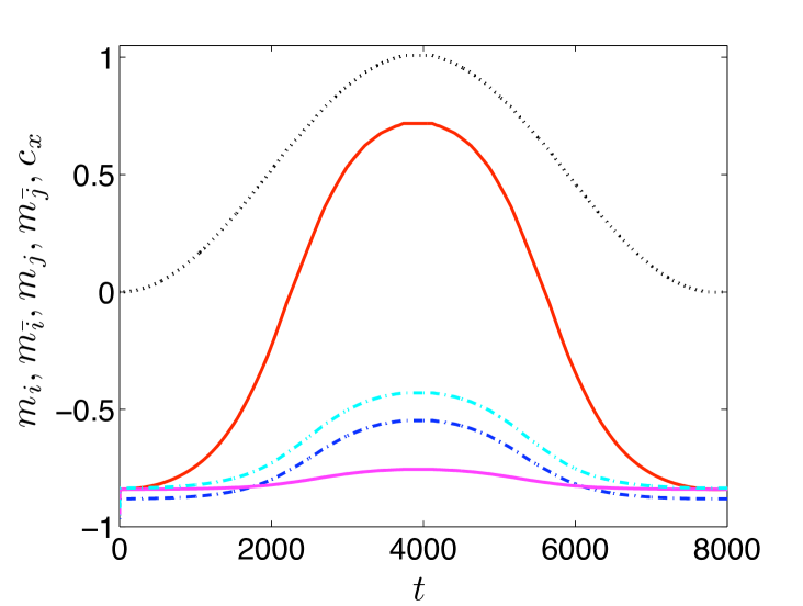
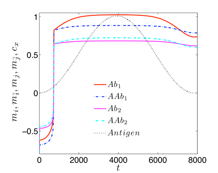
Before presenting our results it is worth spending few lines to introduce more clearly our approach: usually when dealing with these dynamical features of the immune system, the most intuitive way is to work out time-differential equations for the evolution of the antigenic and antibody concentrations (which is indeed what is almost always done [49, 70, 71]. This account for $m(t)$ and $h(t)$, then one, carefully looking at the monotonic regions of the two behaviors, can parameterize and get $m(h)$. Within our approach we do not solve this kind of problem, instead we directly give an expression for the antigenic load and then we obtain $m(h)$ as a result. This has two advantages: this allows to deal with Fourier analysis, furthermore this skips all the troubles about the details of the interactions which may strongly depend on the particular antigen [9]. Of course we pay the price of testing these responses with ideal mono-frequency viruses which are surely an oversimplification: however a more complex behavior can be obtained considering the antigen as a sum of several perturbing harmonics, which is allowed due to the linearity of the Hamiltonian $H_{1}$ with respect to the fields.

Typical results of bell-shaped found at different field frequency and magnitude are presented in the panels of Fig. 4.7 and of Fig. 4.8 .

Chapter 5 Conclusions and Perspectives

5.1 Summary

In this paper we pioneered an alternative way to theoretical immunology by plugging it into a concrete disordered statistical mechanics framework: our work is not meant as an exhaustive picture of the (adaptive response of the) immune system, but rather as a starting point in modeling its universal features by means of this technique.

We stress that, in our model, once the amount of available epitopes and their distributions is given (namely the amount of $\xi$’s together with their distribution), everything can be worked out. This way, we recover, qualitatively and partially quantitatively, all the basic known features of the immune system and we obtain a good agreement with experimental data, starting with a reasonable amount of working lymphocytes and antibody concentrations.

In particular, in the complex system framework we developed, the immune network naturally and autonomously achieves/recovers the following properties:

• the Burnet clonal expansion theory [4][33] appears as the standard one-body response of the system described by the Hamiltonian $(2.5)$ (remembering the bridge among magnetization and concentration encoded into eq. $(2.4)$).

• the multi-attachment among antibodies is a natural property of the system and gives raise to the Jerne network (cfr. eq.(3.3))

• the Jerne antibody network, which is obtained as a random graph, encodes dynamically the memory of the encountered antigens (see fig.$(3.4)$ and fig. $(4.4)$).

• the Varela-Counthino self/non-self distinction appears as an emerging property of such a network (see fig. $(3.6)$ and fig. $(4.1)$).

• the Low Dose Tolerance is the inertia of the network when subjected to respond to external fields (see fig. $(4.2)$).

• the existence of several antibodies acting against a given antigen, play the role of the dynamical spurious states of the neural network static counterpart (see fig. $(4.3)$).

• the High Dose Tolerance appears as a mechanism avoiding the breaking of self-recognition (see sec. $(4.2)$).

• the genesis of memory cells (accounting for the transition IgG -> IgM in antibody secretion) is played by the hysteresis in the network (see fig. $(4.5)$).

• the bell-shaped function as immune response is an emergent behavior and not a postulate (see fig. $(4.7)$ and fig. $(4.8)$).

• the secondary response is stronger and better than the first (see fig. $(4.6)$).

• increasing the noise, both the the quality and the quantity of the available retrievals decrease.

All these different aspects of the immune system appear as features of a whole unified quantitative and very simple theory. Furthermore, over these agreements, matching with the experimental data is available: namely the average connectivity of the network is in agreement with the experiments as well as the reciprocal affinities of the cascade of complementary antibodies.

With purely physical eyes our model describes the equilibrium of the immune system as a (thermodynamically [34]) symmetry broken random bond diluted ferromagnet. However, its non equilibrium states map the latter into a random field random bond diluted model, conferring to the system a glassy flavor.

5.2 Outlooks

Among the several outlooks surely the out of equilibrium thermodynamics is to be obtained as the model is shown to display a very rich ensemble of timescales and aging is expected. Another important point is its learning, that so far is left uninvestigated, which merges the approach of neural networks [19] and the dynamical graph theory with information theory. The extension of the concept of Hopfield statical memories into a dynamical counterpart should be deepened as well as the Gardner saturation bound [11], which may play a key role in the breaking of defense in the body. The transition from a "simple" system to a "spin glass" due to the increase of pasted random fields also needs a deep analysis as it is concerned with the genesis of autoimmune responses. The interplay among B cells and T helper cells should also be taken into account as T helper play the role of a spin glass self-regulation adding a considerable amount of complex self-regulations. At the end, as our results are qualitatively quite robust and the framework very stable under the change in the epitope distributions, other, mathematically challenging (i.e. due to correlations), choices for these distributions are surely biological plausible and should be investigated. We plan to report soon on several of the outlines directions of research.

Acknowledgment

The author are grateful to O. Barra, R. Burioni, M. Casartelli, P. Contucci, A.C.C. Coolen, S. Franz, F. Guerra, G. Ruocco and N. Shayeghi for useful discussions.

References

- [1] F. Celada, Search of T-cell help for the internal image of the antigen, Theor. Imm. 2, A.S. Perelson Ed. Addison-Wiley Pubbl. (1988).
- [2] V.G. Nesterenko, Symmetry and asimmetry in the immune network, Theor. Imm. 2, A.S. Perelson Ed. Addison-Wiley Pubbl. (1988).
- [3] L.A. Segel, A.S. Perelson, Computations in shape space: A new approach to immune network theory, Theor. Imm. 2, A.S. Perelson Ed. Addison-Wiley Pubbl. (1988).
- [4] F.M. Burnet, The clonal selection theory of acquired immunity, Vanderbilt Univ. Press. Nashville, (1959).
- [5] F.M. Burnet, F. Fenner, The production of antibodies, MacMillan Ed.s, Melbourne (1949).
- [6] P. Elrich, Studies in Immunity, Wiley, New York, (1910).
- [7] W.J. Dreyer, J.C. Bennett, Molecular bases of antibody formation: a paradox, Nobel Prize Lecture, (1965).
- [8] G.W. Hoffmann, A theory of regulation and Self-NonSelf discrimination in an immune network, Eur. J. of Imm. 5, 638-643, (1975).
- [9] A. K. Abbas, A. H. Lichtman, J. S. Pober, Cellular and molecular immunology, Elsevier Ed.s, (2007).
- [10] E. Agliari, A. Barra, F. Camboni, Criticality in diluted ferromagnets, J. Stat. Mech., (2008).
- [11] D.J. Amit, Modeling brain function: The world of attractor neural network Cambridge Univerisity Press, (1992)
- [12] D.J. Amit, H. Gutfreund, H. Sompolinsky, Storing infinite numbers of patterns in a spin glass model of neural networks, Phys. Rev. Lett. 55, (1985).
- [13] R. Albert, A. L. Barabasi Statistical mechanics of complex networks, Reviews of Modern Physics 74, 47-97 (2002).
- [14] A. Barra, The mean field Ising model trhought interpolating techniques, J. Stat. Phys. 132, (2008).
- [15] A. Barra, Irreducible free energy expansion and overlap locking in mean field spin glasses, J. Stat. Phys. 123, (2006).
- [16] A. Barra, F. Guerra, About the ergodicity in Hopfield analogical neural network, J. Math. Phys. 50, (2008).
- [17] A. Barra, F. Camboni, P. Contucci, Structural stability of dilution in mean field models, J. Stat. Mech., P03028, (2009).
- [18] A. Barra, G. Genovese, An analytical approach to mean field systems defined on lattice, J. Math. Phys. 51, (2009).
- [19] A.C.C. Coolen, R. Kuehn, P. Sollich, Theory of Neural Information Processing Systems, Oxford Univ. Press, (2005).
- [20] H. Jacobs, L. Bross, Towards an understanding of somatic hypermutation, Current Opinion in Immunology 13, 208-218, (2001).
- [21] U. Storb, The molecular basis of somatic hypermutation of immunoglobulin genes, Curr. Op. in Imm. 8, 206-214, (1996).
- [22] I. Lundkvist, A. Coutinho, F. Varela, D. Holmberg, Evidence for a functional idiotypic network among natural antibodies in normal mice, P.N.A.S. 86, , (1989).
- [23] M. Mézard, G. Parisi and M. A. Virasoro, Spin glass theory and beyond, World Scientific, Singapore (1987).
- [24] J.M. Seigneurin, B. Guilbert, M.J. Bourgeat, S. Avrameas, Polyspecific natural antibodies and autoantibodies secreted by human lymphocytes immortalized with Epstein-Barr virus , Blood, 71, 3, 581-585, (1988).
- [25] G. Parisi, A simple model for the immune network, P.N.A.S. 87, .
- [26] P. Pereira, L. Forni, E.L. Larsson, M. Cooper, C. Heusser, A. Coutinho, Autonomous activation of B and T cells in antigen free mice, Eur. Journ. Immun., 16, (1986).
- [27] J. Stewart, F. J. Varela, A. Coutinho, The relationship between connectivity and tolerance as revealed by computer simulation of the immune network: some lessons for an understanding of autoimmunity, J. of Autoimmunity, 2, (1989).
- [28] F.J. Varela, A. Countinho, Second generation immune networks, Imm. Today 12, 5, 159, (1991).
- [29] Edelman, G.M., The problem of molecular recognition by a selective system, In Ayala/Dobzhansky, Studies in the Philosophy of Biology, , (1974).
- [30] Ledemberg, Genes and antibodies, Nobel Prize Lecture.
- [31] I. Gallo, P. Contucci Bipartite mean field spin systems. Existence and solution , Math. Phys. E. J. 14, (2008).
- [32] N.K. Jerne, Toward a network theory of the immune response, Ann. Imm. 125, C, (1974).
- [33] F.M. Burnet, A modification of Jerne’s theory of antibody production using the concept of clonal selection, Australian J. Science 20,, 67, (1957).
- [34] A. Cooper-Willis, G.H. Hoffmann. Symmetry of effector function in the immune system network, Mol. Imm. 20, 865, (1983).
- [35] H. C. Tuckwell, Introduction to theoretical neurobiology, Cambridge St. Math. Bio., Cambridge Press, (1988).
- [36] L. DeSanctis, F. Guerra, The dilute ferromagnet: high temperature and zero temperature, J. Stat. Phys. 132, (2008).
- [37] J.P.L. Hatchett, I. Pérez Castillo, A.C.C. Coolen, N.S. Skantzos, Dynamical replica analysis of disordered Ising spin systems on finitely connected random graphs, Phys. Rev. Lett. 95, 117204, (2005).
- [38] H. Lemke, H. Lange,Generalization of single immunological experiences by idiotypically mediated clonal connections, Adv. Immunol. 80, 3078-3082, (1980).
- [39] M. Molloy and B. Reed, A critical point for random graphs with a given degree sequence, Random Structures and Algorithms 6, 161-180, (1995).
- [40] A. Nachmias and Y. Peres, Component sizes of the random graph outside the scaling window, Alea 3, 133-142, (2007).
- [41] B.K. Chakrabarti, M. Acharyya, Dynamic transitions and hysteresis, Rev. Mod. Phys. 71, 3, (1999).
- [42] K.F. Ludvig, B. Park, Kinetics of true-field Ising models and the Langevin equation: A comparison, Phys. Rev. B, 46, 9, (1992).
- [43] J.O. Sethna, K. Dahmen, S. Kartha, J.A. Krumhansl, B.W. Roberts, J.D. Shore, Hysteresis and hierarchies: Dhyamics of disorder-driven first-order phase transformations, Phys. Rev. Lett. 70, 21, (1993).
- [44] L.A. Segel, A.S. Perelson, Shape space: an approach to the evaluation of cross-reactivity effects, stability and controllability in the immune system, Imm. Lett. 22, 91-100, (1989).
- [45] J. Chun, Selected comparison of immune and nervous system development, Adv. Imm. 77, (2001).
- [46] P.M. Colman, Structure of antibody-antigen complexes: implication for immune recognition, Adv. Imm. 43, (1988).
- [47] P.A. Cazenave, Idiotypic-anti-idiotypic regulation of antibody synthesis in rabbits, P.N.A.S. 74, vol 11, 5122-5125, (1977).
- [48] W.E. Paul, C. Bona, Regulatory idiotopes and immune networks: a hypothesis, Imm. Today 3, 9, (1982).
- [49] R.J. De Boer, Symmetric idiotypic networks: connectance and switching, stability and suppression, Theor. Immun. Vol., Studies in the sciences of complexity, Add.-Wiley Publ. (1988).
- [50] E. Agliari, A. Barra, F. Camboni, Criticality in diluted ferromagnets, J. Stat. Mech. P1003 (2008).
- [51] R.S. Ellis, Large deviations and statistical mechanics, Springer, New York (1985).
- [52] F. Guerra, F. L. Toninelli, The high temperature region of the Viana-Bray diluted spin glass model, J. Stat. Phys. 115, (2004).
- [53] M.Mezard, G.Parisi, R. Zecchina, Analytic and Algorithmic Solution of Random Satisfiability Problems, Science 297, 812 (2002).
- [54] M. Newman, D. Watts, A.-L. Barabasi The Structure and Dynamics of Networks, Princeton University Press, (2006).
- [55] A.C.C. Coolen, The Mathematical Theory of Minority Games - Statistical Mechanics of Interacting Agents, Oxford University Press, (2005).
- [56] Durlauf, S. N.: 1999, How can statistical mechanics contribute to social science?. Proceedings of the National Academy of Sciences of the U.S.A. 96, 10582-10584, (1999).
- [57] Mc Fadden, D. (2001), Economic Choices, The American Economic Review, 91: 351-378, (2001)
- [58] M. Mézard, G. Parisi and M. A. Virasoro, Spin glass theory and beyond, World Scientific, Singapore (1987).
- [59] G. Semerjian, M. Weigt Approximation schemes for the dynamics of diluted spin models: the Ising ferromagnet on a Bethe lattice J. Phys. A 37, (2004).
- [60] A. Barra, G. Genovese, A certain class of Curie-Weiss models, Math. Phys. El. J. (2010).
- [61] P. Delves, S. Martin, D Burton, I Roitt, Roitt’s Essential Immunology, Wiley Ed.r, (2006).
- [62] P. Sollich, Soft glassy rheology, Phys. Rev. E
- [63] N.R. Rose, I.R. Mackay, The autoimmune diseases, Elsevier Press, (2006).
- [64] F. Mandl, G. Shaw, Quantum field theory, Wiley Ed.r, (1984).
- [65] J. Monod, Chance and Necessity, A. Knopf Ed.r, New York, (1971).
- [66] R. J. Bagley, J.D. Farmer, N.H. Packard, A.S. Perelson, I.M. Stadnyk, Modeling adaptive biological systems, Biosystems. 23, 113-138, (1989).
- [67] J. D. Farmer, A. Lapedes, N.H. Packard, B. Wendross, Evolution, Games and Learning, eds. North-Holland, (1987).
- [68] S.C. Bagley, H. White, B.A. Golomb, Logistic regression in the medical literature, J. Clin. Epidem. 54, 10, (2001).
- [69] D. Frenkel, B. Smith, Understanding molecular simulation, Elsevier Press, (2002).
- [70] R.J. Be Boer, I.G. Kewrekidis, A.S. Perelson em Immune network behavior. From stationary to limit cycle oscillations, Bull. Math. Biol, 55, 745-780 (1993).
- [71] G,W, Hoffmann, T.A. Kion, R.B. Forsyth, K.G. Soga,A. Cooper-Willis, The -dimensional network, Theor. Imm. 2, A.S. Perelson Ed.r, Addison-Wiley Pubbli., (1988).
- [72] D.Holmberg, G. Wennerström, L. Andrade and A. Coutinho The high idiotypic connectivity of ‘natural’ newborn antibodies is not found in adult mitogen-reactive B cell repertoires, Eur. J. Immunol. 16, 82-87 (1986).
- [73] V. Detours, B. Sulzer and A. Perelson, Size and Connectivity of the Idiotypic Network Are Independent of the Discreteness of the Affinity Distribution, J. Theor. Biol. 183, 409-416, (1996).