Wormholes or Gravastars?

Abstract

The one loop effective action in a Schwarzschild background is here used to compute the Zero Point Energy (ZPE) which is compared to the same one generated by a gravastar. We find that only when we set up a difference between ZPE in these different background we can have an indication on which configuration is favored. Such a ZPE difference represents the Casimir energy. It is shown that the expression of the ZPE is equivalent to the one computed by means of a variational approach. To handle with ZPE divergences, we use the zeta function regularization. A renormalization procedure to remove the infinities together with a renormalization group equation is introduced. We find that the final configuration is dependent on the ratio between the radius of the wormhole augmented by the ”brick wall” and the radius of the gravastar.

I Introduction

Black holes are well accepted astrophysical objects by scientific community. The simplest example of a black hole is the spherically symmetric vacuum solution of the Einstein field equations,

$$ds^{2}=-\left(1-\frac{2MG}{r}\right)dt^{2}+\frac{dr^{2}}{1-\frac{2MG}{r}}+r^{2}\left(d\theta^{2}+\sin^{2}\theta d\phi^{2}\right),$$ (1)

known as the Schwarzschild solution. Despite of many theoretical and observational successes, a number of paradoxical problems connected to black holes also existWald , which frequently motivate authors to look for other alternatives, in which the endpoints of gravitational collapse are massive stars without horizons. In 2001, Mazur and MottolaMM proposed an alternative model to black hole as a different final state of a gravitational collapse. In this model, the strong gravitational forces induce a vacuum rearrangement in such a way to avoid a classical event horizon. A phase transition is associated to the quantum gravitational vacuum together with a topology change. Such a model has been termed gravastar (gravitational vacuum star) and it consists of three different regions with three different Eqs. of state

$$\begin{array}[c]{rrr}I.\qquad\mathrm{Interior:}&0\leq r<r_{1}&\rho=-p,\\ II.\qquad\mathrm{Thin}\text{ }\mathrm{Shell:}&r_{1}<r<r_{2}&\rho=+p,\\ III.\qquad\mathrm{Exterior:}&r_{2}<r&\rho=p=0.\end{array}$$ (2)

At the interfaces $r=r_{1}$ and $r=r_{2}$, we require the metric coefficients to be continuous, although the associated first derivatives must be discontinuous. Globally the metric can be cast into a form very close to the Schwarzschild line element $\left(\ref{Schw}\right)$

$$ds^{2}=-N^{2}\left(r\right)dt^{2}+\frac{dr^{2}}{1-\frac{b\left(r\right)}{r}}+r^{2}\left(d\theta^{2}+\sin^{2}\theta d\phi^{2}\right),$$ (3)

where

$$N^{2}\left(r\right)=1-\frac{\Lambda_{dS}}{3}r^{2}\qquad\mathrm{and\qquad}b\left(r\right)=\frac{\Lambda_{dS}}{3}r^{3}$$ (4)

for the interior region of a static de Sitter metric, while

$$N^{2}\left(r\right)=1-\frac{2MG}{r}\qquad\mathrm{and\qquad}b\left(r\right)=2MG$$ (5)

for the exterior region described by a Schwarzschild spacetime. The intermediate region is represented by a thin shell endowed with a Minkowski metric. However, the thin shell is by no means necessary to obtain a gravastar. Indeed, DeBenedictis et al. DBHIKV proved that the shell region can be eliminated and the de Sitter spacetime can be directly joined to the Schwarzschild metric. This picture was also considered by DymnikovaDymnikova without invoking the term “gravastar”. From the asymptotic point of view, a gravastar and a black hole share the same Arnowitt-Deser-Misner ($\mathcal{ADM}$) massADM , therefore at very large distances they appear the same object to an observer. One may wonder how can we distinguish a black hole from a gravastar. Different proposal have been considered. Harko et al.HKL suggested to compare the thermodynamical and electromagnetic properties of the accretion disk around slowly rotating black holes and gravastars. Another proposal comes from Chirenti and RezzollaCR , where the use of axial perturbations and the analysis of Quasi Normal Modes seems to show how to distinguish a black hole from a gravastar. Cardoso et al.CPCC discussed the ergoregion instability produced by rapidly spinning compact objects such as gravastars and boson stars with the results that ultra-compact objects with large rotation are black holes. On the other side, Chirenti and RezzollaCR1 found that stable models can be constructed also with $J/M^{2}\sim 1$, where $J$ and $M$ are the angular momentum and mass of the gravastar, respectively. Note that the comparison between a gravastar and a black hole is at the classical level, without any quantum contribution which should also be the source of the desired phase transition to make a gravastar. Note also that, in principle there exists another source of ambiguity: indeed besides a gravastar and a black hole, the exterior metric can be associated to a wormhole. In this paper, we would like to compare a gravastar to a wormhole. From the asymptotic point of view even the wormhole shares the same $\mathcal{ADM}$ mass. Hence, it should be very important the comparison of such objects invoking the Zero Point Energy (ZPE) contribution. However, it is well known that every form of ZPE also contributes to an induced cosmological constant. If we indicate with $E_{0}^{GS}$ the gravastar ZPE and with $E_{0}^{W}$, the wormhole ZPE, in principle one can discuss the following inequalities

$$\left(E_{0}^{W}-E_{0}^{GS}\right)\gtreqless 0$$ (6)

establishing which geometry is energetically favored compared to the other one. Essentially, this is a Casimir-like calculation and lower the ZPE, the more stable is the final configuration. This inequality is also related to the decay probability per unit volume and time $\Gamma$, which is defined as

$$\Gamma=A\exp\left(-I_{cl}\right)=\exp\left(-I_{g}\left[\bar{g}_{\mu\nu}\right]\right)\int\mathcal{D}h_{\mu\nu}\exp\left(-I_{g}^{\left(2\right)}\left[h_{\mu\nu}\right]\right),$$ (7)

for an Euclidean time. Indeed, at least a tree level, we find that

$$\Gamma\simeq\exp\left(-I_{cl}\right)=\exp\left(-\left(E_{0}^{GS}-E_{0}^{W}\right)\Delta\tau\right),$$ (8)

where $\Delta\tau$ is the Euclidean time interval. Basically, the first step is the evaluation of the following expectation value

$$\left\langle T_{\mu\nu}\right\rangle=\frac{2}{\sqrt{-g}}\frac{\delta\Gamma_{g}}{\delta g^{\mu\nu}},$$ (9)

provided one can compute the effective action related to $S_{g}$. To do calculations in practice, we fix our attention to the standard Einstein action without matter fields and with a cosmological term

$$S=S_{g}+S_{C.C.}$$ (10)

where

$$S_{g}=\frac{1}{16\pi G}\int d^{4}x\sqrt{-g}R,\qquad S_{C.C.}=-\frac{\Lambda}{8\pi G}\int d^{4}x\sqrt{-g}.$$ (11)

The least action principle leads to the Einstein’s fields equations with a cosmological term. Nevertheless, never forbids to consider the cosmological term as the desired induced quantity by ZPE. Therefore, Eq.$\left(\ref{eff}\right)$ must be modified into

$$\left\langle T_{\mu\nu}^{C.C.}\right\rangle=-\frac{2}{\sqrt{-g}}\frac{\delta\Gamma_{g}}{\delta g^{\mu\nu}}.$$ (12)

If we define the path integral

$$Z=\int\mathcal{D}\left[g_{\mu\nu}\right]\exp iS_{g}\left[g_{\mu\nu}\right]$$ (13)

and we consider a gravitational field of the form

$$g_{\mu\nu}=\bar{g}_{\mu\nu}+h_{\mu\nu},$$ (14)

then Eq.$\left(\ref{p01}\right)$ becomes

$$\int\mathcal{D}g_{\mu\nu}\exp iS_{g}\left[g_{\mu\nu}\right]=\exp iS_{g}\left[\bar{g}_{\mu\nu}\right]Z_{2}=\exp iS_{g}\left[\bar{g}_{\mu\nu}\right]\int\mathcal{D}h_{\mu\nu}\exp iS_{g}^{\left(2\right)}\left[h_{\mu\nu}\right],$$ (15)

where we have assumed that the background $\bar{g}_{\mu\nu}$ is a solution of the Einstein field equations and

$$S_{g}^{\left(2\right)}\left[h_{\mu\nu}\right]=\frac{1}{2\kappa}\int_{\mathcal{M}}d^{4}x\sqrt{-g}h_{\mu\rho}O^{\mu\rho\sigma\nu}\!{}h_{\sigma\nu}$$ (16)

with $\kappa=8\pi G$. $O^{\mu\rho\sigma\nu}$ is a symmetric tensor operator with

$$O^{\mu\rho\sigma\nu}=\frac{\delta^{2}S\left[\bar{g}_{\mu\nu}\right]}{\delta h^{\mu\rho}\delta h^{\sigma\nu}}$$ (17)

and $h_{\sigma\nu}$ is the quantum fluctuation with respect to the background $\bar{g}_{\sigma\nu}$. After some integration by parts, Eq.$\left(\ref{quadr}\right)$ becomes

$$S^{\left(2\right)}=\frac{1}{2\kappa}\int_{\mathcal{M}}d^{4}x\sqrt{-g}\left[-\frac{1}{4}h^{\mu\nu}\left(\bigtriangleup_{L\!}\!{}h\right)_{\mu\nu}+\frac{1}{4}h\bigtriangleup\!{}h+h^{\mu\rho}R_{\rho\nu}h_{\mu}^{\nu}-\frac{1}{2}h^{\mu\nu}\!{}h_{\mu;\alpha;\nu}^{\alpha}\right.$$

$$\left.-\frac{1}{2}hR_{\alpha\beta}h^{\alpha\beta}+\frac{1}{2}h\!{}h_{;\mu;\nu}^{\mu\nu}+R\left(-\frac{1}{4}h^{\mu\nu}h_{\mu\nu}+\frac{1}{8}h^{2}\right)\right].$$ (18)

$\bigtriangleup_{L}$stands for the Lichnerowicz operator defined by

$$\left(\bigtriangleup_{L}h\right)_{\mu\nu}=-\nabla^{a}\nabla_{a}h_{\mu\nu}-2R_{\mu\alpha\nu\beta}h^{\alpha\beta}+R_{\mu\alpha}h_{\nu}^{\alpha}+R_{\nu\alpha}h_{\mu}^{\alpha}=\bigtriangleup h_{\mu\nu}-2R_{\mu\alpha\nu\beta}h^{\alpha\beta}+R_{\mu\alpha}h_{\nu}^{\alpha}+R_{\nu\alpha}h_{\mu}^{\alpha},$$ (19)

where we have introduced the positive definite differential operator

$$\bigtriangleup=-\nabla^{a}\nabla_{a}.$$ (20)

$S^{\left(2\right)}$ simplifies considerably when we are on shell, namely $R_{\alpha\beta}=0$. Nevertheless, for future purposes, it is convenient keeping such terms in the expression of the Lichnerowicz operator and in Eq.$\left(\ref{S24d}\right)$. To extract physical informations from expression $\left(\ref{p02}\right)$, we need an orthogonal decomposition which is equivalent to the Faddeev-Popov procedure, at least to one loop. From Appendix A, we obtainGP ; CD

$$\Gamma_{1-loop}=\frac{i}{2}\left[Tr\ln\bigtriangleup_{L\!}^{\bot}\!-Tr\ln\triangle_{V^{\bot}}\right]=\frac{i}{2}\int_{\mathcal{M}}d^{4}x\sqrt{-g}\left[\int\frac{d^{4}k}{\left(2\pi\right)^{4}}\ln\lambda_{TT}^{2}-\int\frac{d^{4}k}{\left(2\pi\right)^{4}}\ln\lambda_{V^{\bot}}^{2}\right],$$ (21)

where $\lambda_{TT}^{2}$ and $\lambda_{V^{\bot}}^{2}$ are the eigenvalues of the Lichnerowicz operator for TT tensors and the transverse vector operator respectively. With the help of Eq.$\left(\ref{G1L}\right)$, Eq.$\left(\ref{effCC}\right)$ simply becomes

$$\left\langle T_{\mu\nu}^{C.C.}\right\rangle=-\frac{i}{2}g_{\mu\nu}\left[\int\frac{d^{4}k}{\left(2\pi\right)^{4}}\ln\lambda_{TT}^{2}-\int\frac{d^{4}k}{\left(2\pi\right)^{4}}\ln\lambda_{V^{\bot}}^{2}\right]$$ (22)

and if we identify

$$\frac{\Lambda}{8\pi G}=-\frac{i}{2}\left[\int\frac{d^{4}k}{\left(2\pi\right)^{4}}\ln\lambda_{TT}^{2}-\int\frac{d^{4}k}{\left(2\pi\right)^{4}}\ln\lambda_{V^{\bot}}^{2}\right],$$ (23)

we can interpret the cosmological constant as induced by quantum fluctuations of the gravitation field itself. Therefore, it is clear that inequality $\left(\ref{ineq}\right)$ can be directly measured by the induced cosmological quantity of Eq.$\left(\ref{LoverG}\right)$. Moreover this identification will be useful for the removal of divergences. A first observation about Eq.$\left(\ref{G1L}\right)$ is in order. Note that nothing has been said regarding the famous conformal factor problem. From this point of view, we adopt the approach of Mazur and MottolaMM1 in decomposing the gravitational perturbation. The super-metric free parameter “$C$” of Eq.$\left(\ref{superm}\right)$ leaves us the freedom to select the correct range in such a way the functional integration be convergent. Coming back to the Lichnerowicz operator $\left(\ref{dl4d}\right)$, one immediately recognize that finding the eigenvalues is not a trivial task in general. It is therefore necessary to adopt a convenient choice to manage Eq.$\left(\ref{Tmn}\right)$. In a previous work we approached the cosmological constant problem with the help of the Wheeler-DeWitt Equation cast in the form of a Sturm-Liouville problemRemo . Essentially the cosmological constant is reinterpreted as an eigenvalue, calculated in a Hamiltonian formalism breaking the covariance of space-time. In the next section, we adopt the same strategy provided one looks at the true degrees of freedom. The paper is organized as follows: in section II, we reduce the effective action by restricting the modes of the perturbation, in section III, we evaluate the functional determinants by means of a W.K.B. method, in section IV we compute the ZPE energy for the gravastar and the wormhole respectively and we compare them. Finally, in section V we conclude.

II Reducing the one loop effective action in 3+1 dimensions

How the Lichnerowicz operator decomposes in 3+1 dimensions it depends on the way one separates space from time. The $\mathcal{ADM}$ variables offer a valid example of such a decomposition. In terms of these variables, the metric background written in Eq.$\left(\ref{metric}\right)$ becomes

$$ds^{2}=-N^{2}dt^{2}+g_{ij}\left(N^{i}dt+dx^{i}\right)\left(N^{j}dt+dx^{j}\right).$$ (24)

We recognize that the lapse function $N$ is invariant and the shift function $N_{i}$ is absent. To have an effective reduction of the modes, we consider perturbations of the gravitational field on the hypersurface $\Sigma\subset\mathcal{M}$. This means that we are “freezing” the perturbation of the lapse and the shift functions respectively. In summary,

$$\left\{\begin{array}[c]{c}g_{ij}\longrightarrow\bar{g}_{ij}+h_{ij}\\ N\longrightarrow N\\ N_{i}\longrightarrow 0\end{array}\right.$$ (25)

corresponding to a restriction of the modes we are looking at. Choice $\left(\ref{mpert}\right)$ is equivalent to set

$$\!{}h_{0\mu}=0\qquad\left(\mu=0,\ldots,3\right)$$ (26)

in Eq.$\left(\ref{S24d}\right)$, which can be reduced to

$$S^{\left(2\right)}=\frac{1}{2\kappa}\int_{\mathcal{M}}d^{4}x\sqrt{-g}\left[-\frac{1}{4}h^{\bot\ ij}\left(\bigtriangleup_{L\!}\!{}h\right)_{ij}^{\bot}+\frac{3}{32}\sigma\bigtriangleup\!{}\sigma\right].$$ (27)

Note that the modes we have eliminated satisfy the transverse traceless condition. The remaining modes are described only by spatial indices which are raised and lowered using $\bar{g}_{ij}$ and $\bar{g}^{ij}$. Christoffel symbols and Riemann tensor are entirely constructed with the help of the three dimensional background metric. It is clear that even decomposition $\left(\ref{dec}\right)$ is affected by the reduction $\left(\ref{Red}\right)$ which induces a rearrangement of the Eq.$\left(\ref{SepS2a}\right)$. After a lengthy algebraic manipulation we arrive at

$$S^{\left(2\right)}=-\frac{1}{8\kappa}\int dt\int d^{3}xN\sqrt{g}\left[\left(h^{\bot}\right)^{ij}\left(\tilde{\bigtriangleup}_{L\!}\!{}\,h^{\bot}\right)_{ij}-\frac{2}{3}\sigma\tilde{\bigtriangleup}\!{}\sigma-\frac{2}{3}\sigma R_{jl}\left(h^{\bot}\right)^{jl}\right],$$ (28)

where

$$\left(\tilde{\bigtriangleup}_{L\!}\!{}h^{\bot}\right)_{ij}=\left(\bigtriangleup_{L\!}\!{}\,h^{\bot}\right)_{ij}-4R{}_{i}^{k}\!{}h_{kj}^{\bot}+R{}\!{}h_{ij}^{\bot}+\frac{1}{N^{2}}\frac{\partial^{2}}{\partial t^{2}}h_{ij}^{\bot}$$ (29)

and

$$\tilde{\bigtriangleup}\sigma=\bigtriangleup\!{}\sigma-\frac{1}{12}R{}\!{}\!{}\sigma-\frac{1}{2N^{2}}\frac{\partial^{2}}{\partial t^{2}}\sigma.$$ (30)

It is immediate to recognize that for Einstein background $R_{ij}=Ag_{ij}$, cross terms vanish. Unfortunately, the Schwarzschild metric in three dimensions does not fall in this case. Nevertheless, the linearized action can be represented in a short way on a suitable tensor space

$$S^{\left(2\right)}=-\frac{1}{8\kappa}\int dt\int_{\Sigma}d^{3}xN\sqrt{g}\left[\left[\left(h^{\bot}\right)^{ij},\sigma\right]O^{\left[\left(ij,m\right)\left(kl,n\right)\right]}\left[\left(h^{\bot}\right)^{kl},\sigma\right]^{T}\right],$$ (31)

with $O^{\left[\left(ij,m\right)\left(kl,n\right)\right]}$ a $\left[\left(3\times 3\right)+1\right]\times\left[\left(3\times 3\right)+1\right]$-matrix differential operator whose first $\left(3\times 3\right)$ block matrix act on transverse traceless spin two field $h_{ij}^{\bot}$ and whose last columns acts on the spin zero field $\sigma$. The corresponding matrix can be read off from $\left(\ref{S2r}\right)$

$$O^{\left(i,j\right)}=\begin{bmatrix}\tilde{\bigtriangleup}_{L\!}&-\frac{2}{3}R_{jl}\\ 0&\frac{2}{3}\tilde{\bigtriangleup}\end{bmatrix}.$$ (32)

To write the corresponding functional determinant, we observe that the following relations are valid for arbitrary triangular matrix operatorKP :

$$\ln\det\left(\begin{array}[c]{cc}A&C\\ 0&B\end{array}\right)=Tr\ln\left(\begin{array}[c]{cc}A&C\\ 0&B\end{array}\right)=Tr\left(\begin{array}[c]{cc}\ln A&C\\ 0&\ln B\end{array}\right)$$

$$=\ln A+\ln B=\ln\det\left(\begin{array}[c]{cc}A&0\\ 0&B\end{array}\right).$$ (33)

Thus, the mixing term does not come into play and we get

$$\left(\det\nolimits_{h^{\bot},\sigma}\left[O^{\left(i,j\right)}\right]\right)^{-\frac{1}{2}}=\left(\det\nolimits_{\bot}\tilde{\bigtriangleup}_{L\!}\right)^{-\frac{1}{2}}\left(\det\nolimits_{\sigma}\tilde{\bigtriangleup}\right)^{-\frac{1}{2}}.$$ (34)

The same problem appears for the Jacobian. In Appendix A.1, we show that Eq.$\left(\ref{G1L}\right)$ reduces to

$$\Gamma_{1-loop}=\frac{i}{2}\int_{\mathcal{M}}d^{4}xN\sqrt{g}\int\frac{d^{4}k}{\left(2\pi\right)^{4}}\ln\lambda_{TT}^{2}-\frac{i}{2}\int_{\mathcal{\Sigma}}d^{3}x\sqrt{g}\int\frac{d^{3}k}{\left(2\pi\right)^{3}}\ln\lambda_{V^{\bot}}^{2}$$ (35)

and Eq.$\left(\ref{Tmn}\right)$ changes into

$$\left\langle T_{\mu\nu}^{C.C.}\right\rangle=-\frac{i}{2}g_{\mu\nu}\int\frac{d^{4}k}{\left(2\pi\right)^{4}}\ln\lambda_{TT}^{2}+\frac{i}{2}\left(g_{\mu\nu}+u_{\mu}u_{\nu}\right)\int\frac{d^{3}k}{\left(2\pi\right)^{3}}\ln\lambda_{V^{\bot}}^{2},$$ (36)

where $u_{\mu}$ is a time-like unit vector. This means that the energy density in 3+1 dimensions is not affected by the vector part which contributes only on the pressure terms. Eq.$\left(\ref{LIndA}\right)$.

III W.K.B. approximation of the functional determinants

To evaluate $\rho_{GS}$ and $\rho_{W}$, we extract the energy density from Eq.$\left(\ref{LIndA}\right)$ and we get

$$\frac{\Lambda}{8\pi G}=-\frac{i}{2}\left[\int\frac{d^{4}k}{\left(2\pi\right)^{4}}\ln\lambda_{TT}^{2}\right]=-\frac{i}{2}\sum_{i=1}^{2}\int\frac{d^{3}k}{\left(2\pi\right)^{3}}\int_{-\infty}^{+\infty}\frac{d\omega}{2\pi}\ln\left(-\frac{\omega_{i}^{2}}{N^{2}}+\lambda_{i}^{2}\left(\left|\vec{k}\right|\right)\right),$$ (37)

where $\lambda_{i}^{2}\left(\left|\vec{k}\right|\right)$ are the spatial eigenvalues of the operator $\tilde{\bigtriangleup}_{L}$. We use the following formal representation to eliminate the logarithm

$$\ln b=-\lim_{\varepsilon\rightarrow 0}\int_{0}^{+\infty}\frac{dt}{t}e^{it\left(b+i\varepsilon\right)}.$$ (39)

Eq.$\left(\ref{TrlnO}\right)$ can be cast into the form

$$\frac{i}{2}\int\frac{d^{3}k}{\left(2\pi\right)^{3}}\int_{-\infty}^{+\infty}\frac{d\omega}{2\pi}\sum_{i=1}^{2}\lim_{\varepsilon\rightarrow 0}\int_{0}^{+\infty}\frac{dt}{t}e^{-it\left(\frac{\omega_{i}^{2}}{N^{2}}-\lambda_{i}^{2}\left(\left|\vec{k}\right|\right)+i\varepsilon\right)}=\frac{i}{2}\int\frac{d^{3}k}{\left(2\pi\right)^{3}}\int_{0}^{+\infty}\frac{dt}{t}\sum_{i=1}^{2}\lim_{\varepsilon\rightarrow 0}\int_{-\infty}^{+\infty}\frac{d\omega}{2\pi}e^{-it\left(\frac{\omega_{i}^{2}}{N^{2}}-\lambda_{i}^{2}\left(\left|\vec{k}\right|\right)+i\varepsilon\right)}$$

$$=\frac{iN}{4\sqrt{i\pi}}\int\frac{d^{3}k}{\left(2\pi\right)^{3}}\sum_{i=1}^{2}\lim_{\varepsilon\rightarrow 0}\int_{0}^{+\infty}\frac{dt}{\sqrt{t^{3}}}e^{it\left(\lambda_{i}^{2}\left(\left|\vec{k}\right|\right)+i\varepsilon\right)}=-\frac{N}{2}\sum_{i=1}^{2}\int\frac{d^{3}k}{\left(2\pi\right)^{3}}\sqrt{\lambda_{i}^{2}\left(\left|\vec{k}\right|\right)}=\frac{\Lambda}{8\pi G},$$ (40)

where we have used the following representations

$$\int_{-\infty}^{+\infty}\frac{d\omega}{2\pi}e^{-it\frac{\omega_{i}^{2}}{N^{2}}}=\frac{N}{2\sqrt{\pi it}}\qquad\text{and}\qquad\int_{0}^{+\infty}e^{ixt}t^{z-1}dt=\left(-ix\right)^{-z}\Gamma\left(z\right),$$ (41)

with $\operatorname{Im}\left(x\right)>0$ and $z=-\frac{1}{2}$. Note the presence of the redshift function in Eq.$\left(\ref{lambda}\right)$. This is a remnant of the original time component. In order to evaluate the integral over momenta in Eq.$\left(\ref{lambda}\right)$, we use the WKB approximation. With the help of Eqs.$\left(\ref{potentials}\right)$, we define two r-dependent radial wave numbers $k_{1}\left(r,l,\lambda_{1,nl}\right)$ and $k_{2}\left(r,l,\lambda_{2,nl}\right)$ for the Lichnerowicz operator (TT tensor)

$$\left\{\begin{array}[c]{c}k_{1}^{2}\left(r,l,\lambda_{1,nl}\right)=\lambda_{1,nl}^{2}-\frac{l\left(l+1\right)}{r^{2}}-m_{1}^{2}\left(r\right)\\ \\ k_{2}^{2}\left(r,l,\lambda_{2,nl}\right)=\lambda_{2,nl}^{2}-\frac{l\left(l+1\right)}{r^{2}}-m_{2}^{2}\left(r\right)\end{array}\right.$$ (42)

and we separate the effective masses in two pieces

$$\left\{\begin{array}[c]{c}m_{1}^{2}\left(r\right)=m_{L}^{2}\left(r\right)+m_{1,S}^{2}\left(r\right)\\ \\ m_{2}^{2}\left(r\right)=m_{L}^{2}\left(r\right)+m_{2,S}^{2}\left(r\right)\end{array}\right.,$$ (43)

with

$$m_{L}^{2}\left(r\right)=\frac{6}{r^{2}}\left(1-\frac{b\left(r\right)}{r}\right)$$ (44)

and

$$\left\{\begin{array}[c]{c}m_{1,S}^{2}\left(r\right)=\frac{3}{2r^{2}}b^{\prime}\left(r\right)-\frac{3}{2r^{3}}b\left(r\right)\\ m_{2,S}^{2}\left(r\right)=\frac{1}{2r^{2}}b^{\prime}\left(r\right)+\frac{3}{2r^{3}}b\left(r\right)\end{array}\right..$$ (45)

The WKB approximation we will use is equivalent to the scattering phase shift method and to the entropy computation in the brick wall model. We begin by counting the number of modes with frequency less than $\lambda_{i}$, $i=1,2$. This is given approximately by

$$\tilde{g}\left(\lambda_{i}\right)=\int_{0}^{l_{\max}}\nu_{i}\left(l,\lambda_{i}\right)\left(2l+1\right)dl,$$ (46)

where $\nu_{i}\left(l,\lambda_{i}\right)$ is the number of nodes in the mode with $\left(l,\lambda_{i}\right)$, such that $\left(i=1,2\right)$

$$\nu_{i}\left(l,\lambda_{i}\right)=\frac{1}{\pi}\int_{-\infty}^{+\infty}dx\sqrt{k_{i}^{2}\left(r,l,\lambda_{i}\right)}.\qquad\left(r\equiv r\left(x\right)\right)$$ (47)

In Eq.$\left(\ref{p42}\right)$ is understood that the integration with respect to $x$ and $l$ is taken over those values which satisfy $k_{i}^{2}\left(r,l,\lambda_{i}\right)\geq 0,$ $i=1,2$. With the help of Eqs.$\left(\ref{p41},\ref{p42}\right)$, the total energy associated to the energy density in Eq.$\left(\ref{lambda}\right)$ becomes $\left(r\equiv r\left(x\right)\right)$

$$N\sum_{i=1}^{2}\left[\int_{0}^{+\infty}\lambda_{i}\frac{d\tilde{g}\left(\lambda_{i}\right)}{d\lambda_{i}}d\lambda_{i}\right]=\frac{1}{4\pi^{2}}\sum_{i=1}^{2}\int_{-\infty}^{+\infty}dxN\left(r\right)r^{2}\int_{\sqrt{m_{i}^{2}\left(r\right)}}^{+\infty}\lambda_{i}^{2}\sqrt{\lambda_{i}^{2}-m_{i}^{2}\left(r\right)}d\lambda_{i}.$$ (48)

By extracting the energy density, we obtain

$$\frac{\Lambda}{8\pi G}=-\frac{1}{2}\sum_{i=1}^{2}\int\frac{d^{3}k}{\left(2\pi\right)^{3}}\sqrt{\lambda_{i}^{2}\left(\left|\vec{k}\right|\right)}=-\frac{1}{4\pi^{2}}\sum_{i=1}^{2}\int_{\sqrt{m_{i}^{2}\left(r\right)}}^{+\infty}\lambda_{i}^{2}\sqrt{\lambda_{i}^{2}-m_{i}^{2}\left(r\right)}d\lambda_{i},$$ (49)

where we have included an additional $4\pi$ coming from the angular integration and where we have included in the volume term the redshift function. Of course, Eq.$\left(\ref{inte}\right)$ is divergent and must be regularized.

IV Regularization and renormalization of one loop contribution to the cosmological constant

We adopt the zeta function regularization scheme and by introducing the additional mass parameter $\mu$ in order to restore the correct dimension for the regularized quantities, we define

$$\rho_{i}\left(\varepsilon,\mu\right)=-\frac{1}{4\pi^{2}}\mu^{2\varepsilon}\int_{\sqrt{m_{i}^{2}\left(r\right)}}^{+\infty}d\lambda_{i}\frac{\lambda_{i}^{2}}{\left(\lambda_{i}^{2}-m_{i}^{2}\left(r\right)\right)^{\varepsilon-\frac{1}{2}}};\qquad i=1,2.$$ (50)

The integration has to be meant in the range where $\lambda_{i}^{2}-m_{i}^{2}\left(r\right)\geq 0$. Following the same steps as in Ref.Remo , one gets

$$\rho_{i}\left(\varepsilon,\mu\right)=\frac{m_{i}^{4}\left(r\right)}{64\pi^{2}}\left[\frac{1}{\varepsilon}+\ln\left(\frac{4\mu^{2}}{m_{i}^{2}\left(r\right)\sqrt{e}}\right)\right],\qquad i=1,2.$$ (51)

In order to renormalize the divergent ZPE, we write

$$\frac{\Lambda}{8\pi G}\rightarrow\frac{\Lambda_{0}}{8\pi G}+\frac{\Lambda^{div}}{8\pi G}=\frac{\Lambda_{0}}{8\pi G}+\frac{m_{1}^{4}\left(r\right)+m_{i}^{4}\left(r\right)}{64\pi^{2}\varepsilon}.$$ (52)

Thus, the renormalization is performed via the absorption of the divergent part into the re-definition of the bare classical constant $\Lambda$. The remaining finite value for the cosmological constant reads

$$\frac{\Lambda_{0}\left(\mu\right)}{8\pi G}=\sum_{i=1}^{2}\rho_{i}\left(\mu\right)=\frac{1}{64\pi^{2}}\sum_{i=1}^{2}m_{i}^{4}\left(r\right)\ln\left(\frac{4\mu^{2}}{m_{i}^{2}\left(r\right)\sqrt{e}}\right)=\rho_{eff}^{TT}\left(\mu,r\right).$$ (53)

To avoid the dependence on the arbitrary mass scale $\mu$ in Eq.$\left(\ref{lambda0}\right)$, we adopt the renormalization group equation and we impose thatRGeq

$$\frac{1}{8\pi G}\mu\frac{\partial\Lambda_{0}\left(\mu\right)}{\partial\mu}=\mu\frac{d}{d\mu}\rho_{eff}^{TT}\left(\mu,r\right).$$ (54)

Solving it we find that the renormalized constant $\Lambda_{0}$ should be treated as a running one in the sense that it varies provided that the scale $\mu$ is changing

$$\frac{\Lambda_{0}\left(\mu,r\right)}{8\pi G}=\frac{\Lambda_{0}\left(\mu_{0},r\right)}{8\pi G}+\frac{m_{1}^{4}\left(r\right)+m_{2}^{4}\left(r\right)}{32\pi^{2}}\ln\frac{\mu}{\mu_{0}}.$$ (55)

Substituting Eq.$\left(\ref{RGsol}\right)$ into Eq.$\left(\ref{lambda0}\right)$ we find

$$\frac{\Lambda_{0}\left(\mu_{0},r\right)}{8\pi G}=-\frac{1}{64\pi^{2}}\sum_{i=1}^{2}m_{i}^{4}\left(r\right)\ln\left(\frac{m_{i}^{2}\left(r\right)\sqrt{e}}{4\mu_{0}^{2}}\right).$$ (56)

Potentially, we have three cases: $1)$ $m_{L}^{2}\left(r\right)\gg m_{S}^{2}\left(r\right)$, $2)$ $m_{L}^{2}\left(r\right)=m_{S}^{2}\left(r\right)$ and $3)$ $m_{L}^{2}\left(r\right)\lll m_{S}^{2}\left(r\right)$. Case $2)$ reduces to a single point and therefore will be discarded in this analysis. In case $1)$ essentially we consider a long range contribution of the graviton which will be vanishing for $r\rightarrow\infty$. Finally, case $3)$ is a short range case and it leads to

$$\frac{\Lambda_{0}\left(\mu_{0},r\right)}{8\pi G}=-\frac{1}{64\pi^{2}}\sum_{i=1}^{2}\left[m_{i,S}^{4}\left(r\right)\ln\left(\frac{m_{i,S}^{2}\left(r\right)}{4\mu_{0}^{2}}\sqrt{e}\right)\right].$$ (57)

The above expression works for a background described by Eq.$\left(\ref{metric}\right)$ which must satisfy the Einstein’s field equations. We specialize the result to the case of interest, namely the Schwarzschild and the de Sitter metrics. However, since the exterior part of the gravastar is of the Schwarzschild form, we begin with this background which is in common with a wormhole model. In the short range approximation we find

$$m_{1,S}^{2}\left(r\right)=-m_{2,S}^{2}\left(r\right)=m_{S}^{2}\left(r\right)=\frac{3MG}{r^{3}}$$ (58)

and the range of validity is when $r\in\left[2MG,5MG/2\right]$ which can be determined by case $2)$. In this range, $\Lambda_{0}\left(\mu_{0},r\right)/\left(8\pi G\right)$ has the following properties:

i)

For $r=2MG$, $\Lambda_{0}\left(\mu_{0},2MG\right)\rightarrow\infty$ when $M\rightarrow 0$.

ii)

For $r>2MG$, $\Lambda_{0}\left(\mu_{0},r\right)\rightarrow 0$ when $M\rightarrow 0$.

This can be summarized in the following double limit

$$\lim_{M\rightarrow 0}\lim_{r\rightarrow 2MG}\Lambda_{0}\left(\mu_{0},r\right)\neq\lim_{r\rightarrow 2MG}\lim_{M\rightarrow 0}\Lambda_{0}\left(\mu_{0},r\right)$$ (59)

which appears to be a sort of non-commutativity appearing in proximity of the throat. A similar behavior was conjectured by AhluwaliaAhluwalia in connection with the black hole entropy where a relation of the type

$$\left[l_{P,}l_{S}\right]=i\lambda_{P}^{2}$$ (60)

was introduced. The “Schwarzschild” $l_{S}$ and the “Planck” $l_{P}$ lengths are no more simply lengths, but operators. An analogy can also be found for Yang-Mills theory in a constant chromomagnetic backgroundNO , even if the situation interests the infrared region instead of the ultraviolet region. This non-commutative effect of Eq.$\left(\ref{NonComm}\right)$ could be interpreted as a signal of a phase transition.

IV.1 Persisting of the wormhole

With the help of relations $\left(\ref{masses}\right)$ and from Eq.$\left(\ref{lambdaeff}\right)$, setting $r=r_{t}=2MG$, we find that Eq.$\left(\ref{lambdaeff}\right)$ becomes

$$\frac{\Lambda_{0}\left(\mu_{0},r_{t}\right)}{8\pi G}=-\frac{9}{128\pi^{2}r_{t}^{4}}\ln\left(\frac{3\sqrt{e}}{8r_{t}^{2}\mu_{0}^{2}}\right),$$ (61)

namely the throat does not manifest quantum fluctuations. Eq.$\left(\ref{lambda0t}\right)$ satisfies the following inequality

$$\frac{\Lambda_{0}\left(\mu_{0},r_{t}\right)}{8\pi G}\leq\frac{\Lambda_{0}\left(\mu_{0},\bar{r}_{t}\right)}{8\pi G}=\frac{9}{256\pi^{2}\bar{r}_{t}^{4}}\qquad\mathrm{when\qquad}\sqrt{\frac{3e}{8\mu_{0}^{2}}}=\bar{r}_{t},$$ (62)

We recognize that the expression of the upper bound is of the Casimir form, in the sense that we have a computation procedure mimicking the Casimir device whose plates are located at the throat and at infinity. As in a Casimir device whose energy density is proportional to the inverse fourth power distance of the plates, also this case manifests the same behavior. From this it is evident that the gravitational field of the wormhole can never be switched off. However as $M$ becomes smaller and smaller, one cannot avoid to enter in the quantum phase of the throat. Therefore, at a certain distance $r_{b}$ from the throat, a “brick wall”tHooft  can be formed due to quantum fluctuations. This forbids the throat to be reached. In some sense, it is the Casimir energy that changes the structure of the throat. If this is the case, Eq.$\left(\ref{lambda0t}\right)$ becomes

$$\frac{\Lambda_{0}\left(\mu_{0},M,r_{b}\right)}{8\pi G}=-\frac{1}{32\pi^{2}}\left(\frac{3MG}{r_{b}^{3}}\right)^{2}\ln\left(\frac{3MG\sqrt{e}}{4r_{b}^{3}\mu_{0}^{2}}\right),$$ (63)

where $r_{b}$ is of the form $r_{b}=r_{t}+h$ with $h$ representing the “brick wall”. The ZPE is now regular when the throat vanishes.

IV.2 Wormhole turning to a gravastar

In this case, the Casimir energy not only creates a “brick wall”, but changes completely the structure of the wormhole by a topology change. The effect of the vacuum reorganization induces a redefinition of the function $b\left(r\right)$ in $\left(\ref{metric}\right)$

$$b\left(r\right)=\left\{\begin{array}[c]{cc}2MG\left(\frac{r}{r_{0}}\right)^{3}&0<r<r_{0}\\ 2MG&r>r_{0}\end{array}\right..$$ (64)

The “inner cosmological constant” is of course

$$\Lambda_{inner}=\frac{6MG}{r_{0}^{3}}$$ (65)

and regulates the small de Sitter universe inside the wormhole. Of course the new shape function is continuous in $r_{0}$, but it leads to a completely new scenario, because it converts a wormhole throat in a “cosmological throat”, even if of very reduced size. The metric is now regular at the origin and even if $b\left(r\right)$ is continuous at $r_{0}$, the energy density is not. This is in agreement with the initial setting of Eq.$\left(\ref{GStar}\right)$, but without the thin shell. The same discontinuity reappears to one loop level for in the inner region, Eq.$\left(\ref{lambdaeff}\right)$ becomes

$$\frac{\Lambda_{0}\left(\mu_{0},r_{0}\right)_{|in}}{8\pi G}=-\frac{1}{32\pi^{2}}\left(\frac{6MG}{r_{0}^{3}}\right)^{2}\ln\left(\frac{6MG\sqrt{e}}{4r_{0}^{3}\mu_{0}^{2}}\right),$$ (66)

while in the outer region one gets

$$\frac{\Lambda_{0}\left(\mu_{0},r_{0}\right)_{|out}}{8\pi G}=-\frac{1}{32\pi^{2}}\left(\frac{3MG}{r_{0}^{3}}\right)^{2}\ln\left(\frac{3MG\sqrt{e}}{4r_{0}^{3}\mu_{0}^{2}}\right).$$ (67)

However, if we try to insist and impose continuity on the boundary

$$\Lambda_{0}\left(\mu_{0},r_{0}\right)_{|in}=\Lambda_{0}\left(\mu_{0},r_{0}\right)_{|out},$$ (68)

we find a solution provided one fixes the renormalization point to

$$\frac{3MG\sqrt{e}}{\sqrt[3]{4}r_{0}^{3}}=\mu_{0}^{2}.$$ (69)

IV.3 Comparing the gravastar to the wormhole

We are now ready to compare the gravastar with the wormhole model. As discussed in the introduction, we know that both models share the same $\mathcal{ADM}$ mass. Essentially, the ADM energy is defined as

$$E_{ADM}=\frac{1}{16\pi G}\int_{S}\left(D^{i}h_{ij}-D_{j}h\right)r^{j},$$ (70)

where the indices $i,j$ run over the three spatial dimensions and

$$h_{ij}=g_{ij}-\bar{g}_{ij},$$ (71)

where $\bar{g}_{ij}$ is the background three-metric. $D_{j}\$is the background covariant derivative and $r^{j}$ is the unit normal to the large sphere $S$. However, Hawking and HorowitzHawHor have shown that the definition $\left(\ref{ADM}\right)$ is equivalent to

$$E_{ADM}=\frac{1}{8\pi G}\int_{S^{\infty}}d^{2}x\sqrt{\sigma}\left(k-k^{0}\right),$$ (72)

where $\sigma$ is the determinant of the unit 2-sphere. $k^{0}$ represents the trace of the extrinsic curvature corresponding to embedding in the two-dimensional boundary ${}^{2}S$ in three-dimensional Euclidean space at infinity. In Eq.$\left(\ref{DeltaE}\right)$, it is well represented the subtraction procedure between two metrics having the same asymptotic behavior. Therefore with a natural extension we define the subtraction procedure in such a way that we can include quantum effects: this is the Casimir energy or in other terms, the vacuum energy. One can in general formally define the Casimir energy as follows

$$E_{Casimir}\left[\partial\mathcal{M}\right]=E_{0}\left[\partial\mathcal{M}\right]-E_{0}\left[0\right],$$ (73)

where $E_{0}$ is the zero-point energy and $\partial\mathcal{M}$ is a boundary. For zero temperature, the idea underlying the Casimir effect is to compare vacuum energies in two physical distinct configurations. The extension to quantum effects is straightforward

$$E_{Casimir}\left[\partial\mathcal{M}\right]=\left(E_{0}\left[\partial\mathcal{M}\right]-E_{0}\left[0\right]\right)_{classical}+\left(E_{0}\left[\partial\mathcal{M}\right]-E_{0}\left[0\right]\right)_{1-loop}+\ldots.$$ (74)

In our picture, the classical part represented by the $\mathcal{ADM}$-like energy is vanishing, because the asymptotic behavior is the same for both the wormhole and the gravastar. This means that

$$E_{Casimir}\left[\partial\mathcal{M}\right]=\left(E_{0}\left[\partial\mathcal{M}\right]-E_{0}\left[0\right]\right)_{1-loop}+\ldots.,$$ (75)

namely $E_{Casimir}$ is governed by purely quantum fluctuations. Here with $E_{Casimir}$ we mean that the energy is an energy density. Thus, the Casimir energy can be regarded as a measure of the topology change, in the sense that if $E_{Casimir}$ is positive then the topology change will be suppressed, while if it is negative, it will be favored. It is important to remark that in most physical situations, the Casimir energy is negative. Consider now the one loop term and suppose to compare a gravastar and a wormhole with the same mass $M$ and the same renormalization point $\mu_{0}$. If we take flat space as a reference space, we can write

$$\left(E_{0}^{W}\left[\partial\mathcal{M}\right]-E_{0}^{GS}\left[\partial\mathcal{M}\right]\right)_{1-loop}=\left(E_{0}^{W}\left[\partial\mathcal{M}\right]-E_{0}\left[0\right]\right)_{1-loop}+\left(E_{0}\left[0\right]-E_{0}^{GS}\left[\partial\mathcal{M}\right]\right)_{1-loop}\,,$$ (76)

where $E_{0}\left[0\right]_{1-loop}$ represents the ZPE contribution of flat space to one loop, which is absorbed into the regularization procedure. Since outside the gravastar radius $r_{0}$

$$E_{0}^{W}\left[\partial\mathcal{M}\right]=E_{0}^{GS}\left[\partial\mathcal{M}\right],$$ (77)

we consider the region in proximity of $r_{0}$. There remains to be evaluated the density energy difference

$$\left(E_{0}^{W}\left[\partial\mathcal{M}\right]-E_{0}^{GS}\left[\partial\mathcal{M}\right]\right)_{1-loop}=-\frac{1}{8\pi G}\left(\Lambda_{0}\left(\mu_{0},r_{b}\right)^{W}-\Lambda_{0}\left(\mu_{0},r_{0}\right)^{GS}\right)_{|in},$$ (78)

where $\Lambda_{0}\left(\mu_{0},r_{b}\right)^{W}$ means that we are evaluating the one loop term due to the wormhole background in proximity of the brick wall, where we expect to receive the largest energy density contribution. The minus sign appears because of a consequence of the definition of the induced cosmological constant of Eq.$\left(\ref{effCC}\right)$ and the definition of the energy density of Eq.$\left(\ref{eff}\right)$. We have to discuss when

$$\left(E_{0}^{W}\left[\partial\mathcal{M}\right]-E_{0}^{GS}\left[\partial\mathcal{M}\right]\right)_{1-loop}\gtreqless 0.$$ (79)

After algebraic manipulation, we find that this happens when

$$x^{6}\ln\left(\frac{x^{3}}{\sqrt[3]{16}}\right)+\frac{4}{3}\ln 2\ \left\{\begin{array}[c]{c}>0\\ =0\\ <0\end{array}\right.\begin{array}[c]{r}0<x<1;\qquad x>1.26\\ x=1;\qquad x=1.26\\ 1<x<1.26\end{array},$$ (80)

where we have used Eq.$\left(\ref{point}\right)$ and we have defined

$$x=\frac{r_{0}}{r_{b}}.$$ (81)

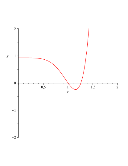
Figure 1: Plot of $\left(E_{0}^{W}\left[\partial\mathcal{M}\right]-E_{0}^{GS}\left[\partial\mathcal{M}\right]\right)_{1-loop}$ as a function of $x=r_{0}/r_{b}.$

The situation is better illustrated in Fig.$\left(\ref{Solfig}\right)$, where we immediately recognize that a tiny region exists where the ZPE is negative. This means that, in this range, the permanence of a wormhole is energetically favored with respect to a gravastar of the same mass $M$. The situation changes significantly if we avoid to fix the renormalization point with the choice of Eq.$\left(\ref{point}\right)$

Figure 2: Plot of $\left(E_{0}^{W}\left[\partial\mathcal{M}\right]-E_{0}^{GS}\left[\partial\mathcal{M}\right]\right)_{1-loop}$ as a function of $x=r_{0}/r_{b}$ and $y$.

This means that we are abandoning the continuity between the external and the internal region of the gravastar to one loop. In this case, Eq.$\left(\ref{DeltaEWGS}\right)$ becomes

$$\ln y\ \gtreqless\frac{4\ln 2-3x^{6}\ln x}{x^{6}-4},$$ (82)

where $x$ is given again by Eq.$\left(\ref{ratio}\right)$ and

$$y=\frac{3MG\sqrt{e}}{4r_{0}^{3}\mu_{0}^{2}}.$$ (83)

The behavior of the ZPE difference is shown in Fig.$\left(\ref{sol1}\right)$, where the equality of expression $\left(\ref{DeltaEWGS}\right)$ is reached when $\bar{y}=\bar{x}=0.4948$. It appears that below $\bar{y}$ and $\bar{x}$, the ZPE becomes negative denoting that the “ground state” between a wormhole and a gravastar is represented by a wormhole whose radius has to be smaller than the gravastar radius.

V Conclusions

In this paper we have considered one loop corrections to the $\mathcal{ADM}$ mass of a wormhole and a gravastar respectively. The motivation comes from the fact that a gravastar can represent an alternative to a black hole or a wormhole as regards the gravitational collapse. Nevertheless various problems of comparison arise because outside the gravastar radius, the metric is of the Schwarzschild type. If we adopt the energy point of view we find that, asymptotically, these configurations share the same $\mathcal{ADM}$ mass and therefore even in this case they are indistinguishable. However, since the gravastar has a different core with respect to the wormhole, a difference between them can emerge from a ZPE contribution. To this purpose we have computed an effective action to one loop, by looking at perturbations on the space-like hypersurface $\Sigma$. Since the perturbation involves only the spatial part of the metric, ghosts do not come into play for the energy contribution. Therefore, only the graviton is important to establish what happens to the ZPE. Note that every form of ZPE can be interpreted as an induced cosmological constant. In our case, this interpretation is very useful to apply standard regularization and renormalization procedures. In a sense, we can think that the ZPE induced by a wormhole or a gravastar contributes to a cosmological constant. On the other hand, we can think that the induced cosmological constant could be used to give a sorting to ZPE. It is interesting to note that, it is the double limit $\left(\ref{NonComm}\right)$ that denotes that something different appears in the throat proximity. This difference is principally caused by ZPE or Casimir energy which becomes so intense to create a thick barrier (“brick wall”) or a topology change (“gravastar”). Therefore, it is important to discover under what condition a wormhole persists or change into a gravastar or vice versa. It appears that a fundamental element to understand in which direction the geometry becomes relevant is in the radii ratio $\left(\ref{ratio}\right)$. Note that the comparison between the gravastar and the wormhole is done with the same mass $M$, as it should be. The other important parameter seems to be the renormalization point which, in this example, translates the presence or the absence of an energy gap between the external and the internal region of the gravastar. If one imposes the continuity of the ZPE through the gravastar radius, one meets a constraint on $\mu_{0}$ leading to the plot of Fig.$\left(\ref{Solfig}\right)$ showing that the region of permanence of the wormhole is very subtle. Indeed, from inequality $\left(\ref{ine}\right)$, outside the range $1<x<1.26$, the wormhole appears as an “excited state” with respect to the gravastar. In particular, one should note that the minimum for the ZPE difference appears for $x=1.152$ with a minimum value of $-0.244$. On the other hand, if one abandons the continuity condition of the gravastar ZPE and treats $\mu_{0}$ as a free parameter, one finds from Fig.$\left(\ref{sol1}\right)$ that the region of permanence of the wormhole is larger. Therefore we arrive at the conclusion that the permanence of a wormhole or a gravastar in their reciprocal comparison is strictly related to their size.

VI Acknowledgement

The author would like to thank R. Casadio, F.S.N. Lobo and D. Vassilevich for useful comments, discussions and hints.

Appendix A Disentangling the gauge modes

To explicitly make calculations, we need an orthogonal decomposition for $h_{\mu\nu}$ to disentangle gauge modes from physical deformations. To this purpose it is convenient to decompose $h_{\mu\nu}$ into a trace, longitudinal and transverse-traceless part in $D$ dimensionsMM1 ; Vassilevich ; Quad :

$$h_{\mu\nu}=\frac{1}{D}hg_{\mu\nu}+\left(L\xi\right)_{\mu\nu}+h_{\mu\nu}^{\bot},$$ (84)

where the operator $L$ maps $\xi_{\mu}$ into symmetric tracefree tensors

$$\left(L\xi\right)_{\mu\nu}=\nabla_{\mu}\xi_{\nu}+\nabla_{\nu}\xi_{\mu}-\frac{2}{D}g_{\mu\nu}\left(\nabla\cdot\xi\right)$$ (85)

and

$$g^{\mu\nu}h_{\mu\nu}^{\bot}=0,\qquad\nabla^{\mu}h_{\mu\nu}^{\bot}=0.$$ (86)

The decomposition $\left(\ref{dec}\right)$ is orthogonal with respect to the following inner product

$$\left\langle h,k\right\rangle:=\int_{\mathcal{M}}d^{D}x\sqrt{-g}G^{\mu\nu\rho\sigma}h_{\mu\nu}\left(x\right)k_{\rho\sigma}\left(x\right),$$ (87)

where

$$G^{\mu\nu\rho\sigma}=\frac{1}{2}(g^{\mu\rho}g^{\nu\sigma}+g^{\mu\sigma}g^{\nu\rho}+Cg^{\mu\nu}g^{\rho\sigma})$$ (88)

and $C$ is a constant. For the positivity of $G^{\mu\nu\rho\sigma}$ $C>-1/2$. The inverse metric is defined on cotangent space and it assumes the form

$$\left\langle p,q\right\rangle:=\int_{\mathcal{M}}d^{D}x\sqrt{-g}G_{\mu\nu\rho\sigma}p^{\mu\nu}\left(x\right)q^{\rho\sigma}\left(x\right),$$ (89)

so that

$$G^{\mu\nu\alpha\beta}G_{\alpha\beta\rho\sigma}=\frac{1}{2}\left(\delta_{\rho}^{\mu}\delta_{\sigma}^{\nu}+\delta_{\sigma}^{\mu}\delta_{\rho}^{\nu}\right).$$ (90)

Following Ref.Vassilevich , we observe that under the action of infinitesimal diffeomorphism generated by a vector field $\epsilon_{\mu}$, the components of $\left(\ref{dec}\right)$ transform as follows

$$\xi_{\mu}\longrightarrow\xi_{\mu}+\epsilon_{\mu},\qquad h\longrightarrow h+2\nabla^{\mu}\epsilon_{\mu},\qquad h_{\mu\nu}^{\bot}\longrightarrow h_{\mu\nu}^{\bot}.$$ (91)

We can fix the gauge freedom $\left(\ref{gauge}\right)$, by fixing

$$\xi_{\mu}=0.$$ (92)

If the manifold admits conformal Killing vectors, namely vectors annihilated by the operator $L$, one additional gauge condition involving the trace is necessary. Assume that such vectors are absent form the manifold. The Jacobian factor induced by the change of variable, namely $h_{\mu\nu}\rightarrow\left(h,\xi_{\mu},h_{\mu\nu}^{\bot}\right)$ is

$$J=\det_{V}\left(L^{\dagger}L\right)^{\frac{1}{2}},$$ (93)

where the determinant is calculated in the space of vector fields excluding conformal Killing vectors. Using the definition $\left(\ref{Lapl}\right)$, the operator acting on vector fields is

$$\left(L^{\dagger}L\right)_{\mu}^{\nu}=-2\left(-\bigtriangleup\delta_{\mu}^{\nu}+\left(1-\frac{2}{D}\right)\nabla_{\mu}\nabla^{\nu}+R_{\mu}^{\nu}\right).$$ (94)

We can write decomposition $\left(\ref{dec}\right)$ in the following way

$$h_{\mu\nu}=\left(\sigma+2\nabla\cdot\xi\right)\frac{g_{\mu\nu}}{D}+\left(L\xi\right)_{\mu\nu}+h_{\mu\nu}^{\bot},$$ (95)

The change of variables $h\rightarrow\sigma$ does not introduce any additional Jacobian factor, then the path integral measure separates into

$$\mathcal{D}h_{\mu\nu}=\det_{V}\left(L^{\dagger}L\right)^{\frac{1}{2}}\mathcal{D}h^{\bot}\mathcal{D}\xi\mathcal{D}\sigma$$ (96)

and the quadratic part of the action $\left(\ref{S24d}\right)$ becomes

$$S^{\left(2\right)}=\frac{1}{2\kappa}\int_{\mathcal{M}}d^{4}x\sqrt{-g}\left[-\frac{1}{4}h^{\bot,\mu\nu}\left(\bigtriangleup_{L\!}\!{}h\right)_{\mu\nu}^{\bot}+\frac{3}{32}\sigma\bigtriangleup\!{}\sigma\right].$$ (97)

The path integral can be written in terms of functional determinants of transverse-traceless tensor fields (indicated by T), vector fields (indicated by V) and scalar fields (indicated by S):

$$Z=\det_{T}\left(\bigtriangleup_{L\!}\right)^{-\frac{1}{2}}\det_{V}\left(L^{\dagger}L\right)^{\frac{1}{2}}\det_{S}\left(-\bigtriangleup\right)^{-\frac{1}{2}}.$$ (98)

The determinant over vector fields is the analogue of the Faddeev-Popov determinant. We can further decompose it by introducing a Hodge decomposition

$$\xi=d\psi+\xi^{H}+\delta\omega=\xi^{||}+\xi^{H}+\xi^{\bot},$$ (99)

where $\psi$ is a zero-form, $\xi^{H}$ is a harmonic one-form and $\omega$ is a two-form. Excluding the presence of harmonic vectors $\xi^{H}$, we find that the operator $\left(\ref{LLVec}\right)$ separates into

$$\left(L^{\dagger}L\xi\right)_{\mu}=2\left(\bigtriangleup\xi_{\mu}^{\bot}-R_{\mu}^{\nu}\xi_{\mu}^{\bot}\right)+2\left(\bigtriangleup\xi_{\mu}^{||}-\left(1-\frac{2}{D}\right)\nabla_{\mu}\nabla^{\nu}\xi_{\nu}^{||}-R_{\mu}^{\nu}\xi_{\nu}^{||}\right)$$ (100)

and using the equations of motion on shell $R_{\mu\nu}=0$, we get for the Jacobian

$$\det_{V}\left(L^{\dagger}L\right)^{\frac{1}{2}}=\det_{V^{\bot}}\left(\bigtriangleup\right)^{\frac{1}{2}}\det_{V^{||}}\left(\bigtriangleup\right)^{\frac{1}{2}}$$ (101)

and the one loop effective action simplifies

$$\Gamma_{1-loop}=\frac{i}{2}\left[Tr\ln\bigtriangleup_{L\!}^{\bot}\!-Tr\ln\triangle_{V^{\bot}}\right]=\frac{i}{2}\int_{\mathcal{M}}d^{4}x\sqrt{-g}\left[\int\frac{d^{4}k}{\left(2\pi\right)^{4}}\ln\lambda_{TT}^{2}-\int\frac{d^{4}k}{\left(2\pi\right)^{4}}\ln\lambda_{V^{\bot}}^{2}\right],$$ (102)

where $\lambda_{TT}^{2}$ and $\lambda_{V^{\bot}}^{2}$ are the eigenvalues of the Lichnerowicz operator for TT tensors and the transverse vector operator respectively. Before going on, we need to precise a point concerning the computation of a functional determinant. Generally speaking the functional determinant of a given differential operator $O$ can be represented by

$$\det O=\exp\left(Tr\ln O\right).$$ (103)

However within the zeta function regularization, it is no longer true that

$$\det AB=\det A\det B,$$ (104)

where $A$ and $B$ are two elliptic operators. In general, one has

$$\det AB=\exp a\left(A,B\right)\det A\det B.$$ (105)

where $a\left(A,B\right)$ is a local functional called multiplicative anomaly. As pointed out in Ref.EVZ , one can assume the multiplicative anomaly to be trivial, namely $a\left(A,B\right)=0$. This is justified by the fact that to one loop approximation a non-trivial multiplicative anomaly may be absorbed into the renormalization ambiguity.

A.1 Evaluating $\det_{V}\left(L^{\dagger}L\right)$ in $3$ dimensions

In Eqs.$\left(\ref{dec}\right)$, $\left(\ref{gaugev}\right)$ and $\left(\ref{LL4D}\right)$, we have simply to put $D=3$. In addition, we have to remind that, in this case the Ricci tensor is not vanishing. If $\xi_{a}$ is further decomposed into a transverse part $\xi_{a}^{T}$ with $\nabla^{a}\xi_{a}^{T}=0$ and a longitudinal part $\xi_{a}^{\parallel}$ with $\xi_{a}^{\parallel}=$ $\nabla_{a}\psi$, then the orthogonal decomposition reduces to

$$\left\langle L\xi,L\xi\right\rangle:=\int_{\mathcal{M}}d^{3}x\sqrt{-g}\left(L\xi\right)^{ij}\left(L\xi\right)_{ij}$$ (106)

$$=\int_{\mathcal{M}}d^{D}x\sqrt{-g}\left[2\xi_{i}^{T}\bigtriangleup_{V}^{ij}\xi_{j}^{T}-4\xi_{i}^{T}R^{ij}\nabla_{j}\psi-4\psi\left(\frac{2}{3}\bigtriangleup^{2}+\nabla_{i}R^{ij}\nabla_{j}\right)\psi\right],$$ (107)

with

$$\bigtriangleup_{V}^{ij}=\bigtriangleup g^{ij}-R^{ij}.$$ (108)

The decomposition $\left(\ref{hh}\right)$ is orthogonal up to the $\xi_{j}^{T}-\psi$-mixed terms. If we try to compute the related Jacobian induced by the vector-scalar part in Eq.$\left(\ref{hh}\right)$, we obtain

$$\int\mathcal{D}\xi\exp\left[-\frac{i}{2}\left\langle L\xi,L\xi\right\rangle\right]=$$

$$J_{1}\int\mathcal{D}\xi\mathcal{D}\psi\exp\left[-\frac{i}{2}\int_{\mathcal{M}}d^{D}x\sqrt{-g}\left\{\left[\xi_{i}^{T},\psi\right]M^{\left(i,j\right)}\left[\xi_{j}^{T},\psi\right]^{T}\right\}\right]=1.$$ (109)

In terms of the functional determinant

$$J_{1}=\left(\det\nolimits_{\xi^{T},\psi}\left[M^{\left(i,j\right)}\right]\right)^{\frac{1}{2}},$$ (110)

where $M^{\left(i,j\right)}$ a $\left(3+1\right)\times\left(3+1\right)$-matrix differential operator whose first 3 columns act on transverse spin one field $\xi_{j}^{T}$ and whose last columns acts on the spin zero field $\psi$. From Eq.$\left(\ref{hh}\right)$, the corresponding matrix can be read off,

$$M^{\left(i,j\right)}=\begin{bmatrix}2\bigtriangleup_{V}^{T,ij}&-4R^{ij}\nabla_{j}\\ 0&-2\left(\frac{2}{3}\bigtriangleup^{2}+\nabla_{i}R^{ij}\nabla_{j}\right)\end{bmatrix}.$$ (111)

Thus Eq.$\left(\ref{dLL4D}\right)$ becomes

$$\left(\det\nolimits_{\xi^{T},\psi}\left[M^{\left(i,j\right)}\right]\right)^{\frac{1}{2}}=\left(\det\bigtriangleup_{V}^{T}\right)^{\frac{1}{2}}\left(\det\left[\frac{2}{3}\bigtriangleup^{2}+\nabla_{i}R^{ij}\nabla_{j}\right]\right)^{\frac{1}{2}}.$$ (112)

The presence of the Ricci tensor in the scalar term of Eq.$\left(\ref{detM}\right)$ is an artifact of the foliation, because in 4 dimensions it disappears. By means of the contracted Bianchi identities $\nabla_{i}R^{ij}=\nabla^{j}R/2$, we can simplify somewhat the expression of the scalar term of Eq.$\left(\ref{detM}\right)$

$$\frac{2}{3}\bigtriangleup^{2}+\nabla_{i}R^{ij}\nabla_{j}=\frac{2}{3}\bigtriangleup^{2}+\frac{1}{2}\nabla^{j}R\nabla_{j}+R^{ij}\nabla_{i}\nabla_{j}.$$ (113)

The determinant of the operator in Eq.$\left(\ref{JS}\right)$ can be cast into the following form

$$\det\left(\frac{2}{3}\bigtriangleup^{2}+R^{ij}\nabla_{i}\nabla_{j}\right)^{\frac{1}{2}}=\exp\frac{1}{2}Tr\ln\left(\frac{2}{3}\bigtriangleup^{2}+R^{ij}\nabla_{i}\nabla_{j}\right)$$

$$=\exp\frac{1}{2}Tr\ln\left[\left(\frac{2}{3}\bigtriangleup^{2}\right)\left(\mathbf{1}\mathbb{+}\left(\frac{2}{3}\bigtriangleup^{2}\right)^{-1}+R^{ij}\nabla_{i}\nabla_{j}\right)\right]$$

$$=\exp\frac{1}{2}Tr\left[\ln\left(\frac{2}{3}\bigtriangleup^{2}\right)+\ln\left(\mathbf{1}\mathbb{+}\left(\frac{2}{3}\bigtriangleup^{2}\right)^{-1}R^{ij}\nabla_{i}\nabla_{j}\right)\right].$$ (114)

The second term is a correction to the principal part and will not be considered in the W.K.B. method. The main part of the operator reduces to

$$\det\left(\frac{2}{3}\bigtriangleup^{2}\right)^{\frac{1}{2}}=\left(\det\bigtriangleup\right)^{\frac{1}{2}},$$ (115)

where we have absorbed the constant factor into the definition of the determinant and we have redefined the scalar wave function in such a way to absorb the operator $\bigtriangleup$. To summarize, Eq.$\left(\ref{dLL4D}\right)$ in 3 dimensions becomes

$$\det_{V}\left(L^{\dagger}L\right)^{\frac{1}{2}}=\left(\det\bigtriangleup_{V}^{T}\right)^{\frac{1}{2}}\left(\det\bigtriangleup\right)^{\frac{1}{2}}.$$ (116)

With the help of the functional determinant in Eq.$\left(\ref{dLL3D}\right)$, the one loop effective action can be written as

$$\Gamma_{1-loop}=\left(\det\bigtriangleup_{V}^{T}\right)^{\frac{1}{2}}\det\left(\bigtriangleup\right)^{\frac{1}{2}}\left(\det\tilde{\bigtriangleup}_{L\!}\right)^{-\frac{1}{2}}\left(\det\tilde{\bigtriangleup}_{\sigma}\right)^{-\frac{1}{2}}.$$ (117)

One can observe that the scalar determinants should cancel each other except for three subtleties. First the sign of the operator $\tilde{\bigtriangleup}\sigma$ in $\left(\ref{M scalar}\right)$ appears to be different from that in the Jacobian, second the integration leading to $\left(\ref{detM}\right)$ excludes zero modes not included in the Jacobian, so any cancellation will not be complete. This also happens in the full covariant computation. Last but not least, the cancellation should be done after integration over the time part in the determinant of the operator.

Appendix B The Lichnerowicz operator for TT tensors

Our starting point is the expression $\left(\ref{quadr}\right)$ and the metric $\left(\ref{metric}\right)$. For the benefit of the reader, we recall the representation of the operator $O$

$$O^{ikjl}=\bigtriangleup_{L}^{ikjl}-4R^{il}g^{kj}+Rg^{ik}g^{jl}+\frac{\partial^{2}}{\partial t^{2}}g^{ik}g^{jl}$$ (118)

and we simplify the expression of the Riemann tensor in $3$ dimensions

$$R_{ikjl}=g_{ij}R_{kl}-g_{il}R_{kj}-g_{kj}R_{il}+g_{kl}R_{ij}-\frac{R}{2}\left(g_{ij}g_{kl}-g_{il}g_{kj}\right).$$ (119)

Then, the operator $O^{ikjl}$ becomes

$$-\nabla^{a}\nabla_{a}g^{ik}g^{jl}+\frac{\partial^{2}}{\partial t^{2}}g^{ik}g^{jl}-2\left(g^{ij}R^{kl}-g^{il}R^{kj}-g^{kj}R^{il}+g^{kl}R^{ij}\right)+R\left(g^{ij}g^{kl}-g^{il}g^{kj}\right)$$

$$+R^{ik}g^{jl}+R^{jk}g^{il}-4R^{il}g^{kj}+Rg^{ik}g^{jl}=-\nabla^{a}\nabla_{a}g^{ik}g^{jl}+\frac{\partial^{2}}{\partial t^{2}}g^{ik}g^{jl}$$

$$-2\left(g^{ij}R^{kl}+g^{kl}R^{ij}\right)+R\left(g^{ij}g^{kl}-g^{il}g^{kj}\right)+R^{ik}g^{jl}+3R^{jk}g^{il}-2R^{il}g^{kj}+Rg^{ik}g^{jl}.$$ (120)

When we fix our attention on TT tensors, we obtain a further reduction

$$O^{ikjl}=-\nabla^{a}\nabla_{a}g^{ik}g^{jl}+\frac{1}{N^{2}}\frac{\partial^{2}}{\partial t^{2}}g^{ik}g^{jl}+2R^{il}g^{kj}.$$ (121)

Thus the related eigenvalue equation is

$$-\left(\triangle_{2}h^{TT}\right)_{i}^{j}+\frac{1}{N^{2}}\frac{\partial^{2}}{\partial t^{2}}h_{i}^{j}=\lambda^{2}h_{i}^{j}$$ (122)

where

$$\left(\triangle_{2}h^{TT}\right)_{i}^{j}:=\left(-\triangle_{T}h^{TT}\right)_{i}^{j}+2\left(Rh^{TT}\right)_{i}^{j}$$ (123)

and

$$-\left(\triangle_{T}h^{TT}\right)_{i}^{j}=-\triangle_{S}\left(h^{TT}\right)_{i}^{j}+\frac{6}{r^{2}}\left(1-\frac{b\left(r\right)}{r}\right)\left(h^{TT}\right)_{i}^{j}.$$ (124)

$\triangle_{S}$ is the scalar curved Laplacian computed on the background of metric $\left(\ref{metric}\right)$, whose form is

$$\triangle_{S}=\left(1-\frac{b\left(r\right)}{r}\right)\frac{d^{2}}{dr^{2}}+\left(\frac{4r-b^{\prime}\left(r\right)r-3b\left(r\right)}{2r^{2}}\right)\frac{d}{dr}-\frac{L^{2}}{r^{2}}$$ (125)

and $R_{j\text{ }}^{a}$ is the mixed Ricci tensor whose components are:

$$R_{i}^{a}=\left\{\frac{b^{\prime}\left(r\right)}{r^{2}}-\frac{b\left(r\right)}{r^{3}},\frac{b^{\prime}\left(r\right)}{2r^{2}}+\frac{b\left(r\right)}{2r^{3}},\frac{b^{\prime}\left(r\right)}{2r^{2}}+\frac{b\left(r\right)}{2r^{3}}\right\}.$$ (126)

We will follow Regge and Wheeler in analyzing the equation as modes of definite frequency, angular momentum and parityRW . In particular, our choice for the three-dimensional gravitational perturbation is represented by its even-parity form

$$h_{ij}^{even}\left(t,r,\vartheta,\phi\right)=diag\left[H\left(r\right)\left(1-\frac{b\left(r\right)}{r}\right)^{-1},r^{2}K\left(r\right),r^{2}\sin^{2}\vartheta K\left(r\right)\right]Y_{lm}\left(\vartheta,\phi\right)F\left(t\right).$$ (127)

For a generic value of the angular momentum $L$ representation $\left(\ref{pert}\right)$, together with Eqs.$\left(\ref{tlap},\ref{p31}\right)$ leads to the following system of PDE’s

$$\left\{\begin{array}[c]{c}\left(-\triangle_{l}+2\left(\frac{b^{\prime}\left(r\right)}{r^{2}}-\frac{b\left(r\right)}{r^{3}}\right)+\frac{\partial^{2}}{\partial t^{2}}\right)H\left(r\right)F\left(t\right)=\lambda_{1,l}^{2}H\left(r\right)F\left(t\right)\\ \\ \left(-\triangle_{l}+2\left(\frac{b^{\prime}\left(r\right)}{2r^{2}}+\frac{b\left(r\right)}{2r^{3}}\right)+\frac{\partial^{2}}{\partial t^{2}}\right)K\left(r\right)F\left(t\right)=\lambda_{2,l}^{2}K\left(r\right)F\left(t\right)\end{array}\right.,$$ (128)

where $\triangle_{l}$ is

$$\triangle_{l}=\left(1-\frac{b\left(r\right)}{r}\right)\frac{d^{2}}{dr^{2}}+\left(\frac{4r-b^{\prime}\left(r\right)r-3b\left(r\right)}{2r^{2}}\right)\frac{d}{dr}-\frac{l\left(l+1\right)}{r^{2}}-\frac{6}{r^{2}}\left(1-\frac{b\left(r\right)}{r}\right).$$ (129)

The action of $\triangle_{l}$ on the reduced fields

$$H\left(r\right)=\frac{f_{1}\left(r\right)}{r};\qquad K\left(r\right)=\frac{f_{2}\left(r\right)}{r}$$ (130)

is

$$\triangle_{l}\left(\frac{f_{1,2}\left(r\right)}{r}\right)=\frac{1}{r}\left\{\left(1-\frac{b\left(r\right)}{r}\right)\frac{d^{2}}{dr^{2}}+\frac{1}{r}\left[-2\left(1-\frac{b\left(r\right)}{r}\right)+\left(\frac{4r-b^{\prime}\left(r\right)r-3b\left(r\right)}{2r}\right)\right]\frac{d}{dr}\right.$$

$$\left.+\frac{1}{r^{2}}\left[2\left(1-\frac{b\left(r\right)}{r}\right)-\left(\frac{4r-b^{\prime}\left(r\right)r-3b\left(r\right)}{2r}\right)\right]-\frac{l\left(l+1\right)}{r^{2}}-\frac{6}{r^{2}}\left(1-\frac{b\left(r\right)}{r}\right)\right\}f_{1,2}\left(r\right)$$

$$=\frac{1}{r}\left\{\left(1-\frac{b\left(r\right)}{r}\right)\frac{d^{2}}{dr^{2}}+\frac{1}{r}\left[-\frac{b^{\prime}\left(r\right)}{2}+\frac{b\left(r\right)}{2r}\right]\frac{d}{dr}+\frac{1}{r^{2}}\left[\frac{b^{\prime}\left(r\right)}{2}-\frac{b\left(r\right)}{2r}\right]-\frac{l\left(l+1\right)}{r^{2}}-\frac{6}{r^{2}}\left(1-\frac{b\left(r\right)}{r}\right)\right\}f_{1,2}\left(r\right)$$ (131)

and using the proper geodesic distance from the throat

$$dx=\pm\frac{dr}{\sqrt{1-\frac{b\left(r\right)}{r}}},$$ (132)

we get

$$=\frac{1}{r}\left\{\frac{d^{2}}{dx^{2}}+\frac{1}{r^{2}}\left[\frac{b^{\prime}\left(r\right)}{2}-\frac{b\left(r\right)}{2r}\right]-\frac{l\left(l+1\right)}{r^{2}}-\frac{6}{r^{2}}\left(1-\frac{b\left(r\right)}{r}\right)\right\}f_{1,2}\left(r\right),$$ (133)

where $r\equiv r\left(x\right)$. Thus, the system $\left(\ref{p33}\right)$ becomes

$$\left\{\begin{array}[c]{c}\left[-\frac{d^{2}}{dx^{2}}+\frac{\partial^{2}}{\partial t^{2}}+V_{1}\left(r\right)\right]f_{1}\left(x\right)F\left(t\right)=\lambda_{1,l}^{2}f_{1}\left(x\right)F\left(t\right)\\ \\ \left[-\frac{d^{2}}{dx^{2}}+\frac{\partial^{2}}{\partial t^{2}}+V_{2}\left(r\right)\right]f_{2}\left(x\right)F\left(t\right)=\lambda_{2,l}^{2}f_{2}\left(x\right)F\left(t\right)\end{array}\right.$$ (134)

with

$$\left\{\begin{array}[c]{c}V_{1}\left(r\right)=\frac{l\left(l+1\right)}{r^{2}}+U_{1}\left(r\right)\\ \\ V_{2}\left(r\right)=\frac{l\left(l+1\right)}{r^{2}}+U_{2}\left(r\right)\end{array}\right.,$$ (135)

and

$$\left\{\begin{array}[c]{c}U_{1}\left(r\right)=\frac{6}{r^{2}}\left(1-\frac{b\left(r\right)}{r}\right)+\left[\frac{3}{2r^{2}}b^{\prime}\left(r\right)-\frac{3}{2r^{3}}b\left(r\right)\right]=m_{1}^{2}\left(r\right)\\ U_{2}\left(r\right)=\frac{6}{r^{2}}\left(1-\frac{b\left(r\right)}{r}\right)+\left[\frac{1}{2r^{2}}b^{\prime}\left(r\right)+\frac{3}{2r^{3}}b\left(r\right)\right]=m_{2}^{2}\left(r\right)\end{array}\right.,$$ (136)

where we have defined two effective masses dependent on $r$. Now let us consider the following state

$$\left\langle t,r,\theta,\phi|\omega,k.l.m\right\rangle=\frac{1}{r}f_{i}\left(x\right)Y_{lm}\left(\vartheta,\phi\right)\exp\left(-i\omega t\right),$$ (137)

then the system $\left(\ref{F p33}\right)$ becomes

$$\left\{\begin{array}[c]{c}\left[-\frac{d^{2}}{dx^{2}}-\omega^{2}+V_{1}\left(r\right)\right]f_{1}\left(x\right)=\tilde{\lambda}_{1,l}^{2}f_{1}\left(x\right)\\ \\ \left[-\frac{d^{2}}{dx^{2}}-\omega^{2}+V_{2}\left(r\right)\right]f_{2}\left(x\right)=\tilde{\lambda}_{2,l}^{2}f_{2}\left(x\right)\end{array}\right..$$ (138)

References

References

• (1) R. M. Wald, Living Rev. Rel. 4, 6 (2001); ArXiv:gr-qc/9912119.
• (2) P.O. Mazur and E. Mottola, “Gravitational Condensate Stars: An Alternative to Black Holes”, ArXiv: gr-qc/0109035; Proc. Nat. Acad. Sci. 101, 9545 (2004), ArXiv:gr-qc/0407075.
• (3) A. DeBenedictis, D. Horvat, S. Ilijic, S. Kloster and K.S. Viswanathan Class.Quant.Grav. 23 2303 (2006); ArXiv:gr-qc/0511097.
• (4) I. G. Dymnikova, Class. Quant. Grav. 19 725 (2002); ArXiv:gr-qc/0112052. I. G. Dymnikova, Phys. Lett. B 472 33 (2000); ArXiv:gr-qc/9912116. I. G. Dymnikova, “Variable cosmological contrast: Geometry and physics.” ArXiv: gr-qc/0010016. I. G. Dymnikova, Gen. Rel. Grav. 24 235 (1992).
• (5) R. Arnowitt, S. Deser, and C. W. Misner, in Gravitation: An Introduction to Current Research, edited by L. Witten (John Wiley & Sons, Inc., New York, 1962). ArXiv:gr-qc/0405109.
• (6) T. Harko, Z. Kovacs and F.S.N. Lobo, Class.Quant.Grav. 26 215006 (2009); ArXiv:0905.1355 [gr-qc].
• (7) C. B. M. H. Chirenti and L. Rezzolla, Class.Quant.Grav. 24 4191 (2007); ArXiv:0706.1513 [gr-qc].
• (8) V. Cardoso, P. Pani, M. Cadoni and M. Cavaglià, Phys.Rev. D 77, 124044 (2008); ArXiv:0709.0532 [gr-qc].
• (9) C. B. M. H. Chirenti and L. Rezzolla, Phys.Rev. D 78, 084011 (2008); ArXiv:0808.4080 [gr-qc].
• (10) G.W. Gibbons and M.J. Perry, Nucl.Phys. B 146, 90 (1978).
• (11) S.M. Christensen and M.J. Duff, Nucl.Phys. B 170, 480 (1980).
• (12) P. O. Mazur and E. Mottola, Nucl.Phys. B 341, 187 (1990).
• (13) For technical details, see R. Garattini, TSPU Vestnik 44 N7, 72 (2004); gr-qc/0409016. R.Garattini, Casimir Energy, the Cosmological Constant and Massive Gravitons. gr-qc/0510062. R.Garattini, J. Phys. A 39, 6393 (2006); gr-qc/0510061. R. Garattini, J.Phys.Conf.Ser. 33, 215 (2006); gr-qc/0510062. S. Capozziello and R. Garattini, Class.Quant.Grav. 24, 1627 (2007); gr-qc/0702075.
• (14) M.Yu.Kalmykov and P.I.Pronin, Gen.Rel.Grav. 27, 873 (1995); hep-th/9412177v2.
• (15) P.A. Griffin and D.A. Kosower, Phys.Lett. B 233, 295 (1989).
• (16) I.O. Cherednikov, Acta Physica Slovaca, 52, (2002), 221. I.O. Cherednikov, Acta Phys.Polon. B 35, 1607 (2004). M. Bordag, U. Mohideen and V.M. Mostepanenko, Phys.Rep. 353, 1 (2001).
• (17) D. V. Ahluwalia, Int.J.Mod.Phys. D 8, 651 (1999). ArXiv: astro-ph/9909192.
• (18) N.K. Nielsen and P. Olesen, Nucl.Phys. B 144, 376 (1978).
• (19) G. ’t Hooft, Nucl. Phys. B 256, 727 (1985).
• (20) A.DeBenedictis, R. Garattini and F. S.N. Lobo, Phys.Rev. D 78, 104003 (2008); ArXiv:0808.0839 [gr-qc].
• (21) S. W. Hawking and G. T. Horowitz, Class.Quant.Grav. 13 1487, (1996); ArXiv:gr-qc/9501014.
• (22) D.V. Vassilevich, Int. J. Mod. Phys. A 8, 1637 (1993).
• (23) M. Berger and D. Ebin, J.Diff.Geom. 3, 379 (1969). J. W. York Jr., J.Math.Phys., 14, 4 (1973); Ann. Inst. Henri Poincaré A 21, 319 (1974).
• (24) E. Elizalde, L. Vanzo and S. Zerbini, Commun.Math.Phys. 194, 613 (1998), hep-th/9701060; E. Elizalde, A. Filippi, L. Vanzo and S. Zerbini, Phys.Rev. D 57, 7430 (1998), hep-th/9710171.
• (25) T. Regge and J. A. Wheeler, Phys.Rev. 108, 1063 (1957).