The end of the white dwarf cooling sequence in M 67

In this paper, we present for the first time a proper-motion-selected white dwarf (WD) sample of the old Galactic open cluster M 67, down to the bottom of the WD cooling sequence (CS). The color-magnitude diagram is based on data collected with the LBC-Blue camera at the prime focus of LBT. As first epoch data, we used CFHT-archive images collected 10 years before LBC data. We measured proper motions of all the identified sources. Proper motions are then used to separate foreground and background objects from the cluster stars, including WDs. Finally, the field-object cleaned WD CS in the $V$ vs. $B-I$ color-magnitude diagram is compared with the models. We confirm that the age derived from the location of the bottom of the WD CS is consistent with the turn off age.

1 Introduction

The white dwarf (WD) cooling sequence (CS) lies in one of the most unexplored parts of the color-magnitude diagram (CMD) of star clusters. In a recent deep photometric investigation of the metal rich open cluster NGC 6791, Bedin et al. (2005; 2008a,b) discovered an unexpectedly bright peak in its WD luminosity function (LF). This result raises questions about our understanding of the physical processes that rule the formation of WDs and their cooling phases. It is clear that, in order to improve our current understanding of WDs, in particular at high metallicities, we need to fill the age-metallicity parameter space of stellar clusters with new data.

Unfortunately, most of the metal-rich old open clusters for which the end of the WD CS is potentially reachable are relatively sparse. Because of this, the limited field of view of Hubble Space Telescope (HST) cameras allows us to cover only a small fraction of a single cluster, which implies that a very limited number of WDs can be observed.

The dispersion of the cluster stars over a large field has the additional inconvenience of a strong contamination of all of the evolutionary sequences in the CMD by foreground/background objects. The two wide-field imagers (WFIs) at the two prime foci of LBT provide us with a unique opportunity to overcome the field size problem. Moreover, the availability of multi-epoch imaging allows us to measure proper motions, thus alleviating the issue of field contamination.

Note that, although (in principle) it would be possible to entirely map an open cluster as large as M 67 with HST, during its 19 years of activity these kind of projects have never been approved. For reference, in the case of M 67 it would be necessary a minimum of $\sim$40 orbits —per epoch— to map the inner $\sim$20$\times$20 arcmin², taking into account for: dump-buffer overheads, intra-orbit pointing limitations, and the necessity to have multiple exposures with large dithers. For practical reasons, for nearby clusters, ground-based telescopes with wide field of view (FoV) are more appropriate to achieve this purpose, and at much cheaper costs.

In this paper, we present a pioneering work on this subject. For the first time, we used wide-field astrometry and deep photometry to obtain a pure sample of WDs in the open cluster M 67 [($\alpha,\delta)$_J2000.0=(8^h51^m$23\aas@@fstack{s}3$,$+$11^∘49^′02${\arcsec}$), Yadav et al. (2008)]. First epoch photometry from a WFIs is available only from a 4m class telescope, and our LBC@LBT images were not acquired in optimal conditions. Yet we have been able to reach the end of the WD CS, remove field objects by using proper motions, and demonstrate the potentiality of a wide field imager (particularly if mounted on a 8m class telescope) for the WD study.

A WD study of M 67 was already published by Richer et al. (richer98 (1998), hereafter R98) using the same data set that we use here as first epoch images. R98 could not directly see the end of the WD CS, because of the strong contamination by background field galaxies, but they could infer its location by a statistical analysis of star counts around the region in the CMD where the WDs are expected to be. The great news presented in this paper is that we can now remove most of the field objects and present a clean WD CS down to its bottom.

2 Observations

We used as first-epoch data a set of images collected on January 10–13, 1997 at the CFHT 3.6m telescope. This data set (a sub-set of those used also by R98) consists of 15$\times$1200 s $V$-band, and 11$\times$1200 s $I$-band images, obtained with the UH8K camera (8 CCDs, 2K$\times$4K pixels each, in a 4$\times$2 array). Two chips (# 2 and 4) of this camera are seriously affected by charge transfer inefficiency. As a consequence, the FoV suitable for high precision measurements is reduced to only six chips (for a total sky coverage of $\sim$400 arcmin²). [We will see that none of our WDs fall within those detectors.] The median seeing is $1\aas@@fstack{\prime\prime}0$.

Table 1: Log of M 67 data used in this work.

Filter	#Images$\times$Exp. time	Airmass	Seeing
	$(s)$	$(\sec z)$	(arcsec)
UH8k@CFHT (First Epoch: 10–13 Jan 1997)
$V_{\rm Johnson}$	$15\times 1200$	1.02–1.50	0.74–1.37
$I_{\rm Johnson}$	$11\times 1200$	1.02–1.70	0.75–1.26
LBC@LBT (Second epoch: 18 Feb–16 Mar 2007)
$B_{\rm Bessel}$	$56\times 180$	1.07–1.14	0.79–1.88
$V_{\rm Bessel}$	$1\times 15$, $25\times 100$	1.07–1.10	0.68–1.26
	$17\times 110$, $1\times 330$	1.07–1.12	0.62–1.31

The second epoch data, collected between February 16 and March 18, 2007, consists of 56$\times$180 s $B$-band, and 1$\times$15 s, 25$\times$100 s, 17$\times$110 s, 1$\times$330 s $V$-band images, obtained with the LBC-blue camera (4 CCDs, 2K$\times$4.5K pixels each, 3 aligned longside, one rotated 90^∘ on top of them, FoV of $\sim$24^′$\times$25^′, see Giallongo et al. giallongo08 (2008)). This data set is not optimal: the original project consists in a set of 25$\times$180s $B$ and 25$\times$110s $V$ images for science purposes, plus 25$\times$100s $V$ images to solve for the geometric distortion (hereafter GD). All 100 s $V$ images have anomalously high background ($\sim$20 000 digital numbers (DNs) instead of an expected $\sim$3000). The median seeing is $1\aas@@fstack{\prime\prime}0$ for the $V$ filter, and $1\aas@@fstack{\prime\prime}3$ for the $B$ one. See Table 1 for the complete log of observations.

3 Measurements and Selections

We successfully exported our data reduction software developed for HST images (Anderson et al. anderson08 (2008)), adapting it to the case of ground-based WFIs. Below, we briefly describe our 3-step procedure, used on both LBC and UH8K data sets. Further details on data reduction and calibration procedures are presented in two companion papers (Bellini & Bedin submitted, Bellini et al. in preparation).

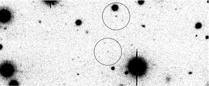
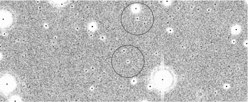
Figure 1: (Top:) A region of a LBT $V$ image (110 s exposure, seeing $\sim$1$\arcsec$, North is up, East is to the left) in which two WDs are present, highlighted by open circles (the southern-most one is also the faintest WD in our sample). (Bottom): the same region as seen on our 3$\times$3 overbinned peak map. The FoV is $\sim$170$\arcsec$$\times$70$\arcsec$. See text for details.

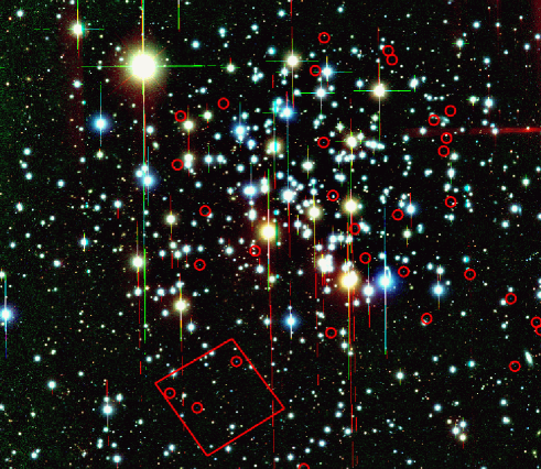
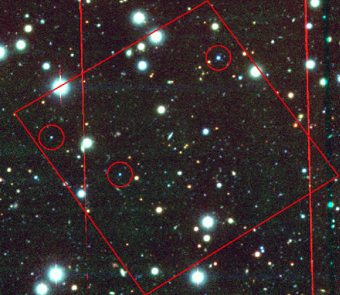
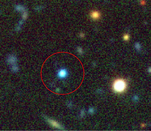
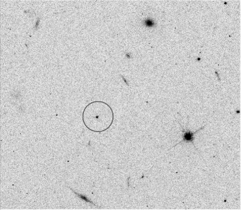
Figure 2: (Top left): The central $\sim$20$\times$17 arcmin² region of our stacked trichromatic image from $BV$-LBT and $I$-CFHT frames. North is up, East is to the left. Red circles highlight the proper-motion selected WDs within the region. The red trapezoid indicates an HST ACS/WFC field from the archive (combining 1$\times$400 s and 1$\times$568 s images in filter F775W; GO-9984). (Top right): An enlargement of the area in common with the ACS/WFC field. (Bottom left): Zoom-in around the southern-most WD within the ACS/WFC field. The area is $\sim$40$\arcsec$ wide. The circle has a radius of 25 pixels. (Bottom right): The same portion of the field, but as seen in the ACS/WFC stacked image.

3.1 First step

We used the software described in Anderson et al. (anderson06 (2006)) to obtain spatially varying empirical PSFs (in an array of 3$\times$7 each chip for LBC, and in an array of 3$\times$5 for each UH8K chip), with which we measured star positions and fluxes in each single chip of each individual exposure. We then corrected LBC raw positions for GD according to Bellini & Bedin (submitted). In a nutshell, we modeled the GD with a third-order polynomial, for each LBC chip independently. For each $i$-star in each $k$-chip, the distortion corrected position $(x_{i,k}^{\rm corr},y_{i,k}^{\rm corr})$ is obtained as the observed position $(x_{i,k},y_{i,k})$ plus the distortion correction $(\delta x_{i,k},\delta y_{i,k})$:

$$\left\{\begin{array}[]{rcl}x_{i,k}^{\rm corr}&\!\!=\!\!&x_{i,k}+\delta x_{i,k}(\tilde{x}_{i,k},\tilde{y}_{i,k})\\ y_{i,k}^{\rm corr}&\!\!=\!\!&y_{i,k}+\delta y_{i,k}(\tilde{x}_{i,k},\tilde{y}_{i,k}),\\ \end{array}\right.$$

where $\tilde{x}_{i,k}$ and $\tilde{y}_{i,k}$ are normalized positions with respect to the center $(x_{\circ},y_{\circ})_{k}$ of the $k$-chip [assumed to be the pixel (1025,2305) for chips # 1 to 3, and (2305,1025) for chip # 4], and $(\delta x_{i,k},\delta y_{i,k})$ are given as:

$$\left\{\begin{array}[]{rcl}\displaystyle\!\!\delta x&\!\!=\!\!&a_{1}\tilde{x}\!+\!a_{2}\tilde{y}\!+\!a_{3}\tilde{x}^{2}\!+\!a_{4}\tilde{x}\tilde{y}\!+\!a_{5}\tilde{y}^{2}\!+\!a_{6}\tilde{x}^{3}\!+\!a_{7}\tilde{x}^{2}\tilde{y}\!+\!a_{8}\tilde{x}\tilde{y}^{2}\!+\!a_{9}\tilde{y}^{3}\\ \displaystyle\!\!\delta y&\!\!=\!\!&b_{1}\tilde{x}\!+\!b_{2}\tilde{y}\!+\!b_{3}\tilde{x}^{2}\!+\!b_{4}\tilde{x}\tilde{y}\!+\!b_{5}\tilde{y}^{2}\!+\!b_{6}\tilde{x}^{3}\!+\!b_{7}\tilde{x}^{2}\tilde{y}\!+\!b_{8}\tilde{x}\tilde{y}^{2}\!+\!b_{9}\tilde{y}^{3}\\ \end{array}\right.$$

(where we omitted here the subscript “${i,k}$” for simplicity).

The GD solution is therefore fully characterized by 18 coefficients: $a_{1},\dots,a_{9}$, $b_{1},\dots,b_{9}$. We constrained the solution so that, at the center of the chip, it will have its $x_{k}$-scale equal to the one at the location $(x_{\circ},y_{\circ})_{k}$, and the corrected axis $y^{\rm corr}_{k}$ has to be aligned with its $y_{k}$-axis at the location $(x_{\circ},y_{\circ})_{k}$. This is obtained by imposing $a_{1,k}=0$ and $a_{2,k}=0$, so we are left with only 16 coefficients. Our average correction enables a relative astrometric accuracy of $\sim$10 mas per coordinate (see Bellini & Bedin for a detailed description of the GD solution derivation, and tables with the polynomial coefficients).

We then used these GD-corrected positions to register all of the LBC single chips into a common distortion-free frame (the master frame), using linear transformations. The transformations were computed using the best sources in the field (bright, isolated, and with a stellar profile). With this GD-corrected master frame we derived the GD correction also for the UH8K camera, by means of the same technique (used also in Bellini & Bedin bb09 (2009)), and we corrected and registered all first- and second-epoch positions to the LBC master frame.

3.2 Second step

In the second step, we used every single local maximum detected within each single chip of each LBC $B$-image to build a peak-map image, i.e. a map of how often a local maximum occurred at a particular place in the field. A local maximum (peak) is any pixel of an image whose flux is strictly higher than any of its eight surrounding neighbors. We used $B$ images for the construction of the peak map because they allowed us to detect the faintest sources. This peak map consists of an image with the same average pixel scale of the master frame, where we added 1 to a pixel count each time a local maximum, measured in a given image, fell within that pixel (once transformed with the aforementioned linear transformations).

A 3$\times$3 box-car filter is applied to the peak map (as done in Anderson et al. anderson08 (2008)), in order to optimally highlight the signal from the faintest objects. This overbinning was necessary because very faint sources do not necessarily fall within the same pixels (due to noise fluctuations, the brightest pixel of a faint source might not be at the location predicted by the PSF, but instead in one of its neighbor pixels), and we want to consider all of the peaks that each source generates in order to maximize the signal.

In the top panel of Fig. 1 we show a region of the FoV ($\sim$750$\times$300 pixel², $\sim$170$\times$70 arcsec²) as imaged by a LBT $V$ image of 110 s (seeing $\sim$1$\arcsec$). North is up, East to the left. The two sources marked with open circles are WDs, and the southern-most of the two, magnitude $V$=24.1, is the faintest M 67 WD detected in our sample (see Section 3.4). These two stars are barely visible in the single exposure, but they are easily detectable in the 3$\times$3 overbinned peak map (bottom panel of Fig. 1). The faintest WD is able to generate a peak in 49/56 $B$ exposures.

The peak map is then used to generate our faint-source list (the target list). We adopted a two-parameter algorithm: In order to be included in our initial list, a source has to (1) generate a peak which value is at least 60% of the number of exposures mapping its location, and (2) be at least 5 pixels away from any more significant source. These criteria correspond, on average, including 3.2$\sigma$ detections above the local surrounding (where $\sigma$ is the rms of the peak-map background; see Anderson et al. 2008 for more details). Lowering the threshold below this limit would dramatically increase the noise contribution to our sample. Our target list, does not contain sources located in patches of sky that were covered by less than 10 $B$ images.

It is useful to construct stacked images so that we can examine the images of stars and galaxies that are hard to see clearly in individual exposures. The stacks (one each filter) are invaluable in helping us discriminate between real objects the software should classify as stars or galaxies, and objects that should be rejected as PSF bumps or artifacts. We used the positional transformations between each chip and the master frame to determine where each pixel in each exposure mapped onto the stack frame. The value of these pixels (sky subtracted) was properly scaled to match the photometric zero point of the master frame. For a given pixel of the stack image, we can dispose of several such mapping pixels. We assigned to a stack pixel the 3$\sigma$-clipped median of its mapping pixels, where $\sigma$ is rms of the residuals around the median. Unlike Anderson et al. (anderson08 (2008)), we did not iterate this procedure, since both LBC and UH8K cameras are not undersampled.

Top-left panel of Figure 2 shows the trichromatic stacked image (RGB color-coded with $I$, $V$, $B$, respectively) of the central region of M 67. Red circles mark M 67 WD members (see Section 3.4). The trapezoid delineates the patch of sky in common with an archive Advanced Camera for Survey (ACS) Wide Field Channel (WFC) HST field, from GO-9984. North is up, East to the left. The top-right panel shows a zoom-in around the region in common with ACS/WFC; on the bottom-left a closer view of the southernmost WD in previous panel; finally, the same region as it appears in an ACS/WFC stack (F775W filter, total exposure time $\sim$1070 s). It is clear that our stacked image is able to reveal as many objects as the ACS/WFC one.

More importantly, in our stacked images even the faintest WDs stand out well above the surrounding background noise. In the top-left panel of Fig. 4 we show a 40$\arcsec$$\times$40$\arcsec$ region of the $B$-stacked image, centered around the faintest M 67 WD measured in this work (highlighted with an open circle). This star is clearly visible in our stacked image. Its brightest pixel has $\sim$75 DNs (sky subtracted) above a local sky noise of $\sim$4 DNs, therefore its detection is unambiguous. This star (that has a magnitude of $V$=24.1), is surrounded by many other fainter sources, the majority of which are background galaxies (note their more asymmetric and blurred shape, if compared to the WD).

3.3 Third step

We collected all the information for a given source, in each filter individually, following the prescriptions given in Anderson et al. (anderson08 (2008)), and described here below. We used the positional transformations and the distortion corrections to calculate the position where each source of our target list falls in each individual exposure, and extracted a 11$\times$11 array of pixels (raster) around the predicted position. Since the chips have different zero points, and the image quality is different from one image to the other, we corrected each raster (sky subtracted) to the proper photometric zero point of the master frame.

Our local PSF model tells us the fraction of star light that is expected to fall in a pixel centered at an offset $(\Delta x,\Delta y)$ from the star’s center, for any given image. Therefore, the flux $P$ in each pixel $(i,j)$ in each raster $n$ is described by:

$$\leavevmode\nobreak\ \leavevmode\nobreak\ \leavevmode\nobreak\ \leavevmode\nobreak\ \leavevmode\nobreak\ \leavevmode\nobreak\ \leavevmode\nobreak\ \leavevmode\nobreak\ \leavevmode\nobreak\ \leavevmode\nobreak\ \leavevmode\nobreak\ \leavevmode\nobreak\ \leavevmode\nobreak\ \leavevmode\nobreak\ \leavevmode\nobreak\ \leavevmode\nobreak\ \leavevmode\nobreak\ \leavevmode\nobreak\ \leavevmode\nobreak\ \leavevmode\nobreak\ \leavevmode\nobreak\ \leavevmode\nobreak\ \leavevmode\nobreak\ \leavevmode\nobreak\ \leavevmode\nobreak\ \leavevmode\nobreak\ \leavevmode\nobreak\ \leavevmode\nobreak\ \leavevmode\nobreak\ \leavevmode\nobreak\ \leavevmode\nobreak\ \leavevmode\nobreak\ P_{i,j,n}-s_{\ast,n}=f_{\ast}\cdot\psi_{i,j,n},$$ (1)

where $f_{\ast}$ is the star’s flux, $s_{\ast,n}$ is the local background value, and $\psi_{i,j,n}$ is the fraction of light that should fall in that pixel, according to the local PSF model. This is the equation of a straight line with a slope of $f_{\ast}$ and a null intercept (note that our rasters are already sky subtracted). We fit the flux $f_{\ast}$ for each star by a least-squares fit to all the pixels within $r$$<$5 pixel from the star’s center, taking into account the expected noise in each pixel.

Unlike Anderson et al. (anderson08 (2008)), we did not calculate a further local sky value prior to solving for $f_{\ast}$ in Equation 1, because star light is spread all over the raster. We performed an additional procedure instead. After we had a first $f_{\ast}$ value, we went back into every single raster and we subtracted the quantity $f_{\ast}\cdot\psi_{i,j}$ from each pixel value $P_{i,j}$. We used the 3$\sigma$-clipped average of the 40 pixels between $r$=3.5 and $r$=5 to estimate the background residual ${\rm res}_{\ast}$. Finally, we recalculated the star’s flux $f_{\ast}$ by solving the new equation

$$\leavevmode\nobreak\ \leavevmode\nobreak\ \leavevmode\nobreak\ \leavevmode\nobreak\ \leavevmode\nobreak\ \leavevmode\nobreak\ \leavevmode\nobreak\ \leavevmode\nobreak\ \leavevmode\nobreak\ \leavevmode\nobreak\ \leavevmode\nobreak\ \leavevmode\nobreak\ \leavevmode\nobreak\ \leavevmode\nobreak\ \leavevmode\nobreak\ \leavevmode\nobreak\ \leavevmode\nobreak\ \leavevmode\nobreak\ \leavevmode\nobreak\ \leavevmode\nobreak\ \leavevmode\nobreak\ \leavevmode\nobreak\ \leavevmode\nobreak\ \leavevmode\nobreak\ \leavevmode\nobreak\ \leavevmode\nobreak\ \leavevmode\nobreak\ \leavevmode\nobreak\ \leavevmode\nobreak\ \leavevmode\nobreak\ \leavevmode\nobreak\ f_{\ast}=\frac{P_{i,j,n}-s_{\ast,n}-{\rm res}_{\ast,n}}{\psi_{i,j,n}}.$$ (2)

We iteratively rejected the points that were more than 3$\sigma$ discordant with the best-fitting model.

We fit always more than 790 individual-pixel values (cfr. Sect. 4 in Anderson et al. anderson08 (2008)), and up to $\sim$4400. This has been done independently for each filter at each epoch, using the same star list. The uncertainty of the slope is the formal error of the least-squares fit, and provides our internal estimate of the photometric error. We will explain in Sec. 5 how to obtain a more reliable external estimate of the true errors. The flux is then converted into instrumental magnitudes, and calibrated to the $BV$ Johnson $I$ Kron-Cousin standard systems, using as secondary standards the objects from the Yadav et al. (yadav08 (2008)) catalog. In Fig. 3 we show, for common sources, the differences in magnitude between our $B$, $V$, $I$ unsaturated photometry and the one published in Yadav et al. (yadav08 (2008)).

In panel (a) of Fig. 4 we show the $V$ vs. $B-I$ CMD of all the sources measured this way. Our photometric-reduction techniques allow us to measure the faintest sources in our data set ($V$$\geq$28). The M 67 main sequence (MS) and WD CS are embedded in a large number of foreground and background objects which prevent us from seeing the end of both sequences. In particular, we will show that the vast majority of sources forming the dense clump at $V$$>$23.5 and $B-I$$<$3 in the CMD are faint blue compact galaxies. This clump is almost exactly where we expect to find the bottom of the WD CS. In the next section, we will use proper motions to remove field sources from the CMD and isolate M 67 stars.

Figure 3: Magnitude differences between our photometry and the one presented in Yadav et al. (yadav08 (2008)) catalog (indicated here with the subscript Y08) for the sources in common. From top to bottom, $B-B_{\rm Y08}$ vs. $B$, $V-V_{\rm Y08}$ vs. $V$, $I-I_{\rm Y08}$ vs. $I$, respectively.

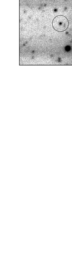
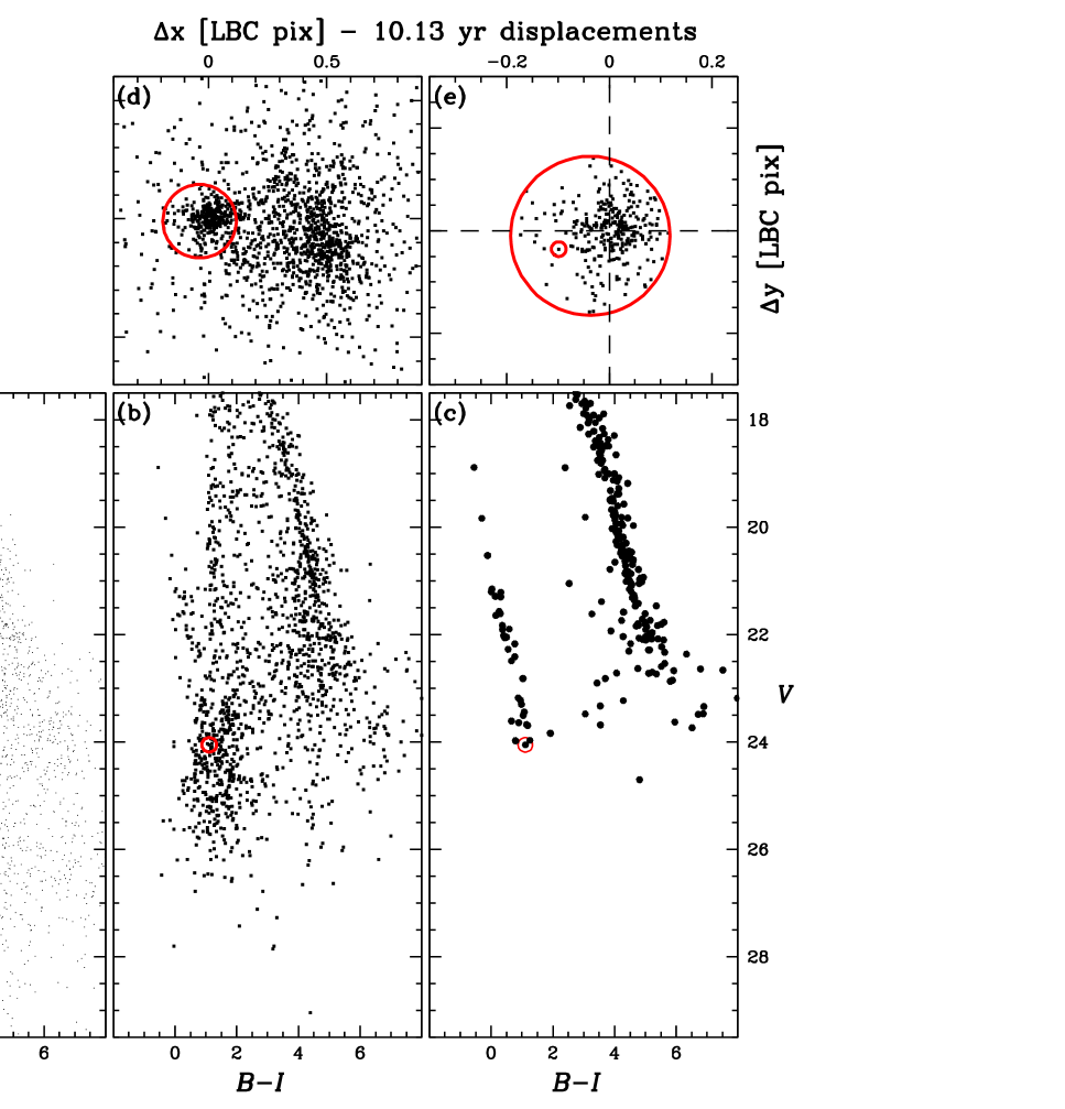
Figure 4: Panel (a) shows the $V$ vs. $B-I$ CMD for all the objects in the target list. With our photometric-reduction technique we are able to measure sources as faint as $V$$\gtrsim$28. It is clear from the figure that the bulk of faint blue compact galaxies occupy the same region as the WDs. Panel (b) shows the same CMD for objects for which we have a proper motion measurement. Our proper motions can reach a magnitude of $V$$\sim$26. The relative VPD is shown in panel (d); a red circle includes the objects that we assumed to be cluster members (see text for details). Panel (c) shows the CMD for the cluster members only, as selected in panel (d). Panel (e) shows the zoomed VPD for members. A small red circle in panels (b), (c), (e) identifies the faintest WD. In order to show the significance of the detection of this WD, top-left panel shows a 40$\arcsec$$\times$40$\arcsec$ region of the $B$-stacked image around this star, that stands clearly above the background. The brightest pixel of this star has $\sim$75 DNs (sky subtracted) above a local sky noise of $\sim$4 DNs, therefore its detection is unambiguous.

3.4 Proper motions

Proper motions were obtained as described in Anderson et al. (anderson06 (2006)). Of the initial target list obtained from the peak map, we selected only those sources with a measure in both LBC $V$ and $B$ filters. This list is then used to calculate displacements between the two epochs, as follows.

We measured a chip-based flux and GD-corrected position using PSF-fitting for each object in the list in each chip of each exposure where it could be found. Then we organized the images in pairs of images from each epoch. For each object, in each pair, we computed the displacement (in the reference frame) between where the first-epoch predicts the object to be located, after having transformed its coordinates on the reference-frame system, and its actual-observed position in the second epoch image. Multiple measurements of displacements for the same object are then used to compute average displacements and rms.

It is clear that, in order to make these displacement predictions, we need a set of objects to be used as a reference to compute positional transformations between the two epochs for each source. The cluster members of M 67 are a natural choice, as their internal motion is within our measurement errors ($\sim$0.2 mas yr^-1 Girard et al. girard89 (1989)), providing an almost rigid reference system with the common systemic motion of the cluster.

We initially identified cluster members according to their location in the LBC $V$ vs. $B-V$ color-magnitude diagram. By predominantly using cluster members, we ensure proper motions to be measured relative to the bulk motion of the cluster. We iteratively removed from the member list those objects with a field-type motion even though their colors may have placed them near the cluster sequences. In our proper-motion selections (see panel (d) of Fig. 4), we considered as cluster members all sources whose displacement is within a circle of radius 0.15 LBC pixels in 10.13 yr [we found this to be the best compromise between losing (poorly measured) M 67 members and including field objects] in the vector-point diagram (VPD), slightly off-center with respect to the zero of the motion, in order to further reduce the number of field objects in our member list.

In order to minimize the influence of any uncorrected GD residual, proper motions for each object were computed using a local sample of members; specifically the 25 (at least) closest ($r$$<$3^′), well-measured cluster stars (see Anderson et al. anderson06 (2006) for more details). Note that, in order to maximize the cluster-field separation, we used all the available images, in every filter, in both epochs. Indeed, our aim here is to provide a pure sample of M 67 WDs, and we are not interested in removing systematic errors below the mas level at the expenses of the size of the WD sample. For a more careful proper motion analysis we refer the reader to the companion paper Bellini et al. (submitted).

Finally, we corrected our displacements for atmospheric differential chromatic refractions (DCR) effects, as done in Anderson et al. (anderson06 (2006)). The DCR effect causes a shift in the photocenter of sources, which is proportional to their wavelength, and a function of the zenithal distance: blue photons will occupy a position that differs from that of red photons. Unfortunately, within each epoch, the available data sets are not optimized to perform the DCR correction directly. We can, however, check if possible differences in the DCR effects between the two epochs could generate an apparent proper motion for blue stars relative to red stars.

We selected two samples of cluster member stars, one made by WDs in the magnitude interval 20$<$$V$$<$23, and the other on the MS, within the same magnitude interval. For each sample, we derived the median $B-V$ color and the median proper motion along the $X$ and $Y$ axes, with dispersion obtained as the 68.27^th percentile around the median. We used a linear fit to derive the DCR corrections along both axes, as done in Anderson at al. (anderson06 (2006)). We found that DCR corrections were always below 0.7 mas yr^-1 $(B-V)^{-1}$.

In panel (b) of Fig. 4 we show the $V$ vs. $B-I$ CMD of all the sources for which we have at least two individual displacement measurements. The red circle in the figure marks the location of the faintest M 67 WD measured in this work. It is clear from panel (b) that we can measure proper motions of sources more than two magnitudes fainter than this star. Panel (d) in the same figure shows the VPD of the sources in panel (b). Since we used M 67 star members as reference to compute displacements between the two epochs, the origin of the coordinate coincides with the M 67 mean motion. The red circle in panel (d) show our adopted membership criterion.

The cluster-field separation is $\sim$0.5 pixel in 10.13 yr ($\sim$11 mas yr^-1). This separation is consistent with the one presented in Yadav et al. (yadav08 (2008)). A detailed comparison, and the merged catalogs, will be given in a companion paper and will deliver to the community the —so far— most complete catalog of M 67 members.

The $V$ vs. $B-I$ CMD of the selected cluster members is shown in panel (c), and the corresponding VPD is shown (enlarged for a better reading) in panel (e). Again, we highlighted the position of the faintest measured M 67 WD with a small circle, in both panels. It is clear from panel (c) that the WD CS sharply drops at $V$$\sim$24.1. This magnitude marks the bottom of the WD CS of M 67. The faintest WD has a proper motion consistent with the M 67 mean motion [see panel (e)]. A visual inspection of all the M 67 WDs on our stacked images confirmed that all of them are real stars.

3.5 Completeness

A complete investigation of the WD CS would require also the study of the WD LF. However, a proper study of the LF requires an appropriate estimate of the completeness of the star counts.

Computing completeness corrections taking into account both photometry and proper motions is a very complex and delicate matter, which is beyond the capability of our software, which was developed with the specific aim of deriving the most precise photometry and proper motions. A completeness correction that takes carefully into account proper motions opens a new series of problems, has never been properly treated in the literature. The aim of the present paper is to extract a clean sample of M 67 WD members to precisely locate them on the CMD, to study their main properties and to constrain theory. Our catalog will provide observers with a set of bona-fine WDs for spectroscopic follow-up investigations (at least for the bright WDs). We located the bottom of the WD CS just where the CS ends, not using statistical subtractions in the LF, as done, e.g. by R98 on the same cluster. However, it is important to emphasize here that our photometry and astrometry extends far below (about two magnitudes at the color of the faintest WD) the sharp WD CS cut off. Moreover, as shown by R98, at the $V$$<$25, the completeness, even in the shallower CFHT images, is $>$95%. We do not expect that our reduction software and the proper motion selection procedure can lower this completeness in any significant way. We defer the analysis of the completeness to when a new set of LBC images (project already approved by LBT TAC) will be available, providing a third epoch for a much more accurate proper motion measurement.

4 Comparison with previous studies

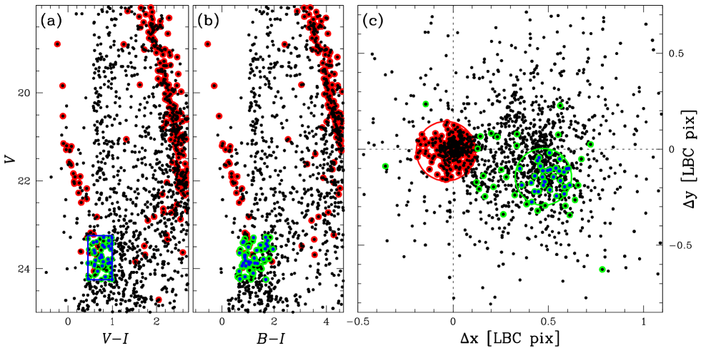
Figure 5: (a) $V$ vs. $V-I$ CMD zoomed around the end of WD CS of M 67. (b): $V$ vs. $B-I$ CMD of the same region. In both panels, black dots are objects with proper motion measurements. Red circles mark probable M 67 members, as defined in Section 3.4. In (a) we selected a sample of objects (highlighted with a blue rectangle), superimposed onto the end of the WD CS, which lie in the region of the CMD used by R98 to define the last two bins of his LF. (c): show the VPD of all the sources. In red are M 67 members (within the red circle), and in green color are the object within the rectangle in panel (a). In blue (in all the three panels) are those selected objects which proper motion is within 1 $\sigma$ [green circle in panel (c)] around their 3$\sigma$-clipped median motion.

A thorough study of the WD CS in M 67 was already presented by R98. In R98, the authors removed background galaxies by mean of stellar-like shape parameter selections, and by statistically subtracting objects as measured in a blank field $\sim$$1\aas@@fstack{\circ}2$ away from the center of M 67. As we can see in our stacked images, the majority of faint objects are indeed blue compact galaxies, stockpiled at the same location in the CMD as the end of the WD CS (see Fig. 4). We can also see that the faint galaxies are almost unresolved. This means that their profiles could mimic stellar profile, making the shape-like parameter selection criteria not very efficient. Moreover, a statistical subtraction of these galaxies using a blank field is subject to the problem of the cosmic variance (presence of cosmological structures that alter the statistics of extra-galactic background objects in different directions, within limited FoVs).

After the shape selection, R98 extracted the stars for the WD LF around a 0.7 $M_{\odot}$ CS derived using the interior models of Wood (wood95 (1995)) and the atmospheres of Bergeron, Wesemael, and Beauchamp (bwb95 (1995)). In summary, in R98 WD are never identified. Their LF has been derived only defining a strip on the CMD for object selection, and then applying a statistical subtraction of field objects. Despite all the aforementioned difficulties, the LF derived in R98 clearly shows a pile-up around $V$$\simeq$24 [and $(V-I)_{0}$$=$0.7], and it terminates at $V$$\simeq$24.25. These values are in very good agreement with the WD CS termination of $V$=24.1$\pm$0.1 that we find with our proper-motion selected sample of WDs.

The sharp peak of the LF identified with the bottom of the WD CS by R98 needs some more investigation. We can note, in our $V$ vs. $B-I$ CMD [panel (b) of Fig. 4], a clump of objects very close to the end of the WD CS, but slightly redder. The same objects are almost superimposed onto the WD CS if we look at the $V$ vs. $V-I$ CMD used by R98 in their investigation. The average $V-I$ color of these objects is $\sim$0.8, close to the $(V-I)_{0}$$\simeq$0.7, where R98 found a pile-up of objects that were treated by R98 as the bottom of the WD CS (note that R98 use 0.5 magnitude wide bins in color to select their WD candidates). We now further investigate the nature of these objects.

In Fig. 5 we plot our $V$ vs. $V-I$ and $V$ vs. $B-I$ CMDs in panels (a) and (b), respectively. Black dots are objects for which we have a proper motion measurement. Probable M 67 members, as defined in Section 3.4, are highlighted in red in both panels. In panel (a) we selected for investigation those objects within a (blue) rectangle, whose borders are defined as $V-I$$=$0.7$\pm$0.25, $V$=24.25, and $V$=23.25. This region of the $V$ vs. $V-I$ CMD is the same one used by R98 to define the last two bins of their WD LF. Panel (c) displays the VPD of the sources plotted in panels (a) and (b), on which we have marked in red our proposed M 67 members (stars within the red circle defined in Section 3.4), and in green the objects within the rectangle. Very few of these objects have a displacement that is close to the mean M 67 motion, and therefore could be M 67 stars, but the majority of them is concentrated around a location in the VPD that is close to the centroid of the motion of galaxies (Bellini et al. submitted). Therefore, by means of proper motion measurements, we conclude that the vast majority of the objects that form the clump close to the end of the WD CS are field-type objects, and not M 67 members.

As a further proof that these objects are mainly background galaxies, we performed the following test. We calculated the 3$\sigma$-clipped median displacement (where $\sigma$ is the rms of the residuals around the median) of these objects on the VPD, and selected the ones within 1 $\sigma$ from this position [big green circle in panel (c)]. This subsample, constituted by 31 objects, is highlighted in blue in all the three panels. We used the LBC $V$ image of 330 s exposure (the deepest we have, and one with the best seeing $\sim$$0\aas@@fstack{\prime\prime}7$) to check whether or not these objects are actually galaxies or stars. Only 21 of them are present in this image. We measured the full width at half maximum (FWHM) along both LBC $X$ and $Y$ axes. PSF shapes and orientation vary with location on the chip, and from chip to chip; moreover, also galaxy shapes and orientations do vary. Nevertheless, we expect that, on average, the measured FWHMs of galaxies to be larger than the ones of stars.

In order to measure FWHMs of stars for this comparison, we selected 10 M 67 WDs in the same $V$ magnitude interval as the investigated objects. Five of them are present in the 330 s image. We measured the FWHM for these 5 stars, again along both LBC $X$ and $Y$ axes. We then measured average values and errors for the FWHMs of stars and suspected galaxies. The results are as follows:

$${\rm stars:\leavevmode\nobreak\ \leavevmode\nobreak\ }\left\{\begin{array}[]{l}\overline{\rm FWHM}^{\ast}_{X}=3.2\pm 0.1\\ \overline{\rm FWHM}^{\ast}_{Y}=2.9\pm 0.2\\ \end{array}\right.$$

$${\rm objects:\leavevmode\nobreak\ \leavevmode\nobreak\ }\left\{\begin{array}[]{l}\overline{\rm FWHM}^{\rm obj.}_{X}=4.0\pm 0.1\\ \overline{\rm FWHM}^{\rm obj.}_{Y}=3.7\pm 0.1\\ \end{array}\right.$$

It is clear that objects within the green circle in panel (c), are sizably broader than WDs at the same luminosity, by $\sim$25% in both $X$ and $Y$ axes. On the basis of their average shape and of their proper motions, we conclude that the objects are indeed blue faint galaxies and not M 67 stars. This result does not invalidate what was done in R98, since we already showed that our estimated WD CS end, based on a pure sample of M 67 members, is in very good agreement with the R98 determination. However, we caution the readers to use the WD LF to infer information on the M 67 WD properties before an accurate LF, corrected for completeness, and based on a field-object cleaned WD CS can be produced.

5 Comparison with theory

In the same vein as our previous papers on the WD populations in Galactic star clusters (see, e.g. Bedin et al. bedin09 (2009) and references therein), we compare the M 67 WD CS with theoretical WD models, and also assess the consistency with the results from modeling of the cluster’s MS and turn off (TO) regions.

As a first step of our analysis, we compare the BaSTI [Fe/H]=+0.06 scaled solar isochrones (Pietrinferni et al. pietr04 (2004)) for an age of 3.75 and 4.00 Gyr to the (single stars only) $V$ vs. $V-I$ CMD by Sandquist (sand04 (2004)) that covers MS, TO, red-giant branch (RGB) and the central He-burning phases. As shown in Fig. 6, the best fit to the MS and post-MS phases implies $(m-M)_{0}$=9.64 and E($B-V$)=0.023 [obtained from the E($V-I$) by using the Cardelli et al. (cardelli89 (1989)) extinction law, with $R_{V}$=3.1]. These values are consistent —within the uncertainties— with the recent [Fe/H]=$+$0.05$\pm$0.02 and E($B-V$)=0.04$\pm$0.03 derived by Pancino et al. (pancino09 (2009)), and with the $(m-M)_{0}$=9.60$\pm$0.09 obtained by Percival & Salaris (percival03 (2003)). We will also adopt these values in the following, for comparisons of the observed WD sequence with theory.

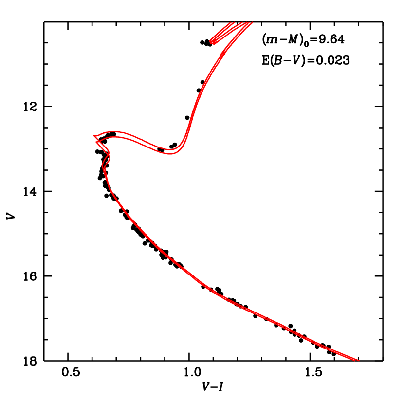
Figure 6: Fit of $V$ vs. $(V-I)$ CMD by Sandquist (sand04 (2004)) with the BaSTI 3.75 and 4 Gyr isochrones with [Fe/H]=+0.06 and convective core overshooting.

Had we used a lower [Fe/H] in the fit to the Sandquist data set, the match to the RGB and red clump would have improved, but at the expense of the fit to the MS (the slope would not be matched as well as before). Had we lowered the [Fe/H] value in our isochrones by 0.1 dex (more than three times the quoted error bars from the spectroscopic determinations in Pancino et al. pancino09 (2009)) the resulting distance modulus from the overall fit would have increased by only a few (2–3) hundredths of a magnitude, the reddening by $\lesssim$0.01 mag, and the age would have hardly changed. All in all, the overall picture regarding distance, reddening and age would not be changed appreciably. This works in our favor, because these quantities are what matters most for the comparison with the WD CS. Moreover, the termination of the theoretical WD isochrones would not be really affected, because the luminosity of the faintest WDs is essentially driven by their cooling timescales, rather than the progenitor lifetimes (higher mass progenitors with small life times compared to the age of the cluster).

Fig. 6 shows that the best TO age estimate is 3.8–4.0 Gyr for BaSTI isochrones with convective core overshooting, in agreement with previous results (Carraro et al. carraro96 (1996) and R98). A problem (Carraro et al. carraro96 (1996)) persists with the cluster RGB, which is significantly bluer for the same set of parameters, independently from the adopted models. We note that, at the age of M 67, the mass extension of convective cores in TO stars is small, and the overshooting extension in the BaSTI models (and in general in all models including convective core overshooting) is in the regime of shrinking to zero with decreasing convective core masses (see Pietrinferni et al. pietr04 (2004) for details).

The observed WD sequence is compared to a reference set of H-atmosphere (DA) CO-core WD isochrones computed using the Salaris et al. (salaris00 (2000)) WD tracks, bolometric corrections from Bergeron, Wesemael, & Beauchamp (bwb95 (1995)), progenitor lifetimes from the BaSTI (Pietrinferni et al. pietr04 (2004)) scaled solar models with [Fe/H]=+0.06 (the same used in the fit to the MS and TO regions), and the initial-final mass relationship (IFMR) from Salaris et al. (salaris09 (2009)) extrapolated at its lower end to the TO mass of M 67. We have also employed, as a test, the relationship proposed by Kalirai et al. (kalirai09 (2009)) and found negligible differences in the resulting isochrones.

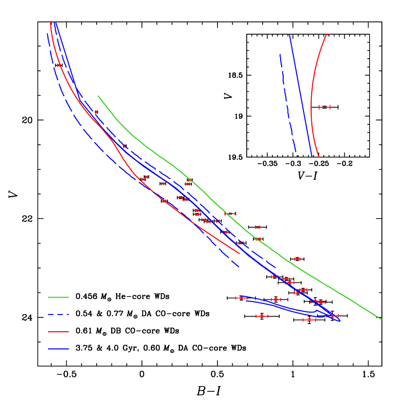
Figure 7: $V$ vs. $(B-I)$ CMD of the WD sequence compared to our reference CO-core DA WD isochrones with age of 3.75 and 4 Gyr (blue solid lines), CO-core DA cooling tracks with masses equal to 0.54 $M_{\odot}$ and 0.77 $M_{\odot}$ (dashed blue lines), a 0.465 $M_{\odot}$ He-core WD (green solid line) and CO-core 0.61 $M_{\odot}$ DB track (red solid line). All isochrones and tracks have been shifted by the reference distance modulus and reddening values used in Fig. 6. The inset shows the position in the $V$ vs. $V-I$ CMD of the brightest WD in our data compared to the reference isochrones, the 0.77 $M_{\odot}$ DA track and the DB track. Red error bars are our formal errors, black error bars are external estimates of the errors. See text for details.

Figure 7 displays our WD isochrones for 3.75 and 4 Gyr, again using with $(m-M)_{0}$=9.64 and E($B-V$)=0.023 as in Fig. 6, compared to the observed WD cooling sequence in the $V$ vs. $B-I$ CMD. The choice of this wide-color baseline enhances differences in the location of WDs due to variation in their mass or atmosphere composition, compared to either $B-V$ or $V-I$ —the other colors available from our photometry—, and provides more stringent tests for the theoretical modeling of the observed sequence. [In addition, $V$ and $B-I$ photometric errors are independent.] Red error bars in Fig. 7 are the formal photometric errors directly derived from the uncertainty in the fit slope in Equation 2 (i.e., the internal errors).

Formal errors are generally a lower bound for the true errors. To obtain a more reliable —external— estimate of the errors, we randomly divided our photometric data set (for each filter) into four subsamples. Specifically, each of the four LBC $B$ subsamples is constituted by 14 images, each LBC $V$ subsample by 11 images, while UH8K $I$ images are splitted into 3 groups of 3 images each, and a last group made with 2 images only (for a total of 11 images).

We selected only the WDs in our sample (see Fig. 7), and for each subsample separately, we repeated the last reduction step of our three-step procedures (see Section 3.3) to compute their $BVI$ fluxes. For each WD, we obtained four independent measurements of the flux (in each filter), with formal errors. We weighted the four estimates of these fluxes according the their formal errors, and took a weighted mean of the four fluxes. We found that this mean flux was equal, within the round-off errors, to the value that we had found using the whole data set. [It was within few percent in nearly every case.] Finally, we derived an external estimate of the true photometric error, from the residuals of the individual values of the flux from their mean, using the same weights as we had used for the mean. These external photometric errors are indicated by the black error bars in Figure 7.

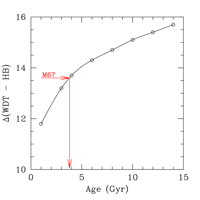
Figure 8: The theoretical value $\Delta V({\rm WDT-HB})$ is plotted against the age of the simulated cluster. The value observed for M 67 in the present work is also shown.

We note, instead, that error estimates based on artificial stars are also (as our formal internal errors) generally underestimated, and so less reliable. This is because artificial stars are always based on an input PSF model, which could significantly differ from the true local PSF, concealing our ignorance about the true sources’ flux. Moreover, thanks to the large dither pattern of LBC observations, WDs fall each time in different locations on the LBC chips, in different chips as well, and under different observing conditions, contributing to further strengthening the reliability of the external estimates of the errors.

There is good agreement between the location of the WD isochrones and the observed sequence. The expected blue hook at the bottom of the WD sequence is also visible in the data. It is due to the presence of increasingly massive (lower radius) objects originating from more massive MS progenitors that had more time to cool down along the WD sequence. The location and color extension of the blue hook is well matched by the isochrones with ages consistent with the TO age. We recall that the observed $V$ magnitude of the bottom end of the WD sequence ($V$$\sim$ 24.1$\pm$0.1 mag) is in very good agreement with the observed WD LF by R98, and with the predictions by Brocato, Castellani & Romaniello (bcr99 (1999), their Fig. 8), where an age of 4 Gyr, solar metallicity and a distance modulus $(m-M)_{0}$=9.6 were assumed.

A complementary method to estimate the age of M 67 uses a new age indicator, that has the advantage of being free from distance and extinction effects, and it is also independent from the age obtained from the TO. Similarly to the $\Delta V$ parameter employed in globular cluster studies ($V$-magnitude difference between the Horizontal Branch and Turn Off, see e.g., the review by Stetson, Vandenberg & Bolte stetson96 (1996)) it is possible to define the parameter $\Delta V({\rm WDT-HB})$ as the difference between the $V$ magnitude of the WD CS end [$V$(WDT)], and the mean level of the horizontal branch [$V$(HB) —see Brocato, Castellani & Romaniello bcr99 (1999)]. Once the metallicity of the cluster is known, this parameter is a function of the cluster age, increasing for older clusters (see Fig. 8). Here, we present the calibration of $\Delta V({\rm WDT-HB})$ as a function of age for M 67 metallicity, while the general calibration for a wider range of chemical compositions will be presented in a forthcoming paper (Brocato et al.  in prep.). Here it suffices to say that our data provide $\Delta V({\rm WDT-HB})$=13.6$\pm$0.1, that leads to an age of 3.9$\pm$0.1 Gyr. This estimate (which is formally independent of the CMD fitting procedure used in Fig. 6 to estimate the cluster age) is in agreement with the other estimates above discussed.

6 Discussion

Despite the good agreement between the location of the WD isochrone and the observed CS, and the consistency between TO and WD ages, in the $V$ magnitude interval between $\sim$19 and $\sim$23 there are several objects that appear more than 3$\sigma$ away from the theoretical sequence, and deserve a further analysis. We cannot exclude, a-priori, that these objects are WD+WD binaries, but this possibility is very unlikely, therefore in the following we will not treat this case. We have first considered the possible presence of a large spread in the cluster IFMR (see, e.g., Salaris et al. salaris09 (2009) and Dobbie et al. dobbie09 (2009)) for progenitor masses in the range $\sim$1.5–2.5 $M_{\odot}$. Figure 7 shows the cooling tracks of 0.54 $M_{\odot}$ and 0.77 $M_{\odot}$ DA CO-core WDs (dashed blue lines). In the appropriate magnitude range these two models are located on the red and blue side of the reference isochrone, respectively, that is populated by WDs with mass $\sim$0.6 $M_{\odot}$. A spread of the IFMR towards higher values of WD masses can be explained by the spread of objects on the blue side of the isochrone, whereas the redder WDs are not so easy to explain. The 0.54 $M_{\odot}$ track is still about 0.1 mag bluer than 6 objects with $V$ between $\sim$19 and $\sim$23. Taking into account that the core mass at the first thermal pulse is $\sim$0.52–0.53 $M_{\odot}$ for the relevant progenitor mass range, it is difficult to match the position of these red objects with “standard” WD sequences. A possible way out of this problem is to invoke the presence of CO-core WDs with masses lower than the core masses at the beginning of the thermal pulse phase. As studied by Prada Moroni & Straniero (prada09 (2009)), anomalous and somewhat finely tuned mass loss processes during the RGB phase can produce CO-core WDs with masses as small as $\sim$0.35 $M_{\odot}$ at the metallicity of M 67, for progenitors around 2–2.3 $M_{\odot}$. In this mass range there is a transition between electron degenerate and non degenerate He-cores along the RGB. These low mass WDs are potentially able to match the handful of objects redder than our reference isochrone. Their cooling timescales (e.g. Fig. 12 in Prada Moroni & Straniero prada09 (2009)) are roughly consistent with their observed luminosities, assuming that they are produced by progenitors with masses around 2–2.3 $M_{\odot}$.

There is another possible interpretation. In order to reproduce the position of these WDs in the CMD, we have considered the cooling track (green line in Fig. 7) of the 0.465 $M_{\odot}$ He-core WD discussed in Bedin et al. (2008a ). At the cluster’s metallicity, BaSTI models predict that the He-core mass of stars climbing the RGB (mass $\sim$1.4 $M_{\odot}$) can be at most equal to $\sim$0.47 $M_{\odot}$. This WD track represents therefore an approximate bluer boundary for the location of M 67 He-core WDs. All of the 6 red objects (that are more than 3$\sigma$ away from the CO-core WD isochrone) lie close to this sequence. They can be massive He-core WDs produced by very efficient mass loss along the RGB phase. These same 6 objects are located around the He-core sequence also in $V-I$ colors although the separation between the sequences is smaller in that case (and even smaller in $B-V$). As for the objects at the blue side of the isochrones, Fig. 7 displays the cooling track of a 0.61 $M_{\odot}$ CO-core model with pure He-atmospheres (DB, red solid line). This is approximately the expected value of the DB mass evolving down to $V$$\sim$23 (where the track is truncated) for the chosen progenitor lifetimes and IFMR. At fainter magnitudes, DA and DB tracks of the same mass have approximately the same colors.

There is clearly one object at $V$$\sim$19, and two objects with $V$ between $\sim$21 and 22, that are well matched by the DB model and are therefore candidates to be He-atmosphere WDs. It is clear that without spectroscopic estimates of atmospheric composition and/or WD masses it is impossible to find a unique interpretation for these WDs that are not matched by the reference isochrone. But both $B-I$ and $V-I$ colors suggest that the brightest object at $V$$\sim$19 is a DB WD. The inset of Fig. 7 displays the position of this star in the $V$ vs. $V-I$ CMD. In this CMD the bright part of the DB sequence is located on the red side of the reference DA isochrone, whereas at magnitudes fainter than $V$$\sim$20 the relative position of the two sequences is the same as in the $B-I$. The star is located at the red side of the DA isochrone in $V-I$, and at the blue side of the isochrone in the $B-I$, exactly as expected for DB objects, and in complete disagreement with its interpretation as a massive DA object.

- (1) Anderson, J., Bedin, L. R., Piotto, G., Yadav, R. S., & Bellini, A. 2006, A&A, 454, 1029
- (2) Anderson, J. et al. 2008, AJ, 135, 2055
- (3) Bedin, L. R., Salaris, M., Piotto, G., King, I. R., Anderson, J., Cassisi, S., & Momany, Y. 2005, ApJ, 624, L45
- (4) Bedin, L. R., King, I. R., Anderson, J., Piotto, G., Salaris, M., Cassisi, S., & Serenelli, A. 2008, ApJ, 678, 1279 (2008a)
- (5) Bedin, L. R., Salaris, M., Piotto, G., Cassisi, S., Milone, A. P., Anderson, J., & King, I. R. 2008, ApJ, 679, L29 (2008b)
- (6) Bedin, L. R., Salaris, M., Piotto, G., Anderson, J., King, I. R., & Cassisi, S. 2009, ApJ, 697, 965
- (7) Bellini, A., et al. 2009, A&A, 493, 959
- (8) Bellini, A., & Bedin, L. R. 2009, PASP, 121, 1419
- (9) Bellini, A., & Bedin, L. R., submitted
- (10) Bellini, A., et al., submitted
- (11) Bergeron, P., Wesemael, F., & Beauchamp, A. 1995, PASP, 107, 1047
- (12) Brocato, E., Castellani, V., & Romaniello, M. 1999, A&A, 345, 499
- (13) Cardelli, J. A., Clayton, G. C., & Mathis, J. S. 1989, ApJ, 345, 245
- (14) Carraro, G., Girardi, L., Bressan, A., & Chiosi, C. 1996, A&A, 305, 849
- (15) Dobbie, P. D., Napiwotzki, R., Burleigh, M. R., Williams, K. A., Sharp, R., Barstow, M. A., Casewell, S. L., & Hubeny, I. 2009, MNRAS, 395, 2248
- (16) Fellhauer, M., Lin, D. N. C., Bolte, M., Aarseth, S. J., & Williams, K. A. 2003, ApJ, 595, L53
- (17) Giallongo, E., et al. 2008, A&A, 482, 349
- (18) Girard, T., Grundy, W., Lopez, C., & van Altena, W. 1989, AJ, 98, 227
- (19) Kalirai, J. S., Saul Davis, D., Richer, H. B., Bergeron, P., Catelan, M., Hansen, B. M. S., & Rich, R. M. 2009, ApJ, 705, 408
- (20) Pancino, E., Carrera, R., Rossetti, E., & Gallart, C. 2009, arXiv:0910.0723
- (21) Percival, S. M., & Salaris, M. 2003, MNRAS, 343, 539
- (22) Pietrinferni, A., Cassisi, S., Salaris, M., & Castelli, F. 2004, ApJ, 612, 168
- (23) Prada Moroni, P. G., & Straniero, O. 2009, A&A in press, arXiv:0909.2742
- (24) Richer, H. B., Fahlman, G. G., Rosvick, J., & Ibata, R. 1998, ApJ, 504, L91 (R98)
- (25) Salaris, M., García-Berro, E., Hernanz, M., Isern, J., & Saumon, D. 2000, ApJ, 544, 1036
- (26) Salaris, M., Serenelli, A., Weiss, A., & Miller Bertolami, M. 2009, ApJ, 692, 1013
- (27) Sandquist, E. L. 2004, MNRAS, 347, 101
- (28) Stetson, P. B., Vandenberg, D. A., & Bolte, M. 1996, PASP, 108, 560
- (29) Wood, M. A. 1995, White Dwarfs, 443, 41
- (30) Yadav, R. K. S., Bedin, L. R., Piotto, G., Anderson, J., Villanova, S., Platais, I., Pasquini, L., Momany, Y., & Sagar, R. 2008, A&A, 484, 609